


Multi-Objective Optimization of a Solar Combined Power Generation and Multi-Cooling System Using CO2 as a Refrigerant


Abstract
:1. Introduction
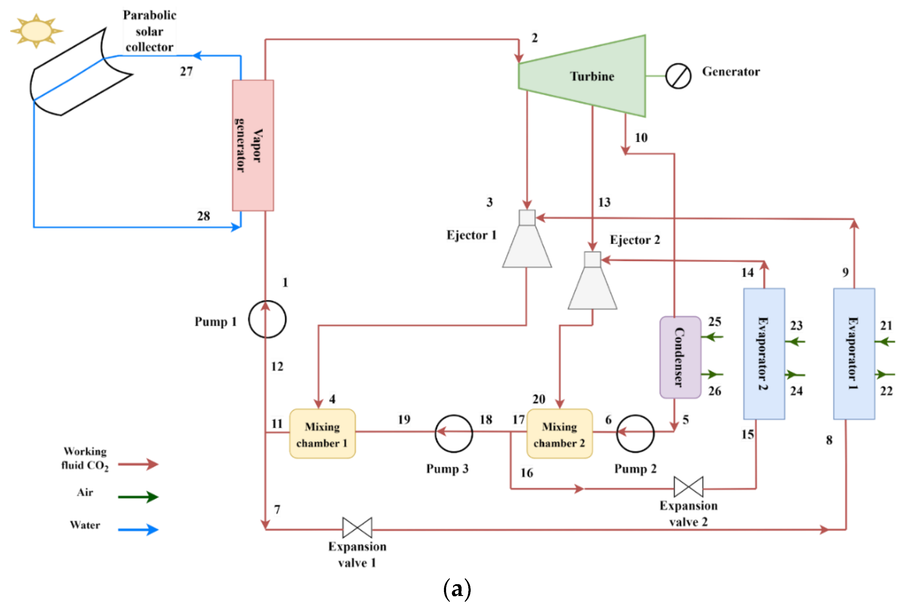
2. The System’s Description
3. The System’s Energetic Analysis
- Heat transfer between machinery, pipes, and the environment is disregarded, and the system is steady.
- Heat exchangers and pipe pressure drops are ignored.
- When the primary and secondary flows enter the ejector, they are both saturated vapor.
- There is no heat loss as the ejector operates in a constant condition.
- The isenthalpic evolution in the expansion valve.
- Constant isentropic efficiency for the turbine and pump are 90% and 80%, respectively.
- The ambient reference temperature and pressure are 25 °C and 1 atm, respectively.
- The steam generator efficiency is assumed to be 0.5.
- The entrainment ratio of ejector 1 and ejector 2 is assumed to be 0.3 and 0.45, respectively.
3.1. PTC Modeling
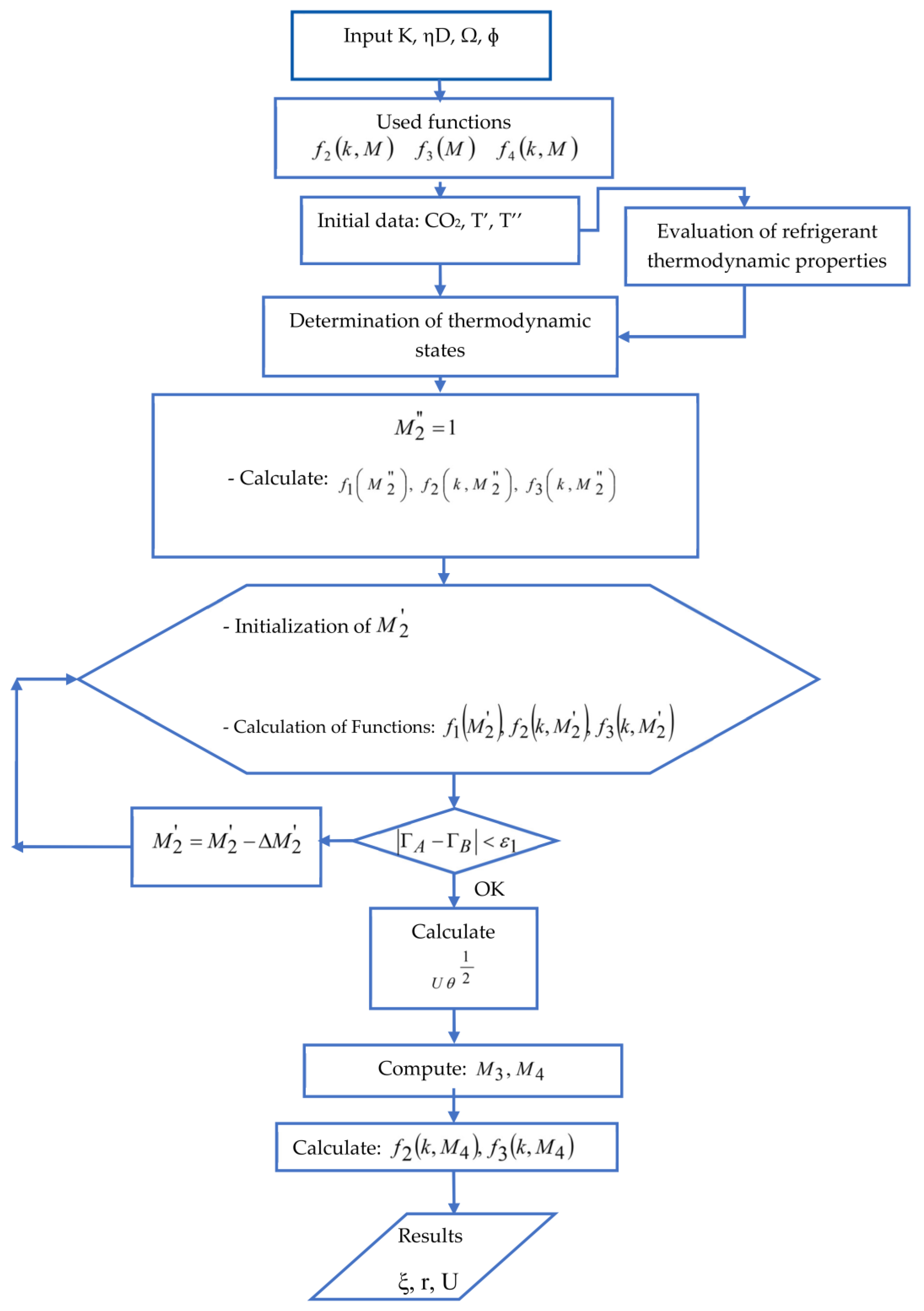
3.2. Ejector Modeling
- An ideal gas working fluid with constant thermal conductivity, k, and heat-specific heat capacity, Cp.
- Steady flow inside the ejector.
- Before mixing, the isentropic relations are utilized for simplicity in the 1D model.
- The two liquids are completely blended when they leave the mixing chamber.
4. The System’s Exergetic Analysis
5. The System’s Economic Analysis
6. The System’s Exergoeconomic Analysis
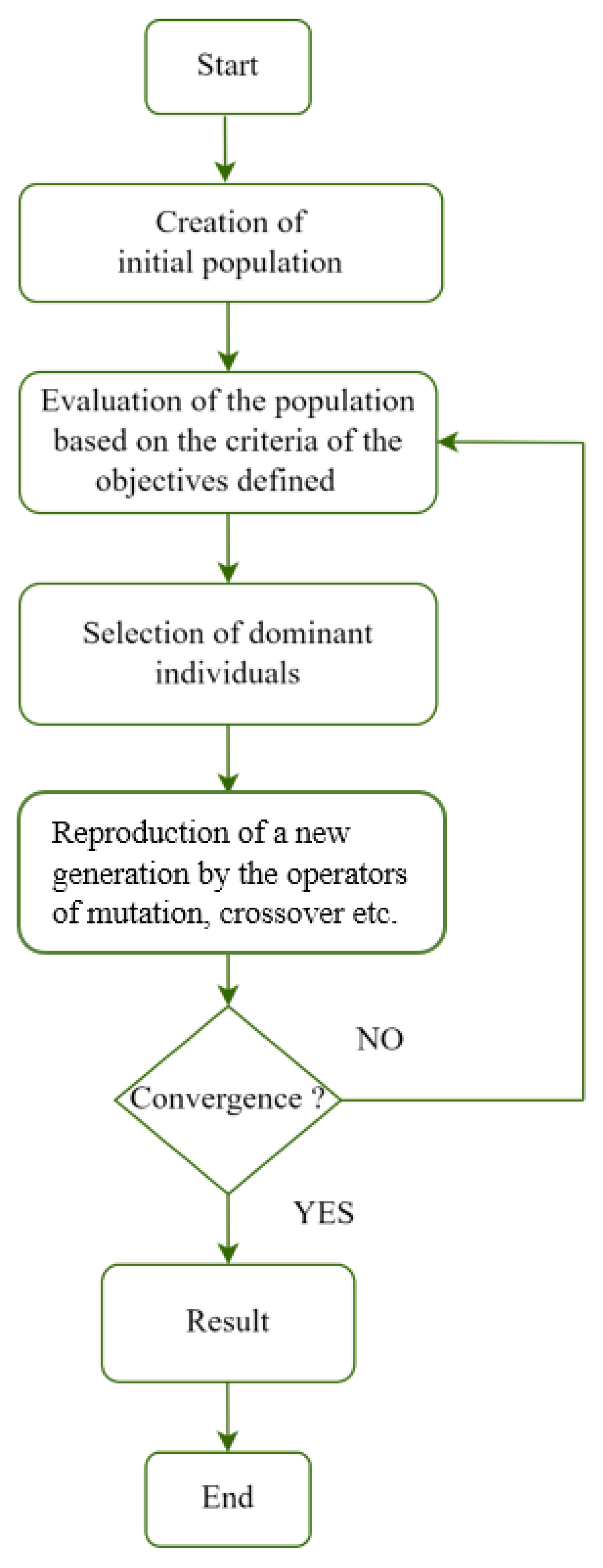
7. Multi-Objective Optimization
7.1. The Functions of Multi-Objective Optimization
7.2. The Decision Variables
8. Results and Discussion
8.1. Ejector Model Validation
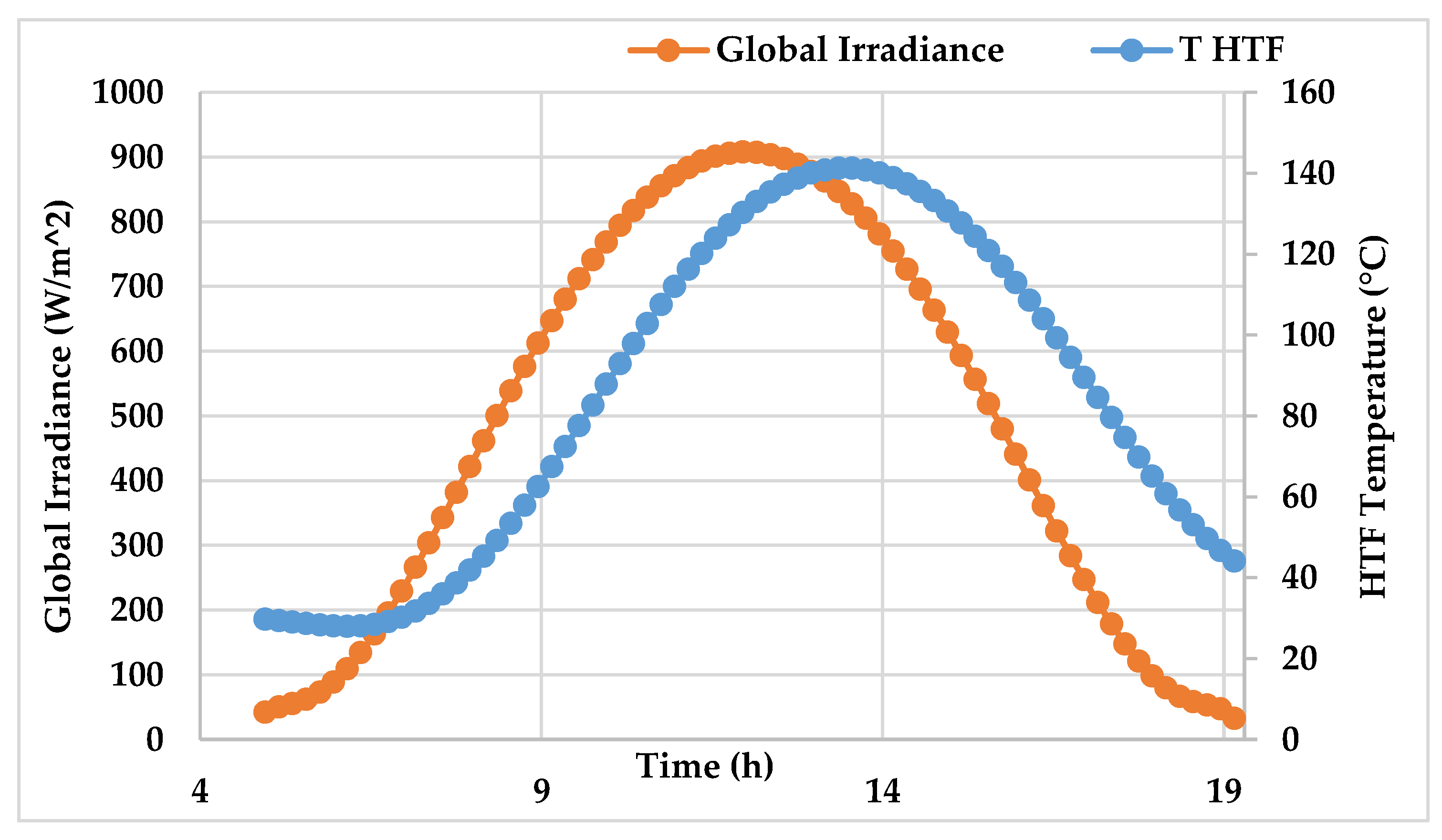
8.2. PTC Model Validation
8.3. Overall Results
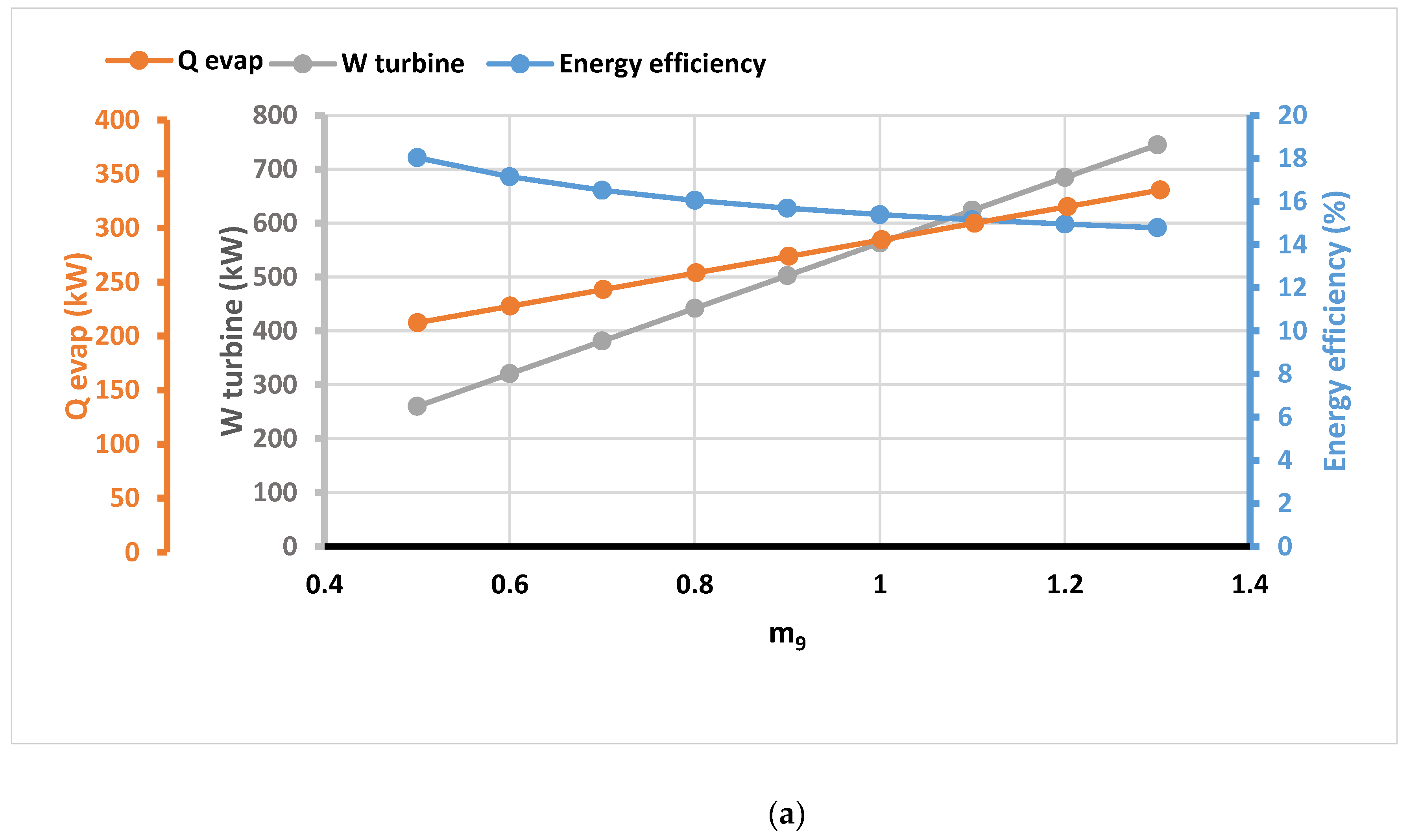
9. Parametric Study of Key Parameters
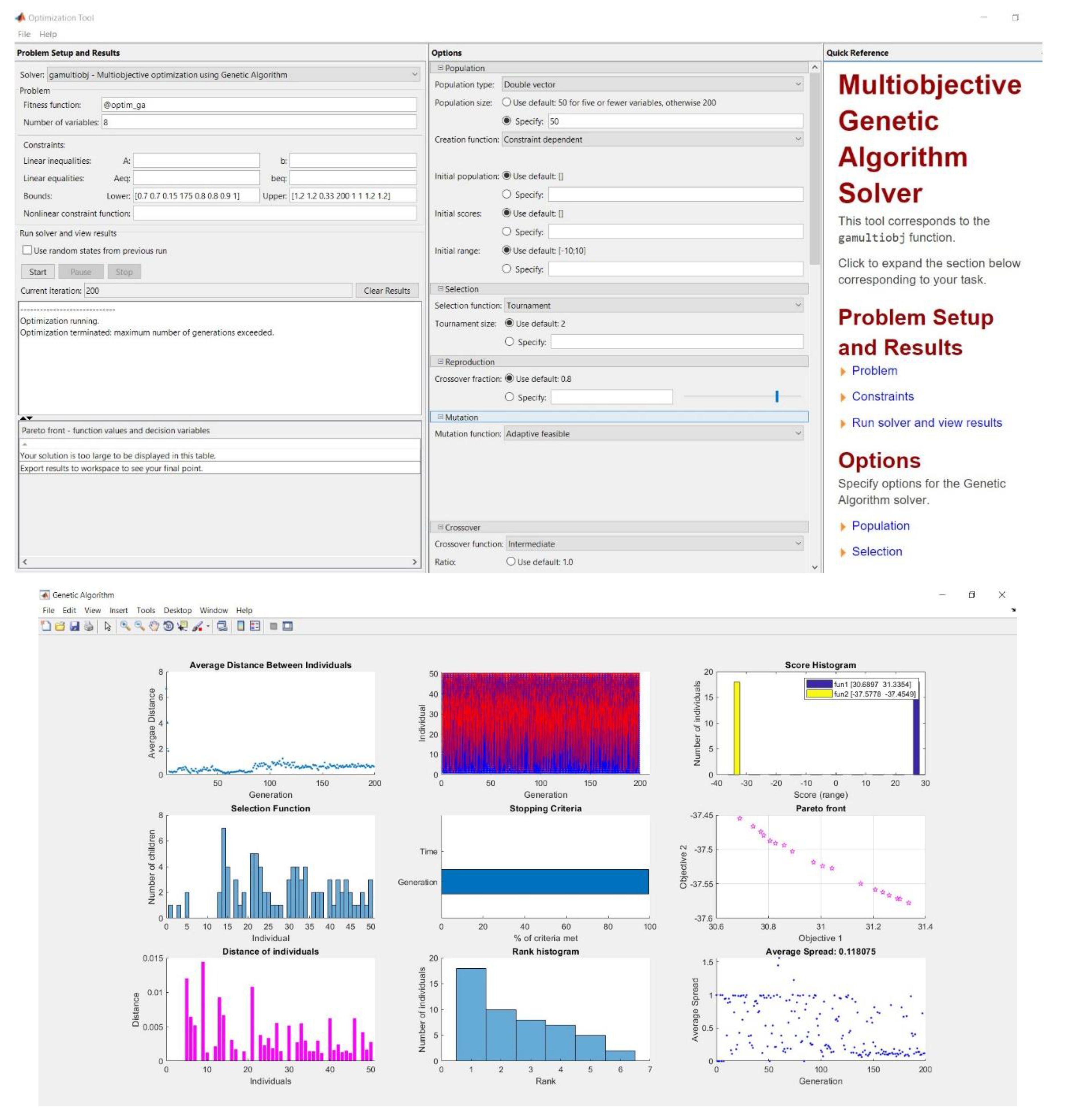
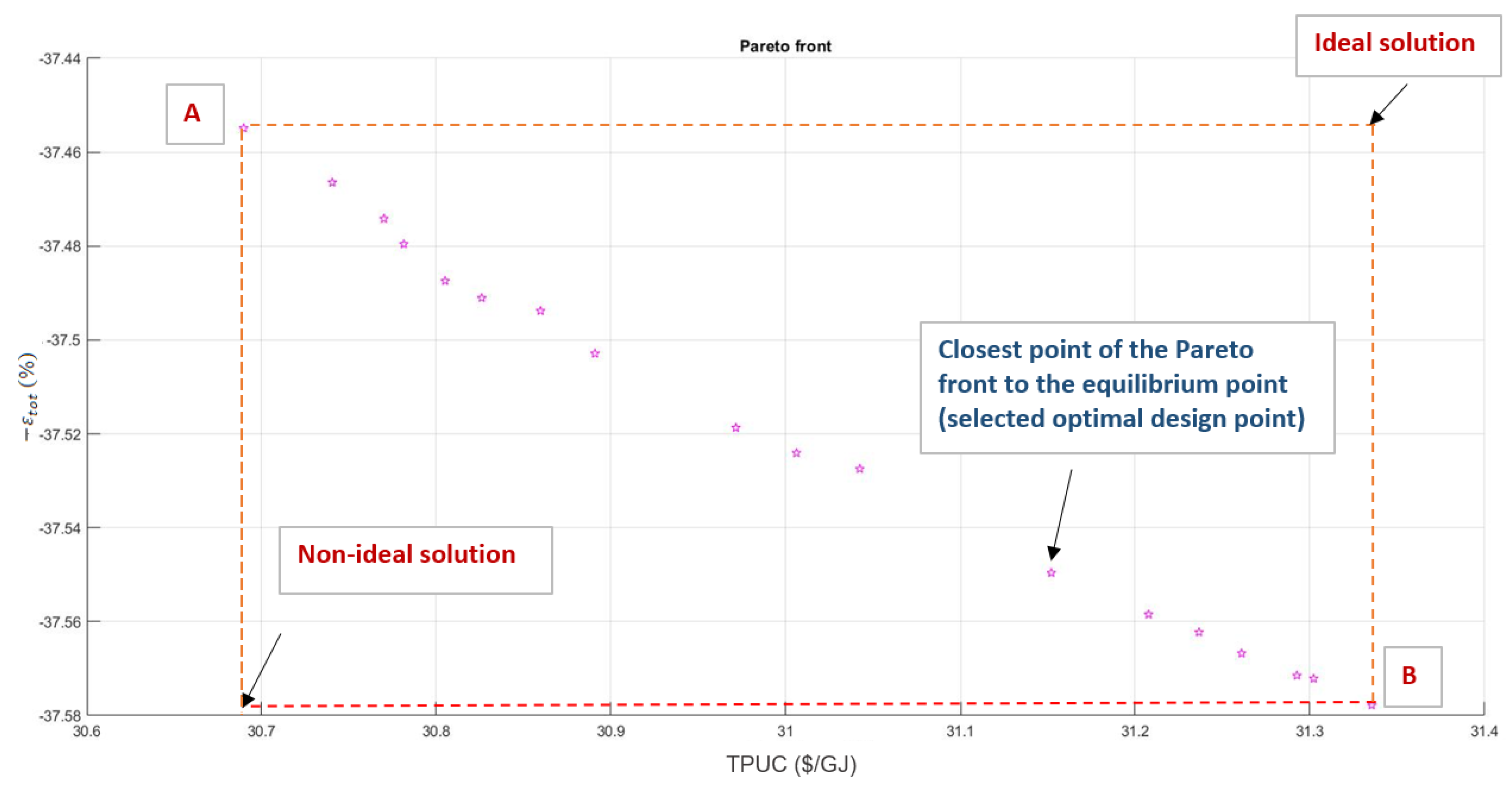
10. Optimization Results
- −
- Dispersions among individuals of the same generation.
- −
- Individual genealogy: the red, blue, and black lines represent the children of a mutation, a crossover, or elite, respectively.
- −
- A histogram of the values assigned by the objective functions for each generation,
- −
- The parents’ histogram, which contributed to the construction of succeeding generations.
- −
- The progression of the simulation’s stopping criterion.
- −
- The front or diagram of Pareto.
- −
- The dispersion between the individuals constituting the Pareto.
- −
- The rank of the individuals resulting from the simulation. The individuals of rank 1 constitute the Pareto front.
- −
- The average variations measured in the differences between individuals from one generation to the next.
11. Conclusions
Author Contributions
Funding
Data Availability Statement
Conflicts of Interest
Nomenclature
| Symbols | |
| A | Surface per unit length (m) |
| BB | Expansion ratio of the turbine |
| Cost rate (USD/h) | |
| C | Factor of concentration |
| Cp | Gas-specific heat at constant pressure, (kJ kg−1 K−1) |
| c | Specific exergy cost rate [USD/GJ] |
| Specific heat of the heat transfer fluid (kJ/kg K) | |
| D | Diameter (m) |
| d | Diverging outlet section diameter of the nozzle motor (m) |
| dD | Secondary nozzle diverging diameter (m) |
| d* | Nozzle motor diameter (m) |
| Exergy (kW) | |
| e | Specific exergy (kJ/kg) |
| FBM | Module factor |
| The exergoeconomic factor | |
| Gi | The solar global irradiance (kW/m2) |
| h | The enthalpy (kJ kg−1) |
| Convection heat transfer coefficient of the heat transfer fluid | |
| ieff | Rate of interest |
| k | Specific heat ratio (Cp/Cv) |
| IG | The solar direct radiation (kW/m2) |
| M | Mach number |
| Mass flow rate (kg s−1) | |
| n | Lifetime plant |
| P | Pressure |
| Q | Heat quantity (kJ) |
| Heat load (kW) | |
| S | The entropy (kJ/kg K) |
| r | The ejector compression ratio |
| The average inflation rate of the operating and maintenance cost | |
| The average inflation rate of the fuel cost | |
| The relative cost difference | |
| T | Temperature |
| t | Time (s) |
| U | The ejector entrainment ratio |
| Mechanical work (kW) | |
| Collector aperture (m) | |
| X | Driving nozzle position about the throat of the mixer (m) |
| Exergy destruction ratio | |
| Z | Distance (m) |
| The components’ cost rate [USD/h] | |
| Total system cost rate [USD/h] | |
| Abbreviations | |
| BMC | Bare module cost |
| CMCP | Combined multi-cooling and power generation |
| CEPCI | Chemical engineering plant cost index |
| CRF | Capital recovery factor |
| CELF | Constant escalation levelization factor |
| CC | Carrying charges |
| ECC | Ejector cooling cycle |
| FCI | Fixed capital investment |
| FC | Fuel cost |
| GA | Genetic Algorithm |
| HTF | Heat Transfer Fluid |
| ORC | Organic Rankine Cycle |
| OMC | Operating and maintenance cost |
| ROI | Return on investment |
| PEC | Purchased equipment cost |
| PTC | Parabolic Trough Collector |
| X | Size of equipment |
| TCI | Total capital investment |
| TPUC | Total product unit cost |
| TRR | Total Revenue Requirement |
| Greek letters | |
| Reflectivity | |
| The density of the absorber pipe (kg/m3) | |
| The density of fluid (kg/m3) | |
| Inclination angle | |
| Thermal diffusivity | |
| Factor of interception | |
| η | Efficiency |
| The mirror’s transmittance | |
| Δ | Related to the variation of a parameter |
| Φ | Ejector geometrical ratio |
| θ | Temperature ratio () |
| The expansion ratio | |
| ξ | The driving pressure ratio |
| Ω | The ratio of the outlet section of the nozzle on the side of the mixing chamber |
| η | Energy efficiency |
| ε | Exergy efficiency |
| τ | Full load operational time |
| Exponents and Subscripts | |
| A | Absorber pipe |
| abs | Absorbed |
| amb | Ambient |
| ch | Chemical |
| D | Destruct |
| e1 | Evaporator 1 |
| e2 | Evaporator 2 |
| ev1 | Expansion valve 1 |
| ev2 | Expansion valve 2 |
| ejec1 | Ejector 1 |
| ejec2 | Ejector 2 |
| ext | External |
| F | Fluid |
| F | Fuel (exergy fuel) |
| Ger | Steam generator |
| L | Loss |
| l | Levelized |
| int | Internal |
| in | Entry |
| kn | Kinetic |
| Known | Known equipment |
| Net | Net |
| New | New equipment |
| Out | Outlet |
| Old | The year the equipment’s cost was valid |
| p | Product |
| p1,p2,p3 | Pump 1,2,3 |
| ph | Physical |
| pt | Potential |
| Ref | The year it was intended to be acquired |
| turb | Turbine |
| i | Given state |
| 0 | reference state (for exergy analysis) |
| 1,2,3 | Cycle locations |
| k | kth component |
| tot | Total |
| V | The glass envelope |
| * | Fluid critical state |
| ′ | High-pressure working fluid |
| ″ | Entrained low-pressure fluid |
References
- IEA—International Energy Agency. Key World Energy Statistics. 2017. Available online: http://www.iea.org/statistics/ (accessed on 1 November 2022).
- Jamali, A.; Ahmadi, P.; Mohd, J.; Mohammad, N. Optimization of a novel carbon dioxide cogeneration system using artificial neural network and multi-objective genetic algorithm. Appl. Therm. Eng. 2014, 64, 293–306. [Google Scholar] [CrossRef]
- Kong, X.; Wang, R.; Huang, X. Energy efficiency and economic feasibility of CCHP driven by stirling engine. Energy Convers Manag. 2004, 45, 1433–1442. [Google Scholar] [CrossRef]
- White, M.T.; Bianchi, G.; Chai, L.; Tassou, S.A.; Sayma, A.I. Review of supercritical CO2 technologies and systems for power generation. Appl. Therm. Eng. 2020, 185, 116447. [Google Scholar] [CrossRef]
- Tchanche, B.F.; Lambrinos, G.; Frangoudakis, A.; Papadakis, G. Low-grade heat conversion into power using organic Rankine cycles—A review of various applications. Renew. Sustain. Energy Rev. 2011, 15, 3963–3979. [Google Scholar] [CrossRef]
- Qiu, G.; Shao, Y.; Li, J.; Liu, H.; Riffat, S.B. Experimental investigation of a biomass-fired ORC-based micro-CHP for domestic applications. Fuel 2012, 96, 374–382. [Google Scholar] [CrossRef]
- DiPippo, R. Geothermal power plants: Evolution and performance assessments. Geothermics 2015, 53, 291–307. [Google Scholar] [CrossRef]
- Uehara, H.; Dilao, C.O.; Nakaoka, T. Conceptual design of ocean thermal energy conversion (OTEC) power plants in the Philippines. Sol. Energy 1988, 41431–41441. [Google Scholar] [CrossRef]
- García, R.L.; Peñate, B. Seawater reverse osmosis desalination driven by a solar Organic Rankine Cycle: Design and technology assessment for medium capacity range. Desalination 2012, 284, 86–91. [Google Scholar]
- Shi, L.; Shu, G.; Tian, H.; Deng, S. A review of modified Organic Rankine cycles (ORCs) for internal combustion engine waste heat recovery (ICE-WHR). Renew. Sustain. Energy Rev. 2018, 92, 95–110. [Google Scholar] [CrossRef]
- Xu, B.; Rathod, D.; Yebi, A.; Filipi, Z.; Onori, S.; Hoffman, M. A comprehensive review of organic Rankine cycle waste heat recovery systems in heavy-duty diesel engine applications. Renew. Sustain. Energy Rev. 2019, 107, 145–170. [Google Scholar] [CrossRef]
- Mago, P.J.; Hueffed, A.; Chamra, L.M. Analysis and optimization of the use of CHP–ORC systems for small commercial buildings. Energy Build. 2010, 42, 1491–1498. [Google Scholar] [CrossRef]
- Wei, Y.; Huitao, W.; Zhong, G. Comprehensive analysis of a novel power and cooling cogeneration system based on organic Rankine cycle and ejector refrigeration cycle. Energy Convers. Manag. 2021, 232, 113898. [Google Scholar]
- Wu, D.; Wang, R. Combined cooling, heating and power: A review. Prog. Energy Combust. Sci. 2006, 32, 459–495. [Google Scholar] [CrossRef]
- Dai, Y.; Wang, J.; Gao, L. Exergy analysis, parametric analysis and optimization for a novel combined power and ejector refrigeration cycle. Appl. Therm. Eng. 2009, 29, 1983–1990. [Google Scholar] [CrossRef]
- Liu, Z.; Liu, Z.; Cao, X.; Li, H.; Yang, X. Self-condensing transcritical CO2 cogeneration system with extraction turbine and ejector refrigeration cycle: A techno-economic assessment study. Energy 2020, 208, 118391. [Google Scholar] [CrossRef]
- Ayou, D.S.; Bruno, J.C.; Saravanan, R.; Coronas, A. An overview of combined absorption power and cooling cycles. Renew. Sustain. Energy Rev. 2013, 21, 728–748. [Google Scholar] [CrossRef]
- Yogi, G.D.; Feng, X. Analysis of a new thermodynamic cycle for combined power and cooling using low and mid temperature solar collectors. J. Sol. Energy Eng. 1999, 121, 91–97. [Google Scholar]
- Ghaebi, H.; Parikhani, T.; Rostamzadeh, H.; Farhang, B. Thermodynamic and thermoeconomic analysis and optimization of a novel combined cooling and power (CCP) cycle by integrating of ejector refrigeration and Kalina cycles. Energy 2017, 139, 262–276. [Google Scholar] [CrossRef]
- Tashtoush, B.; Nayfeh, Y. Energy and economic analysis of a variable-geometry ejector in solar cooling systems for residential buildings. J. Energy Storage 2020, 27, 101061. [Google Scholar] [CrossRef]
- Elakhdar, M.; Nehdi, E.; Kairouani, L. Thermodynamic analysis of a novel Ejector Enhanced Vapor Compression Refrigeration (EEVCR) cycle. Energy 2018, 163, 1217–1230. [Google Scholar] [CrossRef]
- Tashtoush, B.; Younes, M.B. Comparative Thermodynamic Study of Refrigerants to Select the Best Environment-Friendly Refrigerant for Use in a Solar Ejector Cooling System. Arab. J. Sci. Eng. 2019, 44, 1165–1184. [Google Scholar] [CrossRef]
- Megdouli, K.; Tashtoush, B.; Nahdi, E.; Elakhdar, M.; Kairouani, L.; Mhimid, A. Thermodynamic analysis of a novel ejector-cascade refrigeration cycles for freezing process applications and air-conditioning. Int. J. Refrig. 2016, 70, 108–118. [Google Scholar] [CrossRef]
- Wang, M.; Wang, J.; Zhao, P.; Dai, Y. Multi-objective optimization of a combined cooling, heating and power system driven by solar energy. Energy Convers Manag. 2015, 89, 289–297. [Google Scholar] [CrossRef]
- Wang, J.; Dai, Y.; Sun, Z.A. Theoretical study on a novel combined power and ejector refrigeration cycle. Int. J. Refrig. 2009, 32, 1186–1194. [Google Scholar] [CrossRef]
- Zheng, B.; Weng, Y.W. A combined power and ejector refrigeration cycle for low temperature heat sources. Sol. Energy 2010, 84, 779–784. [Google Scholar] [CrossRef]
- Wang, J.; Zhao, P.; Niu, X.; Dai, Y. Parametric analysis of a new combined cooling, heating and power system with transcritical CO2 driven by solar energy. Appl. Energy 2012, 94, 58–64. [Google Scholar] [CrossRef]
- Habibzadeh, A.; Rashidi, M.M.; Galanis, N. Analysis of a combined power and ejector-refrigeration cycle using low temperature heat. Energy Convers. Manag. 2013, 65, 381–391. [Google Scholar] [CrossRef]
- Landoulsi, H.; Elakhdar, M.; Nehdi, E.; Kairouani, L. Performance analysis of a combined system for cold and power. Int. J. Refrig. 2015, 60, 297–308. [Google Scholar] [CrossRef]
- Rostamzadeh, H.; Ghaebi, H.; Parikhani, T. Thermodynamic and thermoeconomic analysis of a novel combined cooling and power (CCP) cycle. Appl. Therm. Eng. 2018, 139, 474–487. [Google Scholar] [CrossRef]
- Behnam, P.; Faegh, M.; Shafii, M.B. Thermodynamic analysis of a novel combined power and refrigeration cycle comprising of Kalina and ejector refrigeration cycles. Int. J. Refrig. 2019, 104, 291–301. [Google Scholar] [CrossRef]
- Rostamzadeh, H.; Ghaebi, H.; Behnam, F. Energetic and exergetic analyses of modified combined power and ejector refrigeration cycles. Therm. Sci. Eng. Prog. 2017, 2, 119–139. [Google Scholar] [CrossRef]
- Mehrpooya, M.; Tosang, E.; Dadak, A. Investigation of a combined cycle power plant coupled with a parabolic trough solar field and high temperature energy storage system. Energy Convers Manag. 2018, 171, 1662–1674. [Google Scholar] [CrossRef]
- Haghghi, M.A.; Mohammadi, Z.; Pesteei, S.M.; Chitsaz, A.; Parham, K. Exergoeconomic evaluation of a system driven by parabolic trough solar collectors for combined cooling, heating, and power generation; a case study. Energy 2019, 192, 116594. [Google Scholar] [CrossRef]
- Wang, J.; Yan, Z.; Wang, M.; Li, M.; Dai, Y. Multi-objective optimization of an organic Rankine cycle (ORC) for low grade waste heat recovery using evolutionary algorithm. Energy Convers. Manag. 2013, 71, 146–158. [Google Scholar] [CrossRef]
- Pierobon, L.; Nguyen, T.-V.; Larsen, U.; Haglind, F.; Elmegaard, B. Multi-objective optimization of organic Rankine cycles for waste heat recovery: Application in an offshore platform. Energy 2013, 58, 538–549. [Google Scholar] [CrossRef]
- Yao, E.; Wang, H.; Wang, L.; Xi, G.; Maréchal, F. Multi-objective optimization and exergoeconomic analysis of a combined cooling, heating and power based compressed air energy storage system. Energy Convers. Manag. 2017, 138, 199–209. [Google Scholar] [CrossRef]
- Ahmadzadeh, A.; Salimpour, M.R.; Sedaghat, A. Thermal and exergoeconomic analysis of a novel solar driven combined power and ejector refrigeration (CPER) system. Int. J. Refrig. 2017, 83, 143–156. [Google Scholar] [CrossRef]
- Moghimi, M.; Emadi, M.; Ahmadi, P.; Moghadasi, H. 4E analysis and multi-objective optimization of a CCHP cycle based on gas turbine and ejector refrigeration. Appl. Therm. Eng. 2018, 141, 516–530. [Google Scholar] [CrossRef]
- Sadeghi, M.; Mahmoudi SM, S.; Khoshbakhti Saray, R. Exergoeconomic analysis and multi-objective optimization of an ejector refrigeration cycle powered by an internal combustion (HCCI) engine. Energy Convers. Manag. 2015, 96, 403–417. [Google Scholar] [CrossRef]
- Sanaye, S.; Refahi, A. A novel configuration of ejector refrigeration cycle coupled with organic Rankine cycle for transformer and space cooling applications. Int. J. Refrig. 2020, 115, 191–208. [Google Scholar] [CrossRef]
- Roumpedakis, T.C.; Loumpardis, G.; Monokrousou, E.; Braimakis, K.; Charalampidis, A.; Karellas, S. Exergetic and economic analysis of a solar driven small scale ORC. Renew. Energy 2020, 157, 1008–1024. [Google Scholar] [CrossRef]
- Mouna, E.; Hanene, L.; Bourhan, T.; Ezzedine, N.; Lakdar, K. A combined thermal system of ejector refrigeration and Organic Rankine cycles for power generation using a solar parabolic trough. Energy Convers. Manag. 2019, 199, 111947. [Google Scholar] [CrossRef]
- Moussawi, H.A.; Fardoun, F.; Louahlia, H. Selection based on differences between cogeneration and trigeneration in various prime mover technologies. Renew. Sustain. Energy Rev. 2017, 74, 491–511. [Google Scholar] [CrossRef]
- Dostal, V.; Hejzlar, P.; Driscoll, M.J. The Supercritical Carbon Dioxide Power Cycle: Comparison to Other Advanced Power Cycles. Nucl. Technol. 2006, 154, 283–301. [Google Scholar] [CrossRef]
- Lu, M.T.; Milani, D.; McNaughton, R.; Abbas, A. Analysis for flexible operation of supercritical CO2 Brayton cycle integrated with solar thermal systems. Energy 2017, 124, 752–771. [Google Scholar] [CrossRef]
- Zhou, T.L.; Li, X.; Zhao, M.; Zhao, Y. Thermodynamic design space data-mining and multi-objective optimization of SCO2 Brayton cycles. Energy Convers. Manage. 2021, 249, 114844. [Google Scholar] [CrossRef]
- Ahn, Y.; Bae, S.J.; Kim, M.; Cho, S.K.; Baik, S.; Lee, J.I.; Cha, J.E. Review of supercritical CO2 power cycle technology and current status of research and development. Nucl. Eng. Technol. 2015, 47, 647–661. [Google Scholar] [CrossRef]
- Li, M.J.; Zhu, H.H.; Guo, J.Q.; Wang, K.; Tao, W.Q. The development technology and applications of supercritical CO2 power cycle in nuclear energy, solar energy and other energy industries. Appl. Therm. Eng. 2017, 126, 255–275. [Google Scholar] [CrossRef]
- Yulei, H.; Peixue, J.; Yinhai, Z. Analysis of a novel combined cooling and power system by integrating of supercritical CO2 Brayton cycle and transcritical ejector refrigeration cycle. Energy Convers. Manag. 2022, 269, 116081. [Google Scholar]
- Lykas, P.; Georgousis, N.; Bellos, E.; Tzivanidis, C. Multi-objective optimization of combined cooling, heating, and power systems with supercritical CO2 recompression Brayton cycle. Appl. Energy 2022, 311, 118717. [Google Scholar] [CrossRef]
- Kalogirou, S. Solar thermal collectors and application. Energy Combust. Sci. 2004, 30, 31–295. [Google Scholar] [CrossRef]
- Huang, B.J.; Chang, J.M.; Wang, C.P.; Petrenko, V.A. A 1-D analysis of ejector performance. Int. J. Refrig. 1999, 22, 354–364. [Google Scholar] [CrossRef]
- Zhu, Y.; Cai, W.; Wen, C.; Li, Y. Shock circle model for ejector performance evaluation. Energy Convers. Manage. 2007, 48, 2533–2541. [Google Scholar] [CrossRef]
- Elakhdar, M.; Nehdi, E.; Kairouani, L.; Tounsi, N. Simulation of an ejector used in refrigeration systems. Int. J. Refrig. 2011, 34, 1657–1667. [Google Scholar] [CrossRef]
- Lu, L.T. Etudes théorique et expérimentale de la production de froid par machine tritherme a éjecteur de fluide frigorigène. Ph.D. Thesis, Laboratoire d’Energétique et d’Automatique, de l’INSA de Lyon, Lyon, France, 1986. [Google Scholar]
- Nahdi, E.; Champoussin, J.C.; Hostache, G.; Cheron, J. Optimal geometric parameters of a cooling ejector-compressor. Int. J. Refrig. 1993, 16, 67–72. [Google Scholar] [CrossRef]
- Bejan, A.; Tsatsaronis, G. Thermal Design and Optimization; John Wiley & Sons: Hoboken, NJ, USA, 1996; p. 9. [Google Scholar]
- Tashtoush, B.; Morosuk, T.; Chudasama, J. Exergy and Exergoeconomic Analysis of a Cogeneration Hybrid Solar Organic Rankine Cycle with Ejector. Entropy 2020, 22, 702. [Google Scholar] [CrossRef] [PubMed]
- Holland, J.H. Adaptation in Natural and Artificial Systems: An Introductory Analysis with Applications to Biology, Control, and Artificial Intelligence; U Michigan Press; MIT Press: Cambridge, MA, USA, 1975. [Google Scholar]
- Kalyanmoy, D. Multi-Objective Optimization Using Evolutionary Algorithms; John Wiley & Sons, Ltd.: Chichester, UK, 2001. [Google Scholar]
- Mathworks. Available online: https://www.mathworks.com/help/gads/gamultiobj-algorithm.html#brjtxfv-1 (accessed on 19 January 2023).
- Nehdi, E.; Kairouani, L.; Elakhdar, M. A solar ejector air-conditioning system using environment-friendly working fluids. Int. J. Energy Res. 2008, 32, 1194–1201. [Google Scholar] [CrossRef]
- Dorantes, R.; Lallemand, A. Influence de la nature des fluides, purs ou en mélange non-azéotropiques, sur les performances d’une machine de climatisation a ejecto compresseur. Int. J. Refrig. 1995, 18, 21–30. [Google Scholar] [CrossRef]
- Balgouthi, M.; Hadj Ali, A.; Trabelsi, S.; Guizani, A. Optical and thermal evaluations of a medium temperature parabolic trough solar collector used in a cooling installation. Energy Convers. Manag. 2014, 86, 1134–1146. [Google Scholar] [CrossRef]
- Lemmon, E.; McLinden, M.; Huber, M. NIST Standard Reference Database 23: Reference Fluid Thermodynamic and Transport Properties-REFPROP, Version 9.0; National Institute of Standards and Technology, Standard Reference Data Program: Gaithersburg, MD, USA, 2010.


| Component | Equation |
|---|---|
| Evaporator 1 | |
| Evaporator 2 | |
| Condenser | |
| Expansion valve 1 | |
| Expansion valve 2 | |
| Ejector 1 | |
| Ejector 2 | |
| Pump 1 | |
| Pump 2 | |
| Pump 3 | |
| Turbine | |
| Steam generator | |
| Mixing chamber 1 | |
| Mixing chamber 2 |
| Geometrical parameters | The ratio of the cross-sectional area at the outlet of the primary nozzle and the cross-sectional area at the throat of the primary nozzle = | |
| The ratio of the cross-sectional area at the outlet of the secondary nozzle and the cross-sectional area at the throat of the mixing chamber = | ||
| The ratio of the mixing chamber cross-section and the cross-section at the throat of the driving nozzle = | ||
| The relative positioning of the primary nozzle. | ||
| The relative length of the mixing chamber. | ||
| The relative length of the divergent part of the primary nozzle. | ||
| The relative length of the divergent part of the secondary nozzle. | ||
| , , | Angles of the convergent and divergent primary and secondary nozzles. | |
| Thermodynamic parameters | U = m″/m′ | The ejector entrainment ratio, U |
| P′/P″ | The expansion ratio, | |
| P4/P″ | The compression ratio, r | |
| P′/P4 | The driving pressure ratio, ξ |
| Component | Exergy Fuel Rate | Exergy Product Rate |
|---|---|---|
| Evaporator 1 | ||
| Evaporator 2 | ||
| Condenser | ||
| Expansion valve 1 | ||
| Expansion valve 2 | ||
| Ejector 1 | ||
| Ejector 2 | ||
| Pump 1 | ||
| Pump 2 | ||
| Pump 3 | ||
| Turbine | ||
| Steam generator | ||
| Total system |
| Component | Cost Balance Equation | Auxiliary Equations | Estimation of PEC (USD2021) |
|---|---|---|---|
| Evaporator 1 | , | ||
| Evaporator 2 | , | ||
| Condenser | , | ||
| Expansion valve 1 | |||
| Expansion valve 2 | |||
| Ejector 1 | - | ||
| Ejector 2 | |||
| Pump 1 | |||
| Pump 2 | |||
| Pump 3 | |||
| Turbine | |||
| Component | Generated Product Rate | Fuel Supplied Rate | Exergy Destruction Rate |
|---|---|---|---|
| Evaporator 1 | |||
| Evaporator 2 | |||
| Condenser | |||
| Expansion valve 1 | |||
| Expansion valve 2 | |||
| Ejector 1 | |||
| Ejector 2 | |||
| Pump 1 | |||
| Pump 2 | |||
| Pump 3 | |||
| Turbine | |||
| Steam generator | |||
| Total system |
| Parameters | Value |
|---|---|
| The size of the population | 50 |
| The generation maximum number | 200 |
| The selection function | Tournament |
| The size of the tournament | 2 |
| Probability of cross-over | 95% |
| The function of mutation | Adaptive feasible |
| The function of cross-over | Intermediate |
| Parameters | Range |
|---|---|
| The ratio of extraction | [0.15; 0.33] |
| Secondary mass flow rate ejector 1 | [0.7; 1.2] |
| Secondary mass flow rate ejector 2 | [0.7; 1.2] |
| Steam generator pressure (P2) | [175; 200] |
| Evaporator 1 coefficient | [0.8; 1] |
| Condenser coefficient | [0.9; 1.2] |
| Evaporator 2 coefficient | [0.8; 1] |
| Steam generator coefficient | [1; 1.2] |
| Ejector 1 | Ejector 2 | |||
|---|---|---|---|---|
| U | UNehdi | U | UNehdi | |
| 1 | 0.31 | 0.35 | 0.25 | 0.29 |
| 2 | 0.35 | 0.37 | 0.310 | 0.312 |
| 3 | 0.4 | 0.399 | 0.4 | 0.342 |
| Parameters | Value |
|---|---|
| Evaporator temperature (°C) | 2 |
| Evaporator temperature (°C) | 7 |
| The difference in temperature (°C) | 10 |
| Steam generator temperature (°C) | 131 |
| Steam generator pressure (bar) | 180 |
| Condenser temperature (°C) | 25 |
| Expansion ratio 1 | 1.2 |
| Expansion ratio 2 | 1.6 |
| Extraction ratio 1 | 0.2 |
| Ejector 1 secondary mass flow rate | 0.9 |
| Ejector 2 secondary mass flow rate | 0.9 |
| Pumps isentropic efficiency | 0.8 |
| Turbine isentropic efficiency | 0.9 |
| Ejector 1 entrainment ratio, U1 | 0.3 |
| Ejector 2 entrainment ratio, U2 | 0.45 |
| Parameters | Value |
|---|---|
| Net power output (kW) | 222.1 |
| Cooling production (kW) | 274 |
| Heat power of the steam generator (kW) | 3160 |
| Energy efficiency (%) | 15.69 |
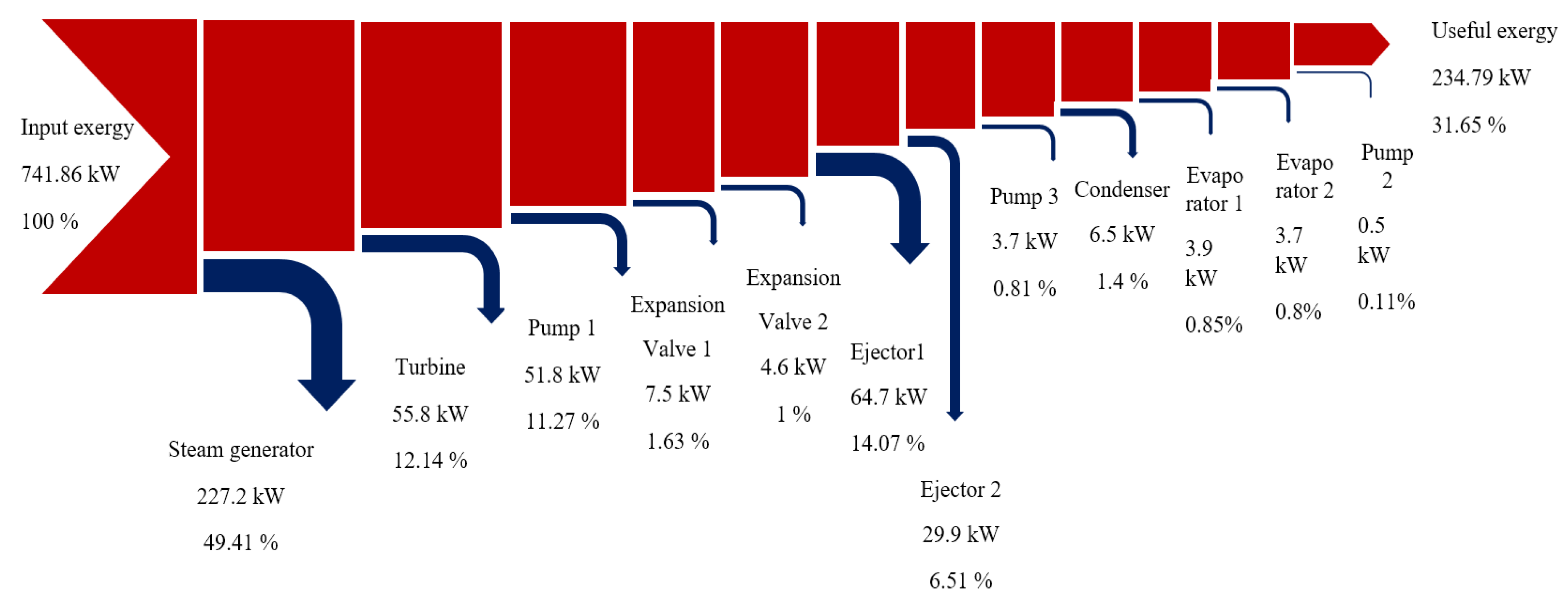
| Exergy efficiency (%) | 31.65 |
| Total product unit cost, USD/GJ | 48.40 |
| T | P | m | H | S | e | c | |||
|---|---|---|---|---|---|---|---|---|---|
| [K] | [bar] | [kg·s−1] | [kJ·kg−1] | [kJ·(kg·K)−1] | [kJ·kg−1] | [kW] | (USD/GJ) | (USD/h) | |
| 1 | 317.45 | 180 | 15 | 290.04 | 1.25 | 228.69 | 3430.3 | 15.54 | 191.79 |
| 2 | 404.15 | 180 | 15 | 500.84 | 1.84 | 263 | 3945 | 13.99 | 198.59 |
| 3 | 388.24 | 150 | 3 | 491.11 | 1.84 | 253.27 | 759.82 | 13.99 | 38.248 |
| 4 | 339.95 | 74.635 | 3.9 | 476.93 | 1.89 | 222.95 | 869.49 | 17.22 | 53.856 |
| 5 | 298.15 | 64.342 | 10 | 274.78 | 1.25 | 213.43 | 2134.3 | 13.99 | 107.44 |
| 6 | 298.5 | 65.758 | 10 | 274.98 | 1.25 | 213.62 | 2136.2 | 14.28 | 109.71 |
| 7 | 300.53 | 74.635 | 0.9 | 276.22 | 1.25 | 214.86 | 193.38 | 15.54 | 10.812 |
| 8 | 275.15 | 36.733 | 0.9 | 276.22 | 1.28 | 206.56 | 185.9 | 16.24 | 10.86 |
| 9 | 275.15 | 36.733 | 0.9 | 429.65 | 1.83 | 193.73 | 174.36 | 16.24 | 10.186 |
| 10 | 317.62 | 64.342 | 10 | 452.71 | 1.84 | 214.87 | 2148.7 | 13.99 | 108.16 |
| 11 | 300.53 | 74.635 | 15.9 | 276.22 | 1.25 | 214.86 | 3416.3 | 15.54 | 191.01 |
| 12 | 300.53 | 74.635 | 15 | 276.22 | 1.25 | 214.86 | 3222.9 | 12.99 | 150.63 |
| 13 | 363.48 | 112.5 | 2 | 476.98 | 1.84 | 239.14 | 478.27 | 13.99 | 24.076 |
| 14 | 280.15 | 41.765 | 0.9 | 425.81 | 1.80 | 198.8 | 178.92 | 15.22 | 9.7983 |
| 15 | 280.15 | 41.765 | 0.9 | 274.98 | 1.27 | 208.5 | 187.65 | 15.22 | 10.276 |
| 16 | 298.5 | 65.758 | 0.9 | 274.98 | 1.25 | 213.62 | 192.26 | 14.79 | 10.228 |
| 17 | 298.5 | 65.758 | 12.9 | 274.98 | 1.25 | 213.62 | 2755.8 | 14.79 | 146.59 |
| 18 | 298.5 | 65.758 | 12 | 274.98 | 1.25 | 213.62 | 2563.5 | 14.19 | 130.83 |
| 19 | 300.53 | 74.635 | 12 | 276.22 | 1.25 | 214.86 | 2578.3 | 14.79 | 137.16 |
| 20 | 323.51 | 65.758 | 2.9 | 461.1 | 1.86 | 216.3 | 627.26 | 16.35 | 36.887 |
| 21 | 285 | 1 | 27.458 | 411.21 | 3.84 | 0.30061 | 8.254 | 0.00 | 0 |
| 22 | 280 | 1 | 27.458 | 406.18 | 3.82 | 0.57935 | 15.908 | 51.35 | 2.9385 |
| 23 | 290 | 1 | 26.987 | 416.24 | 3.86 | 0.11416 | 3.0808 | 0.00 | 0 |
| 24 | 285 | 1 | 26.987 | 411.21 | 3.84 | 0.30061 | 8.1127 | 93.16 | 2.7186 |
| 25 | 298 | 1 | 589.35 | 424.29 | 3.88 | 0 | 0 | 0.00 | 0 |
| 26 | 301 | 1 | 589.35 | 427.31 | 3.89 | 0.013621 | 8.0278 | 326.23 | 9.4206 |
| 27 | 414.15 | 3.7189 | 15.421 | 593.45 | 1.75 | 76.381 | 1177.9 | 1.18 | 4.9915 |
| 28 | 365.8 | 3.7189 | 15.421 | 388.42 | 1.22 | 28.275 | 436.04 | 1.18 | 1.8478 |
| Assumptions/Parameters | Value |
|---|---|
| Plant life span | 15 years |
| Interest rate | 12% |
| CRF | 0.147 |
| The average inflation rate of the operating and maintenance cost, | 2.5% |
| CELF | 1.165 |
| Full load operational time τ, annually | 7000 h |
| Component | |||||||
|---|---|---|---|---|---|---|---|
| (USD/h) | (USD/h) | (USD/GJ) | (USD/GJ) | (USD/h) | (USD/h) | (%) | |
| Evaporator 1 | 2.94 | 0.67 | 106.73 | 16.24 | 0.23 | 2.26 | 90.88 |
| Evaporator 2 | 2.72 | 0.48 | 150.20 | 15.22 | 0.20 | 2.24 | 91.73 |
| Condenser | 9.42 | 0.73 | 327.15 | 13.99 | 0.33 | 8.69 | 96.40 |
| Expansion valve 1 | 10.86 | 10.81 | 16.24 | 15.54 | 0.42 | 0.05 | 10.37 |
| Expansion valve 2 | 10.28 | 10.23 | 15.22 | 14.79 | 0.25 | 0.05 | 16.48 |
| Ejector 1 | 10.00 | 4.58 | 105.75 | 13.99 | 3.26 | 5.42 | 62.47 |
| Ejector 2 | 5.31 | 2.30 | 93.81 | 13.99 | 1.51 | 3.01 | 66.65 |
| Pump 1 | 41.16 | 30.10 | 55.18 | 32.28 | 6.02 | 11.06 | 64.76 |
| Pump 2 | 2.27 | 0.29 | 317.43 | 32.28 | 0.06 | 1.98 | 97.17 |
| Pump 3 | 6.32 | 2.15 | 118.45 | 32.28 | 0.43 | 4.17 | 90.64 |
| Turbine | 58.33 | 28.10 | 32.28 | 13.99 | 2.81 | 30.23 | 91.50 |
| Steam generator | 6.79 | 3.14 | 3.67 | 1.18 | 0.96 | 3.65 | 79.12 |
| Total | 31.40 | 3.14 | 48.40 | 1.17 | 1.94 | 72.83 | 97.41 |
| Exergy Efficiency (%) | Cost of the Product (USD/Gj) | Secondary Mass Flow Rate | Secondary Mass Flow Rate | Extraction Ratio | Steam Generator Pressure (bar) | Evaporator 1 Coefficient kWm−2K−1 | Evaporator 2 Coefficient kWm−2K−1 | Condenser Coefficient kWm−2K−1 | Steam Generator Coefficient kWm−2K−1 |
|---|---|---|---|---|---|---|---|---|---|
| 37.55 | 31.15 | 1.2 | 0.7 | 0.15 | 180.6 | 0.92 | 0.92 | 1.03 | 1.16 |
| Design Parameters | Base Case | Optimal Solution |
|---|---|---|
| Extraction ratio | 0.2 | 0.15 |
| Steam generator pressure (kPa) | 18,000 | 18,060 |
| Secondary mass flow rate | 0.9 | 1.2 |
| Secondary mass flow rate | 0.9 | 0.7 |
| Evaporator 1 coefficient | 0.9 | 0.92 |
| Evaporator 2 coefficient | 0.9 | 0.92 |
| Condenser coefficient | 1 | 1.03 |
| Steam generator coefficient | 1 | 1.16 |
| Energy efficiency | 15.68 | 13.7 |
| Evaporator cooling capacities Qtot (kW) | 273.7 | 289.77 |
| Net power output (kW) | 222.1 | 480 |
| Steam generator heat (kW) | 3161.9 | 5610.4 |
| Total exergy destruction (kW) | 459.6 | 756.7 |
| Destruction cost rate (USD/h) | 1.94 | 1.8 |
| Total exergy efficiency (%) | 31.64 | 37.55 |
| Total product unit cost (USD/GJ) | 48.38 | 31.15 |
Disclaimer/Publisher’s Note: The statements, opinions and data contained in all publications are solely those of the individual author(s) and contributor(s) and not of MDPI and/or the editor(s). MDPI and/or the editor(s) disclaim responsibility for any injury to people or property resulting from any ideas, methods, instructions or products referred to in the content. |
© 2023 by the authors. Licensee MDPI, Basel, Switzerland. This article is an open access article distributed under the terms and conditions of the Creative Commons Attribution (CC BY) license (https://creativecommons.org/licenses/by/4.0/).
Share and Cite
Hammemi, R.; Elakhdar, M.; Tashtoush, B.; Nehdi, E. Multi-Objective Optimization of a Solar Combined Power Generation and Multi-Cooling System Using CO2 as a Refrigerant. Energies 2023, 16, 1585. https://doi.org/10.3390/en16041585
Hammemi R, Elakhdar M, Tashtoush B, Nehdi E. Multi-Objective Optimization of a Solar Combined Power Generation and Multi-Cooling System Using CO2 as a Refrigerant. Energies. 2023; 16(4):1585. https://doi.org/10.3390/en16041585
Chicago/Turabian StyleHammemi, Rania, Mouna Elakhdar, Bourhan Tashtoush, and Ezzedine Nehdi. 2023. "Multi-Objective Optimization of a Solar Combined Power Generation and Multi-Cooling System Using CO2 as a Refrigerant" Energies 16, no. 4: 1585. https://doi.org/10.3390/en16041585
APA StyleHammemi, R., Elakhdar, M., Tashtoush, B., & Nehdi, E. (2023). Multi-Objective Optimization of a Solar Combined Power Generation and Multi-Cooling System Using CO2 as a Refrigerant. Energies, 16(4), 1585. https://doi.org/10.3390/en16041585