Prediction of Food Factory Energy Consumption Using MLP and SVR Algorithms

Abstract

The industrial sector accounts for a significant proportion of total energy consumption. Factory Energy Management Systems (FEMSs) can be a measure to reduce energy consumption in the industrial sector. Therefore, machine learning (ML)-based electricity and liquefied natural gas (LNG) consumption prediction models were developed using data from a food factory. By applying these models to FEMSs, energy consumption can be reduced in the industrial sector. In this study, the multilayer perceptron (MLP) algorithm was used for the artificial neural network (ANN), while linear, radial basis function networks and polynomial kernels were used for support vector regression (SVR). Variables were selected through correlation analysis with electricity and LNG consumption data. The coefficient of variation of root mean square error (CvRMSE) and coefficient of determination (R²) were examined to verify the prediction performance of the implemented models and validated using the criteria of the American Society of Heating, Refrigerating, and Air-Conditioning Engineers Guideline 14. The MLP model exhibited the highest prediction accuracy for electricity consumption (CvRMSE: 17.35% and R²: 0.84) and LNG consumption (CvRMSE: 12.52% and R²: 0.88). Our findings demonstrate it is possible to attain accurate predictions of electricity and LNG consumption in food factories using relatively simple data.

1. Introduction

1.1. Energy Consumption of the Industrial Sector

Global awareness of the seriousness of climate change caused by increasing greenhouse gas (GHG) emissions has risen, and there is an increasing need to reduce GHG emissions and energy consumption in various sectors [1]. According to the energy survey results from the Ministry of Trade, Industry, and Energy (MOTIE) published in 2022, the total energy consumption in South Korea in 2019 was 226,479,000 TOE, which was 1.7% higher than that in 2016.

Table 1. Energy consumption of the industrial sector (percent of the total energy consumed) in Korea.

	2013	2016	2019
Industrial sector	118,991,000 TOE (59.4% of total)	130,010,000 TOE (60.4% of total)	136,348,000 TOE (60.2% of total)

Source: MOTIE, 2022.

indicates that the energy consumption of the industrial sector in Korea was 136,348,000 TOE in 2019, accounting for over 60% of the national total energy consumption (Figure 1), i.e., an average annual increase of 1.6% from 2016 to 2019 [2].

The industrial sector represents a major increase in the proportion of total energy consumption; therefore, we must prepare measures to rationalize energy consumption. One of these measures can be Factory Energy Management Systems (FEMSs), discussed in Section 1.2.

1.2. FEMSs

Active energy management methods have been adopted in various sectors to reduce energy consumption instead of conventional passive energy management methods. Conventional passive energy management methods include minimizing energy consumption for heating and cooling using high-performance insulation materials and high-efficiency windows. In contrast, the active energy management method manages the current status of energy use in real time, going beyond the conventional method. It includes the application of energy management systems (EMSs), high-efficiency facilities, and the use of renewable energy. In this regard, there is growing interest in EMSs that apply various information and communication technologies (ICTs) [3]. EMSs perform energy consumption monitoring, analysis, prediction, and equipment/utility control in real time to maximize the efficiency of energy consumption. FEMSs enable integrated energy management within factories and have been considered in many workplaces [4].

Owing to this trend, a survey on the domestic EMS introduction status, published in 2014 by MOTIE and the National IT Industry Promotion Agency (NIPA), predicted that the FEMSs market in Korea would exhibit a high average annual growth rate of 28.4%, reaching KRW 1115.2 billion in 2020. However, the current industrial level falls far short of this prediction. Therefore, the government announced plans to reduce industrial sector GHG emissions by 8.1% compared to BAU by 2030, as well as the mandatory application of FEMSs to workplaces that consume more than 100,000 TOE of energy from 2025 through the third Energy Master Plan [5]. The government also accelerated research and development on artificial intelligence (AI)-based FEMSs by planning to expand support for the dissemination of FEMSs in connection with smart factories and support more than 3000 new small and medium-sized companies with emissions of less than 100,000 TOE until 2040 [6].

1.3. Research Purpose

FEMSs include various functions for efficient energy management; however, predicting the amount of energy consumed in the near or far future is one of the most basic steps in energy management. For FEMSs application, this study predicted the electricity consumption (electrical energy) and liquefied natural gas (LNG) consumption (thermal energy) of a food factory using four ML algorithms: MLP, SVR-linear, SVR-RBF, and SVR-polynomial. The algorithms were utilized to obtain predicted values based on the available data. Machine learning-based energy consumption prediction can attain accurate predictions using available data. This study aims to select a model with the highest accuracy in predicting electricity and LNG consumption. This study derives a model with high prediction accuracy through model evaluation. The optimal model, derived through a series of steps, can be applied to FEMSs in the future to enable more efficient energy management in the target food factory.

1.4. Background

The purpose of this study is to predict the energy consumption of the target food factory using ML algorithms. Therefore, we reviewed related previous studies. Comesaña [7] conducted research on thermal inertia for public library buildings in northern Spain using MLP and long short-term memory (LSTM) neural networks. They compared and analyzed prediction errors and the coefficient of variation of the root mean square error (CvRMSE) according to the number of time lags introduced into the model. They found that the accuracy was high when considering thermal lag, with errors of less than 15% for thermal demand and less than 2% for indoor temperature. Lee [8] conducted research on the prediction of heating energy consumption using ANN for residential buildings. The energy prediction results obtained through the ANN model achieved a CvRMSE value ranging from 3.0 (in the best case) to 38.2% (in the worst case), with an average of 7.3%. Yang and Park [9] predicted the electricity consumption of healthcare buildings using prediction models based on multiple linear regression, SVM, and ANN, as well as MATLAB (Matrix Laboratory) and R programming. The ANN model exhibited the best performance, with an average root mean square error (RMSE) value of 153.2. Choi and Shin [10] predicted the electricity load of a store building using LSTM and a recurrent neural network (RNN). For LSTM, the average error range value was approximately 0.26, and the average error for 30 times was as low as 0.29, confirming that the STM algorithm is suitable for learning and predicting clustered electricity data. Nam [11] predicted outdoor temperature and solar radiation using ANN and the cooling and lighting energy consumption of a university office located in Jeonju, Korea, using TRNSYS 18 (a building load calculation software program). When prediction simulation was performed through training for one to seven days, the error decreased with an increase in the training data. When the seven-day training data with the lowest error rate were used, the error rate of the cooling/heating energy consumption was 1.92%, and that of the cooling/heating energy and lighting energy consumption was 2.07% without the application of a cutting-edge envelope. With the application of the cutting-edge envelope, the error rate of the cooling/heating energy consumption was 2.08%, and that of the cooling/heating energy and lighting energy consumption was 1.93%. Jeon et al. [12] predicted the monthly electricity consumption of apartment complexes using MLP, SVR, and DNN; they identified a complex where the largest increase in electricity demand was predicted by visualizing the change in electricity consumption using a geographic information system (GIS). The prediction performance was evaluated using the RMSE and mean absolute percentage error (MAPE). They confirmed that the DNN model was the best-performing model, with an RMSE of 0.046 and MAPE of 11.905. Quan et al. [13] predicted energy data for office buildings using indoor environmental data and energy consumption data with missing data. The missing data were interpolated using the variable-length sliding window algorithm, which can generate sufficient training data even with a small amount of data. The prediction accuracy of conventional sliding algorithms, the sequence-to-sequence imputation model (SSIM), and the LSTM model were compared. The CvRMSE value was 23.758% for the 3-h prediction and 29.348% for the 6-h prediction when the SSIM model was applied. When the LSTM model was applied, the CvRMSE value was 39.539% for the 3-h prediction and 42.259% for the 6-h prediction. This confirmed that the prediction accuracy was highest when building energy consumption over three hours was predicted using the SSIM model.

Our analysis of previous studies confirmed that there had been significant research on predicting energy consumption in buildings, including residential, university, and commercial buildings, using various ML algorithms. Therefore, we can confirm what type of data is required to predict the energy consumption of a target building type. Additionally, most studies compare prediction performance using two or more machine learning algorithms. This can verify which algorithm is applied with high prediction accuracy. However, few studies have been conducted on factories.

2. Machine Learning Model Background

2.1. Machine Learning (ML)

Machine learning (ML) is a branch within the overall tree of AI that allows a computer to learn and make decisions based on the input data. It creates functions by finding the relationship between input and output variables. ML is a method to extract relationships from data and can be divided into supervised learning with labels in the training data and unsupervised learning with no labels. Supervised learning includes prediction and classification models, while unsupervised learning includes clustering models. A representative example of prediction models that correspond to supervised learning is a regression model, which expresses the relationship between features and labels as a function using labeled training data. In other words, it is a statistical technique that infers the influence of one or more variables (independent variables) on another variable (dependent variable). Representative examples of classification models include k-nearest neighbor, support vector machine (SVM), and decision tree models [14,15].

Recently, research on data analysis using AI and ML-based prediction to process and analyze vast amounts of data has been conducted in various fields. It has been applied in energy and the environment for building energy optimization and system control through energy consumption status analysis and demand prediction. This can train a model using available data [7] and is highly efficient in optimally operating building energy using more advanced methods than conventional methods [9].

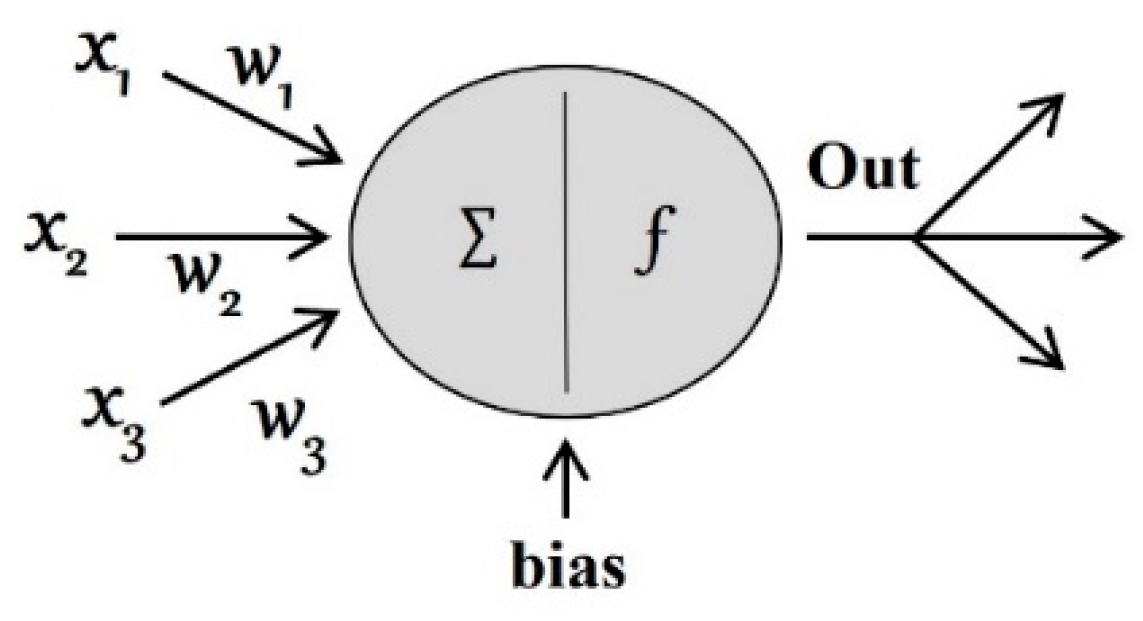
2.2. Artificial Neural Network (ANN)

Within ML, one of the most prominent techniques is the artificial neural network (ANN). ANN is a computational model consisting of input, hidden, and output layers that implement interactions when complex calculations are performed through artificial neurons based on biological neurons [16,17]. Training is performed by adding weights through the nodes between the input and target variables [9]. Adaptive control is possible because continuous training can be performed using the difference between the calculated result and actual value [18]. Feed-forward neural networks (FFNNs) or backpropagation neural networks (BPNNs), mainly referred to as a multilayer perceptron (MLP), are the most commonly used neural network structures [16].

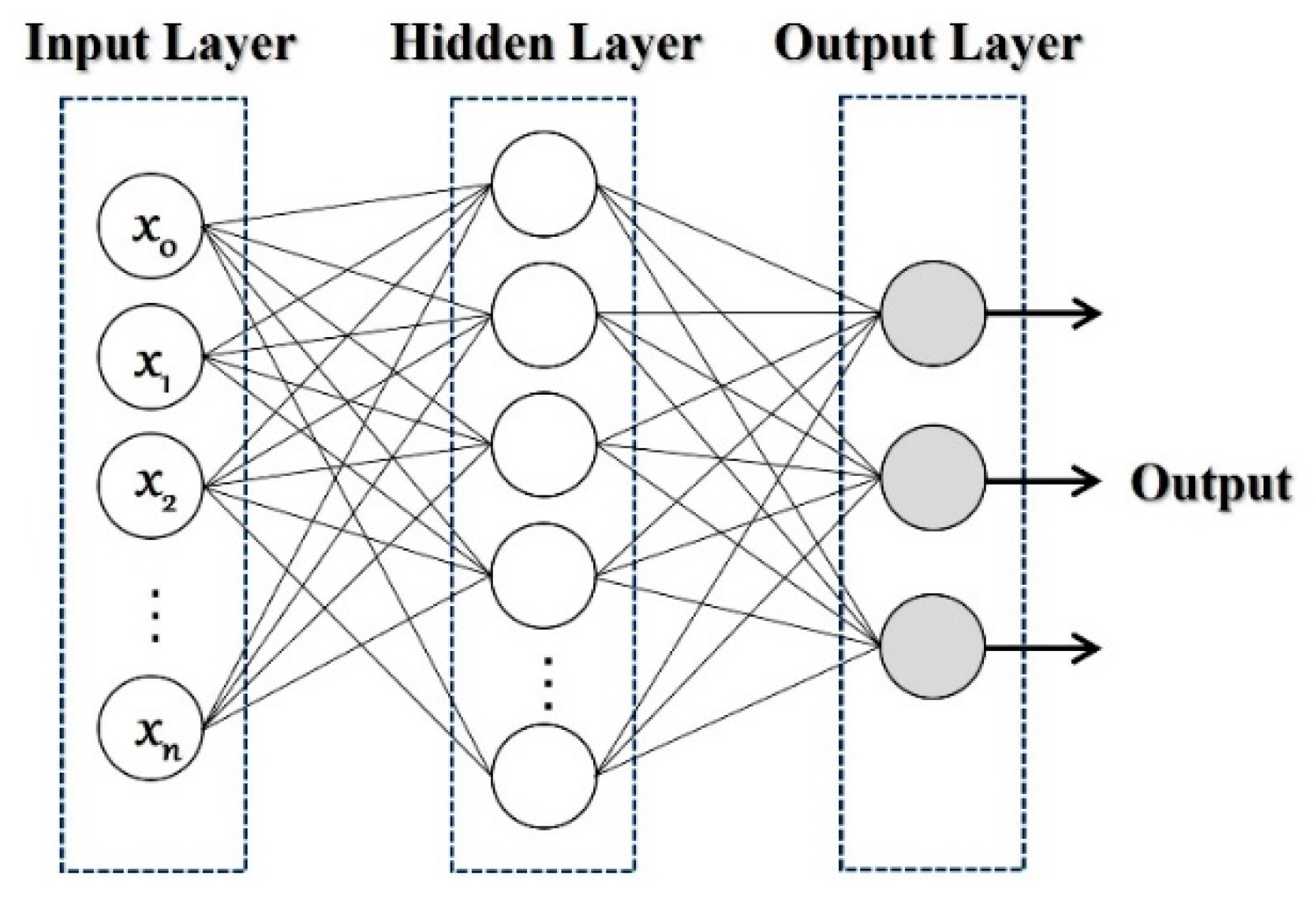
2.3. Multilayer Perceptron (MLP)

The structure of input and output layers of data is referred to as a single-layer perceptron. Figure 2 shows the structure of the perceptron.

In contrast, MLP is a sequential attachment of several layers composed of the perceptron. There is a hidden layer between the input and output layers. Figure 3 shows the structure of the MLP.

The calculation result of the perceptron can be expressed as follows:

$$f\left(b+x_1{w}_1+x_2{w}_2+x_3{w}_3\right)=f\left(b+\sum x_i{w}_i\right)$$

(1)

where b is the bias, x is the input, and w is the parameter of the perceptron. Learning adjusts the desired output for x by optimizing the given x value while changing the weight. This weight adjustment process starts with the correct answer and output calculation result and returns to the input terminal to adjust the weight value, i.e., “backpropagation”. In the perceptron, results are produced using activation functions. A single-layer perceptron contains only one activation function. Less accuracy is obtained for nonlinearly separable data. For the MLP, however, a higher accuracy can be obtained for nonlinearly separable data due to the hidden layer. ANNs that contain multiple hidden layers are referred to as deep neural networks (DNNs), and algorithms that train DNNs are referred to as deep learning. For the MLP, results are calculated using the weights of the input data and activation functions; this process is repeated until the output layer is reached. The weights and biases of each layer are calculated for data training.

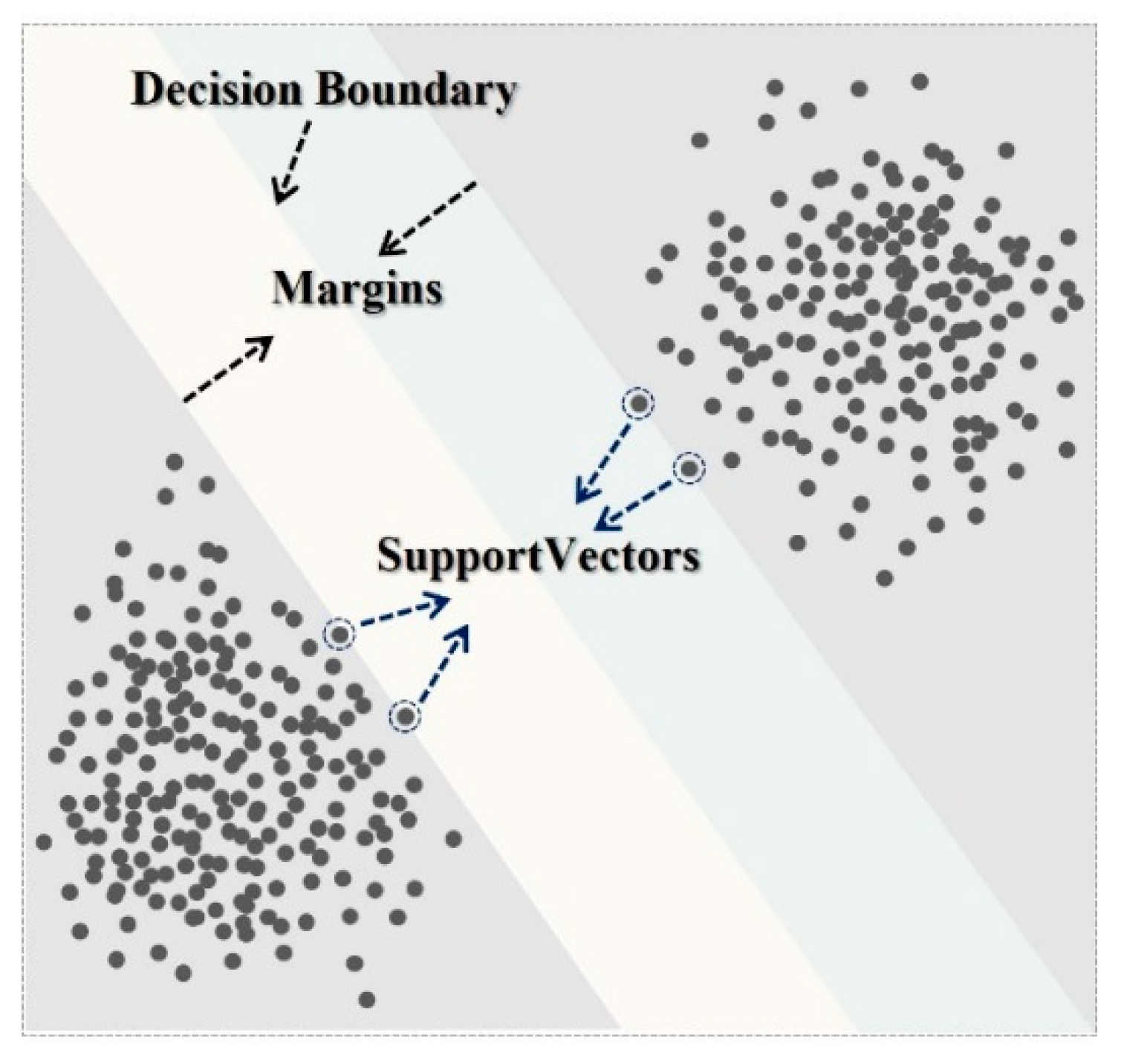
2.4. Support Vector Regression (SVR)

SVM, an ML method, is an algorithm for classifying the given data [9], wherein the SVR algorithm is used for regression. SVM is a method of prediction that defines the decision boundary of the given data and performs training, maximizing the distance to each support vector, i.e., the margin between classes. When it is assumed that training data are provided as $\left\{(x_i,y_i),\dots ,(x_N,y_N)\right\}\subset \chi \times R$, $ϵ$-SVR, as proposed by Vapnik [19], finds a function f(x) that is within the maximum deviation of $ϵ$ (intensive parameter) from the actual target values, $y_i$, for all training data, where $\omega$ is as small as possible. Here, $x$ is the input vector, $y$ is the output vector, $N$ is the number of training data, and $\chi$ is the input space, $R^m$. Training data errors smaller than $ϵ$ are neglected. The linear function can be expressed as follows [20]:

$$f\left(x\right)=\langle \omega ,x\rangle +bwith\omega \in \chi ,b\in R$$

(2)

where $〈\omega ,x〉$ represents the inner product in the input space and $\omega$ is the margin between the two support vectors. To find the smallest $\omega$, the following convex optimization problem can be constructed [20,21]:

$$minimize \frac{1}{2}\Vert {\omega }^2\Vert +C{\displaystyle \sum }_{i=1}^N\left({\xi }_i+{\xi }^{*}{}_i\right)$$

(3)

$$subject to \left\{\begin{array}{c}{y}_i-\langle \omega ,x_i\rangle -b\le ϵ+{\xi }_i\\ \langle \omega ,x_i\rangle +b-y_i\le ϵ+{\xi }_i\\ {\xi }_i, {\xi }^{*}{}_i\ge 0 \end{array}\right.$$

(4)

where ${\xi }_i\mathrm{and}{\xi }^{*}{}_i$ are slack variables, which allow the convex optimization problem to be established despite the presence of training data outside the deviation, and C is a normalized constant used to balance the empirical risk with the normalization term. C and $ϵ$ are the parameters determined by the user.

SVR is a technique for predicting data by finding the optimal hyperplane that contains as much data as possible within the margin; it has been used in various prediction fields, including demand prediction [22,23,24]. Figure 4 shows the concept of SVR. SVR is a linear prediction technique; training with data is performed in high-dimensional space rather than the original space, using a mapping function to predict diverse and nonlinear data [22]. As the amount of computation is significantly large in the high-dimensional expression process, a kernel function that enables the kernel trick is used. Using a kernel function can reduce the amount of computation required for the transformation and inner product of support vectors while preventing disturbance and overfitting between vectors. Representative kernel functions include linear, radial basis function (RBF), Gaussian, polynomial, and sigmoid. The SVR algorithm that uses a kernel function can be expressed as the following optimization problem [20]:

$$maximize \left\{\begin{array}{c}-\frac{1}{2}{\displaystyle {\displaystyle \sum }_{i,j=1}^N}\left({\alpha }_i+{\alpha }^{*}{}_i\right)\left({\alpha }_j+{\alpha }^{*}{}_j\right)k\left(x_i+x_j\right)\\ -ϵ{\displaystyle {\displaystyle \sum }_{i=1}^N}\left({\alpha }_i+{\alpha }^{*}{}_i\right)+{\displaystyle {\displaystyle \sum }_{i=1}^N}\left({\alpha }_i-{\alpha }^{*}{}_i\right) \end{array}\right.$$

(5)

$$subject to\left\{\begin{array}{c}{\displaystyle {\displaystyle \sum }_{i=1}^N}\left({\alpha }_i-{\alpha }^{*}{}_i\right)=0\\ {\alpha }_i,{\alpha }^{*}{}_i\in \left[0,C\right]\end{array}\right.$$

(6)

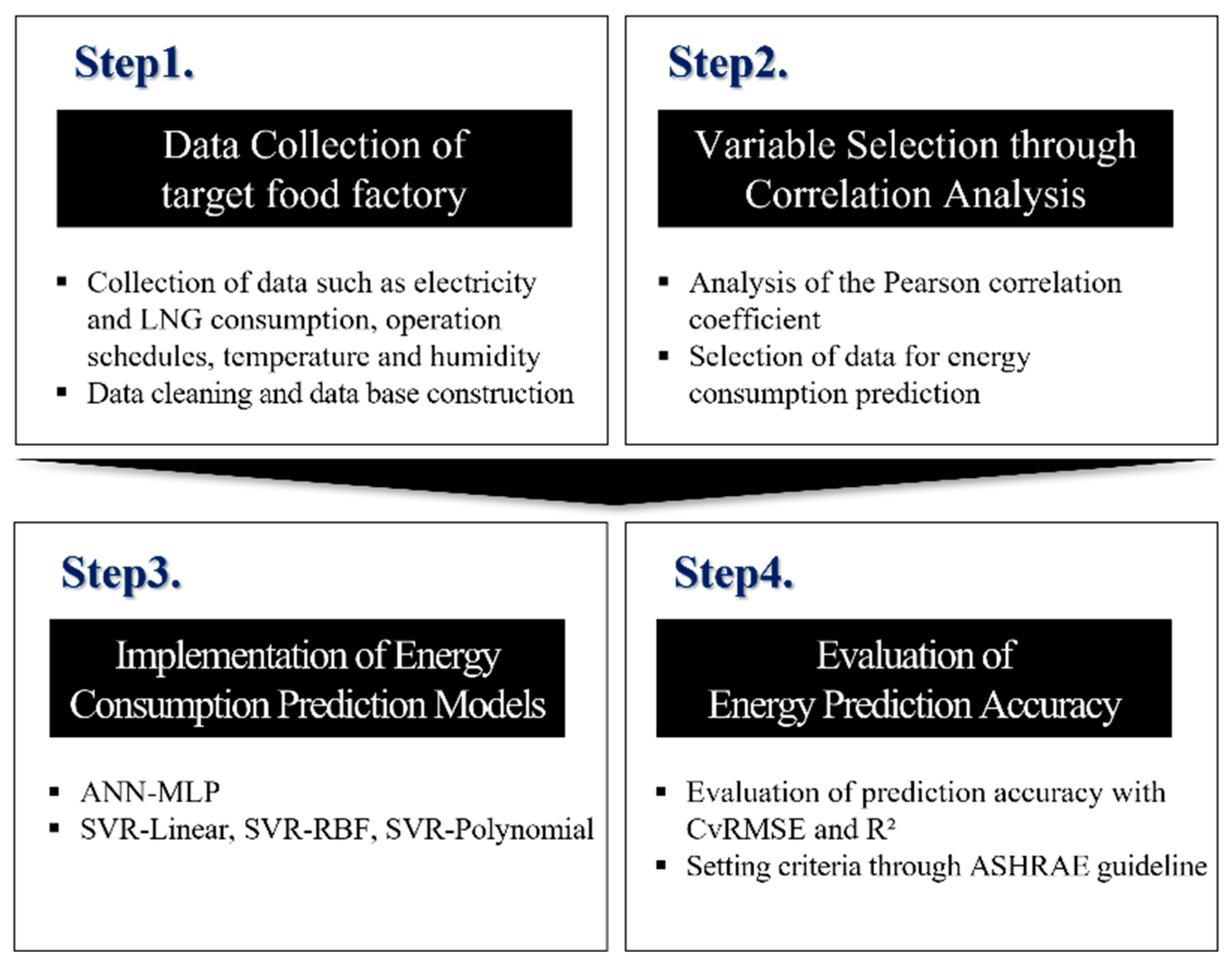
3. Materials and Methods

The research method can be mainly divided into the following four steps: (1) collection of data from the target food factory, (2) selection of data used in energy consumption prediction models through correlation analysis, (3) implementation of energy consumption prediction models, and (4) model evaluation. Figure 5 shows the research process.

3.1. Data Collection

The target of this study was a food factory in Korea that manufactures meat products, frozen foods, and smoked products. It conducts the following main processes: raw material pretreatment, smoking, baking, and sterilization. Energy is consumed by the specific systems used in each process; air conditioning for maintaining a constant temperature at the work site and freezer operations to maintain temperatures for refrigeration and storage freezer warehouses.

Most food factories in Korea are small or medium-sized, and few are equipped with old measurement and monitoring systems. Even for factories equipped with measuring instruments or control processes for each process, many are operated passively based on experience or intuition without considering energy consumption and any operating standards. The target food factory was not equipped with measuring instruments for each process, and energy was not properly managed. Therefore, measurement infrastructure, including the temperature, pressure, and stream flow rate, was constructed to collect energy production and consumption data. The communication module and Programmable Logic Controller were connected. Additionally, data monitoring and collection were performed using CIMON, a commercial Human Machine Interface (HMI) tool.

In predicting electricity consumption, daily data from 1 January 2018 to 31 December 2020 were used. The data included product production, operation schedule (input time and workforce), outdoor temperature, outdoor humidity, and electricity consumption from the previous day. For the product production and operation schedule data, the contents of the daily production reports of the target food factory were utilized through data cleaning and database construction. Temperature and humidity data from where the target food factory was located were provided by the Korea Meteorological Administration for the area (Yeongju, South Korea). Power planner data from the Korea Electric Power Corporation were used for electricity consumption.

For the prediction of LNG consumption, daily data from 6 December 2021 to 19 March 2022 were used. The data included product production, LNG temperature and pressure from the previous day, LNG flow rate from the previous day, outdoor temperature, outdoor humidity, and LNG consumption from the previous day. LNG-related data were constructed through data cleaning and database construction from daily boiler records manually prepared in the target food factory and HMI data.

Table 2. Data used.

Measurement Data	Production Data	Electricity Data	External Environment Data
LNG consumption LNG flow rate/temperature/pressure	Product production Input time Input workforce	Electricity consumption	Outdoor temperature Outdoor humidity

lists the data used in this study.

3.2. Variable Selection

Prior to the prediction of electricity and LNG consumption, correlations between the secured data and energy consumption were analyzed using Pearson’s correlation coefficient.

For correlation analysis, the linear relationship between two variables was analyzed. The two variables could be independent or correlated, and the intensity of the relationship between them was identified by the correlation coefficient, which ranges from −1 to 1. A value closer to 1 indicates a strong positive relationship, a value closer to −1 represents a strong negative correlation, and a value closer to zero indicates a weak correlation.

Pearson’s correlation coefficient for a population was calculated as follows:

$$r=\frac{{{\displaystyle \sum }}_{i=1}^n\left(X_i-\overline{X}\right)\left(Y_i-\overline{Y}\right)}{\sqrt{{{\displaystyle \sum }}_{i=1}^n{\left(X_i-\overline{X}\right)}^2}\sqrt{{{\displaystyle \sum }}_{i=1}^n{\left(X_i-\overline{X}\right)}^2}}$$

(7)

where $r$ is Pearson’s correlation coefficient, n is the number of variables, and $\overline{X}$ and $\overline{Y}$ are the averages of each variable.

There is no standard for the interpretation of the correlation coefficient, and the interpretation method may vary depending on situations, such as data characteristics and the representativeness of samples. Rea and Parker [25] reported almost no correlation for the absolute correlation coefficient value range of 0.0 to 0.1, a weak correlation from 0.1 to 0.2, a moderate correlation from 0.2 to 0.4, a relatively strong correlation from 0.4 to 0.6, a strong correlation from 0.6 to 0.8, and a very strong correlation from 0.8 to 1.0. Therefore, energy consumption was predicted after excluding data with a correlation coefficient between 0.0 and 0.1.

3.3. Implementation of Energy Consumption Prediction Models

In this study, the electricity and LNG consumption prediction performance was compared using ANN and SVR, which are algorithms commonly used for energy and environmental predictions [12,26,27]. The MLP algorithm, which is the most commonly used ANN, was utilized [12]. Linear, RBF, and polynomial kernels were used for SVR.

The prediction models were implemented and analyzed in Python 3.9.7, Tensorflow 2.3.0, Keras 2.4.3, Sklearn 1.0.2, Pandas 1.4.1, Numpy 1.19.5, and Matplotlib 3.5.1 environments. Of the collected data, 90% were set as the training set, and the remaining 10% were set as the test set for performance verification. In the MLP-based analysis, the main hyperparameters were set to be ReLu for the activation function for the hidden layer, adam for the solver for weight optimization, 0.9 for the momentum, constant for the learning rate, 0.001 for the initial learning rate, and 100 for the hidden layer size, which corresponded to default. For the SVR-based analysis, the error tolerance (epsilon, $\epsilon$) was set to 0.1, the degree of the polynomial kernel to 3, the gamma of the RBF and polynomial kernel to scale, which corresponded to default, and C was set to 100. Minmax Scaling and Standard Scaling were applied simultaneously to preprocess the variables used in the energy consumption prediction.

Minmax Scaling is a data normalization method to set the minimum value of a dataset to zero and the maximum value to 1. It is achieved by dividing the value obtained by subtracting the minimum value of the measurement data from the data by the value obtained by subtracting the minimum value from the maximum value of the measurement data:

$$X_{minmax}=\frac{x-x_{min}}{x_{max}-x_{min}}$$

(8)

where $x_{min}$ is the minimum value of the measurement data, and $x_{max}$ is the maximum value of the measurement data.

Standard Scaling is a method of standardizing data with a mean value of zero and a variance of 1, achieved by dividing the value obtained by subtracting the mean value of the measurement data from the data by the standard deviation of the measurement data:

$$X_{standard}=\frac{x-\mu }{s}$$

(9)

where $\mu$ is the mean value of the measurement data, and $s$ is the standard deviation of the measurement data.

3.4. Prediction Accuracy Evaluation

CvRMSE and the coefficient of determination, R² (R-squared, variance explained), were examined to verify the prediction performance of the implemented models. The validity of the models was verified based on the criteria of the American Society of Heating, Refrigerating, and Air-Conditioning Engineers (ASHRAE) Guideline 14 [11].

3.4.1. Coefficient of Variation of Root Mean Square Error (CvRMSE)

CvRMSE is a method of identifying the error between the predicted and actual data values based on error analysis through the degree of variance; the result is expressed as the error rate (%). CvRMSE is a percentage value of the RMSE. The RMSE and CvRMSE equations are as follows:

$$RMSE=\sqrt{\frac{\sum {\left({\widehat{y}}_i-y_i\right)}^2}{N}}$$

(10)

and

$$CvRMSE=\frac{RMSE}{\mu }\times 100=\frac{\sqrt{\frac{\sum {\left({\widehat{y}}_i-y_i\right)}^2}{N}}}{\mu }\times 100\left(\%\right)$$

(11)

where ${\widehat{y}}_i$ is the predicted value of the model, $y_i$ is the measured value, $N$ is the number of actual data, and $\mu$ is the average of the measurement data.

Table 3. Evaluation criteria for predictive models.

Category	Unit	CvRMSE
ASHRAE Guideline14	Monthly	<10%
	Hourly	<30%
Target value	Daily	<20%

lists the prediction model evaluation criteria through CvRMSE when the monthly and hourly data presented by the ASHRAE Guideline [28] were used. As daily data were used in this study, the target value was set to 20%, which is the median value of the monthly and hourly criteria presented by ASHRAE.

3.4.2. Coefficient of Determination, R²

R² is a variance-based prediction performance evaluation index commonly used in regression and statistical analyses. R² can be obtained by dividing the explained sum of squares (ESS, also SS due to Regression) by the total sum of squares (TSS). It can also be obtained by subtracting the value obtained by dividing the residual sum of squares (RSS, SS due to Residual) by TSS from 1:

$$R^2=\frac{ESS}{TSS}=1-\frac{RSS}{TSS}=\frac{{{\displaystyle \sum }}_{i=1}^n{\left(y_i-{\widehat{y}}_i\right)}^2}{{{\displaystyle \sum }}_{i=1}^n{\left(y_i-{\overline{y}}_i\right)}^2}$$

(12)

where $ESS$ is the sum of the squares of the difference between each predicted value of Y and the mean value, representing the degree that the model cannot explain the variation of the target value, Y; $TSS$ is the sum of the squares of the difference between each actual value of Y and the mean value, representing the variation in the target value, Y; $RSS$ is the sum of the squares of the difference between each actual value of Y and the predicted value of that value, representing the degree that the model cannot explain the variation of the target value, Y; and ${\overline{y}}_i$ is the mean value of $y$.

The correlation is weaker the closer the value of R² is to 0 and stronger the closer it is to 1. The appropriate criterion presented by ASHRAE is 0.8. Therefore, 0.8 was set as the target value for prediction model performance.

4. Results and Discussion

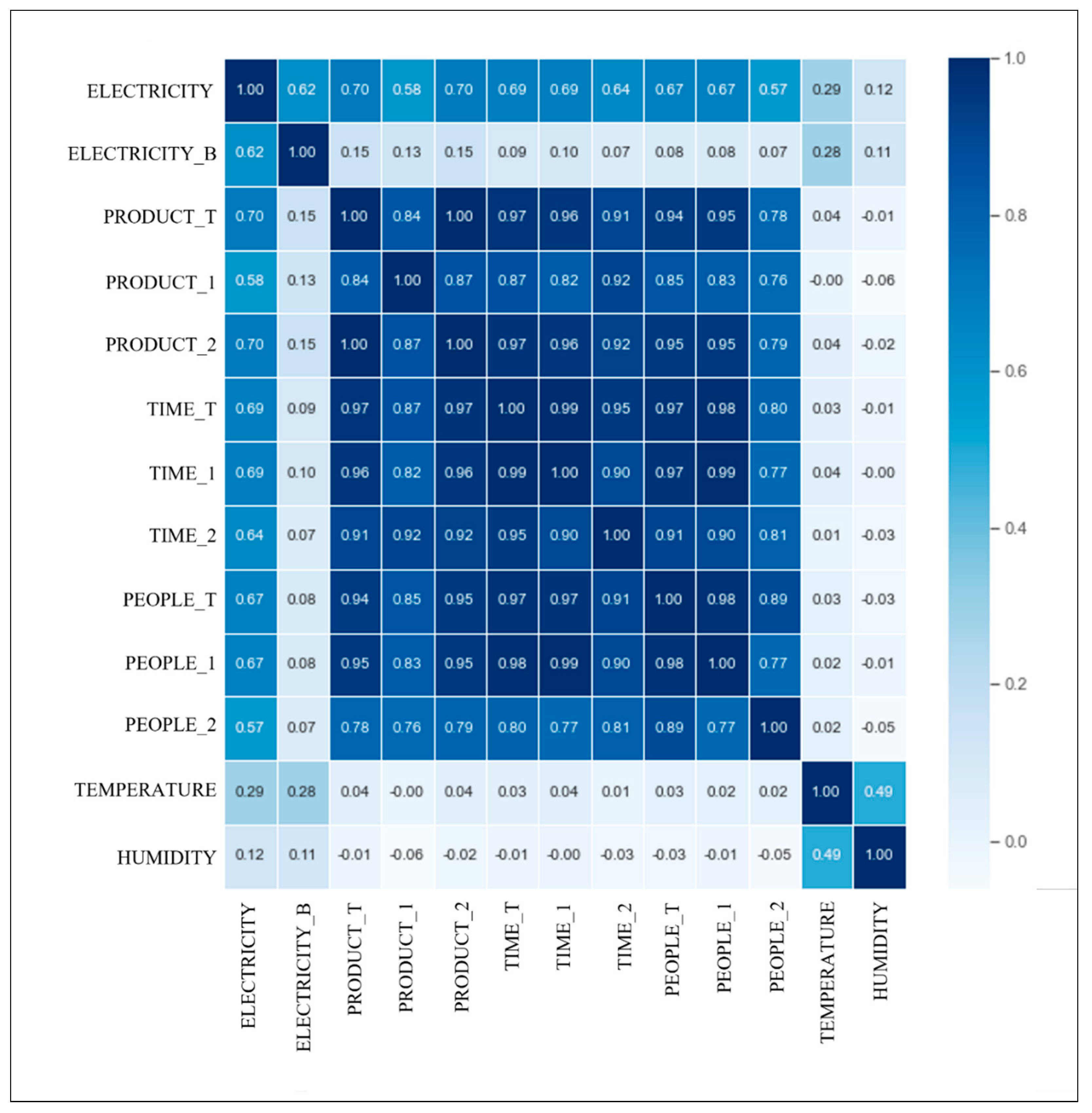
4.1. Variable Selection Results

Table 4. Data for electricity consumption prediction.

Category	Data Type	Notation
Electricity consumption	Electricity consumption of the day	ELECTRICITY
	Electricity consumption of the previous day	ELECTRICITY_B
Product production	Total product production	PRODCUT_T
	Product production in factory 1	PRODUCT_1
	Product production in factory 2	PRODUCT_2
Input time	Total input time	TIME_T
	Input time in factory 1	TIME_1
	Input time in factory 2	TIME_2
Input workforce	Total input workforce	PEOPLE_T
	Input workforce in factory 1	PEOPLE_1
	Input workforce in factory 2	PEOPLE_2
External environment	Outdoor temperature	TEMPERATURE
	Outdoor humidity	HUMIDITY

lists the 13 types of data schema secured for the prediction of electricity consumption. The secured data included the electricity consumptions of the day and the previous day, total product production, product production in factories 1 and 2, total input time, input time in factories 1 and 2, total input workforce, input workforce in factories 1 and 2, and outdoor temperature and humidity. The dependent variable was the electricity consumption of the day, and the remaining data were used as independent variables.

Here, product production in factory 1 included grilled meat products, hams, frankfurters, and smoked products, while product production in factory 2 included Vienna sausage products.

Pearson’s correlation coefficient between each variable and the electricity consumption of the day was displayed as a heatmap (Figure 6).

Table 5. Correlations with the electricity consumption of the day.

Notation	Correlation Coefficient
ELECTRICITY	0.62
ELECTRICITY_B	0.70
PRODCUT_T	0.58
PRODUCT_1	0.70
PRODUCT_2	0.69
TIME_T	0.69
TIME_1	0.64
TIME_2	0.67
PEOPLE_T	0.67
PEOPLE_1	0.67
PEOPLE_2	0.57
TEMPERATURE	0.29
HUMIDITY	0.12

lists the correlation coefficient with the electricity consumption of the day. Here, the total production and product production in factory 1 showed the greatest correlation with electricity usage (0.70). Additionally, there were very strong correlations between variables that corresponded to product production, input time, and input workforce. For example, input workforce in factory 2 had strong correlations with total product production (0.78), product production in factory 1 (0.76), product production in factory 2 (0.79), input time in factory 1 (0.77), and input workforce in factory 1 (0.77), and very strong correlations with the other variables. As all of the secured data had a correlation coefficient of 0.1 or higher, all were used for electricity consumption prediction.

Table 6. Data for LNG consumption prediction.

Category	Data Type	Notation
LNG consumption	LNG consumption of the day	LNG
	LNG consumption of the previous day	LNG_B
LNG flow rate/temperature/pressure	Total LNG flow rate of the previous day	LNG_FLOW_B_T
	Boiler 1 LNG temperature of the previous day	LNG_TEMPERATURE_B_1
	Boiler 2 LNG temperature of the previous day	LNG_TEMPERATURE_B_2
	Boiler 1 LNG pressure of the previous day	LNG_PRESSURE_B_1
	Boiler 2 LNG pressure of the previous day	LNG_PRESSURE_B_2
Product production	Total product production	PRODCUT_T
	Product production in factory 1	PRODUCT_1
	Product production in factory 2	PRODUCT_2
External environment	Outdoor temperature	TEMPERATURE
	Outdoor humidity	HUMIDITY

lists the 12 types of data schema secured for predicting LNG consumption. The secured data included LNG consumption of the day and the previous day, total LNG flow rate of the previous day, temperature and pressure of boilers 1 and 2 on the previous day, total product production, product production in factories 1 and 2, and outdoor temperature and humidity. The dependent variable was the LNG consumption of the day, and the remaining data were used as independent variables.

Pearson’s correlation coefficient between each variable and LNG consumption was displayed as a heatmap (Figure 7).

Table 7. Correlations with the LNG consumption of the day.

Notation	Correlations Coefficient
LNG_B	0.40
LNG_FLOW_B_T	0.39
LNG_TEMPERATURE_B_1	0.06
LNG_TEMPERATURE_B_2	−0.04
LNG_PRESSURE_B_1	−0.23
LNG_PRESSURE_B_2	−0.24
PRODCUT_T	0.93
PRODUCT_1	0.94
PRODUCT_2	0.79
TEMPERATURE	−0.04
HUMIDITY	0.04

lists the correlation coefficient with the LNG consumption of the day. Here, product production in factory 1 showed the greatest correlation with LNG consumption (0.94). Additionally, there was a strong correlation between the LNG consumption of the previous day and the total LNG flow rate of the previous day (0.96), between the LNG pressure of boiler 1 from the previous day and boiler 2 LNG pressure from the previous day (0.96), between the total product production and product production in factory 1 (0.82), between the total product production and product production in factory 2 (0.99), and between the product production in factory 1 and product production in factory 2 (0.89). There was also a strong correlation between the boiler 1 LNG temperature of the previous day and boiler 2 LNG temperature of the previous day (−0.60) and between the boiler 1 LNG temperature of the previous day and outdoor temperature (0.63).

Among the secured data, the boiler 1 LNG temperature of the previous day, boiler 2 LNG temperature of the previous day, outdoor temperature, and outdoor humidity had correlation coefficients of less than 0.1 with the LNG consumption of the day; these were thus excluded from the LNG consumption prediction.

4.2. Energy Consumption Prediction Results

Data were selected through correlation analysis to predict the electricity and LNG consumption of the target food factory. Based on the selected variables, electricity consumption and LNG consumption were predicted using MLP and SVR-linear, RBF, and polynomial kernels, and their accuracy was analyzed.

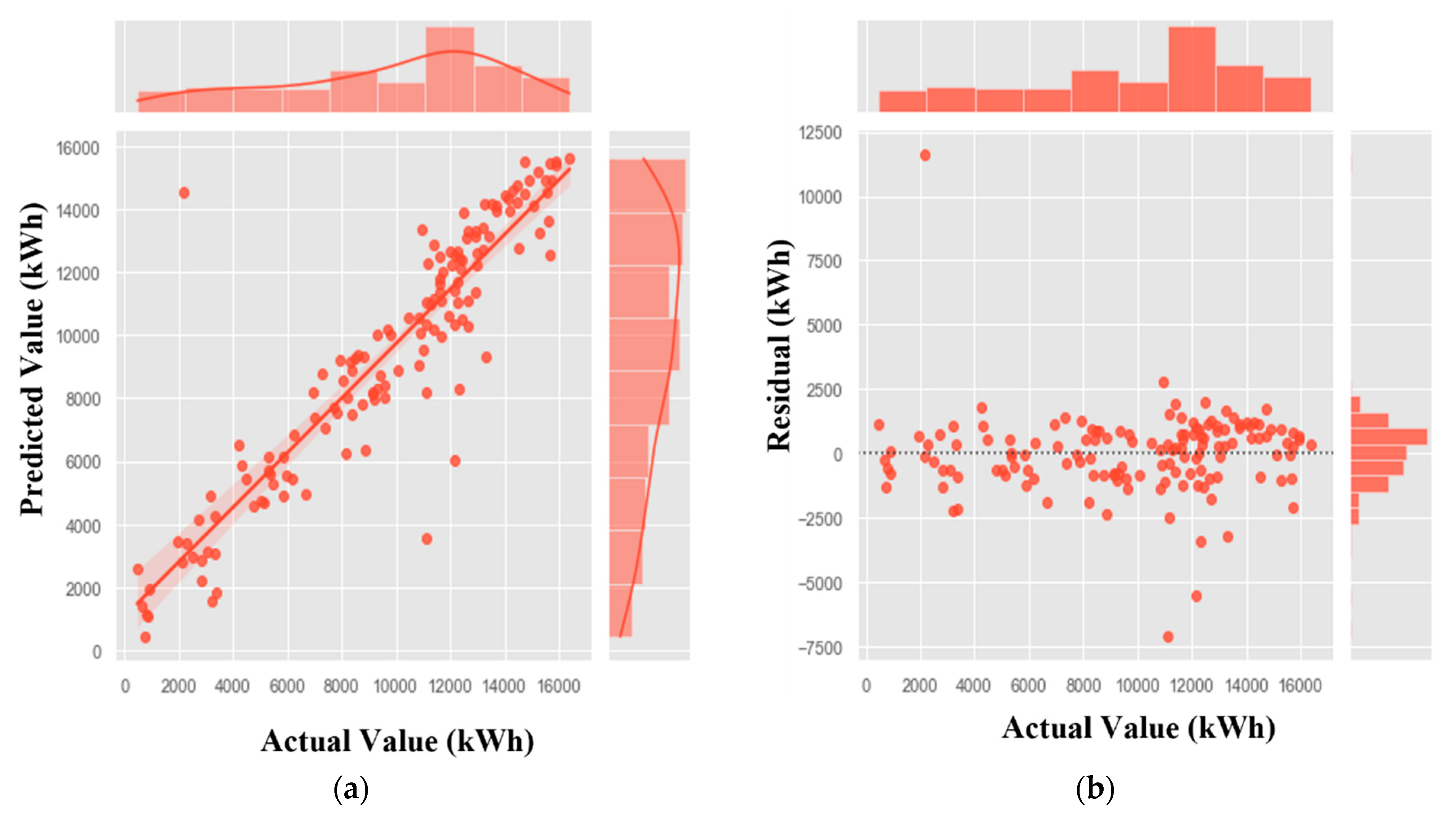
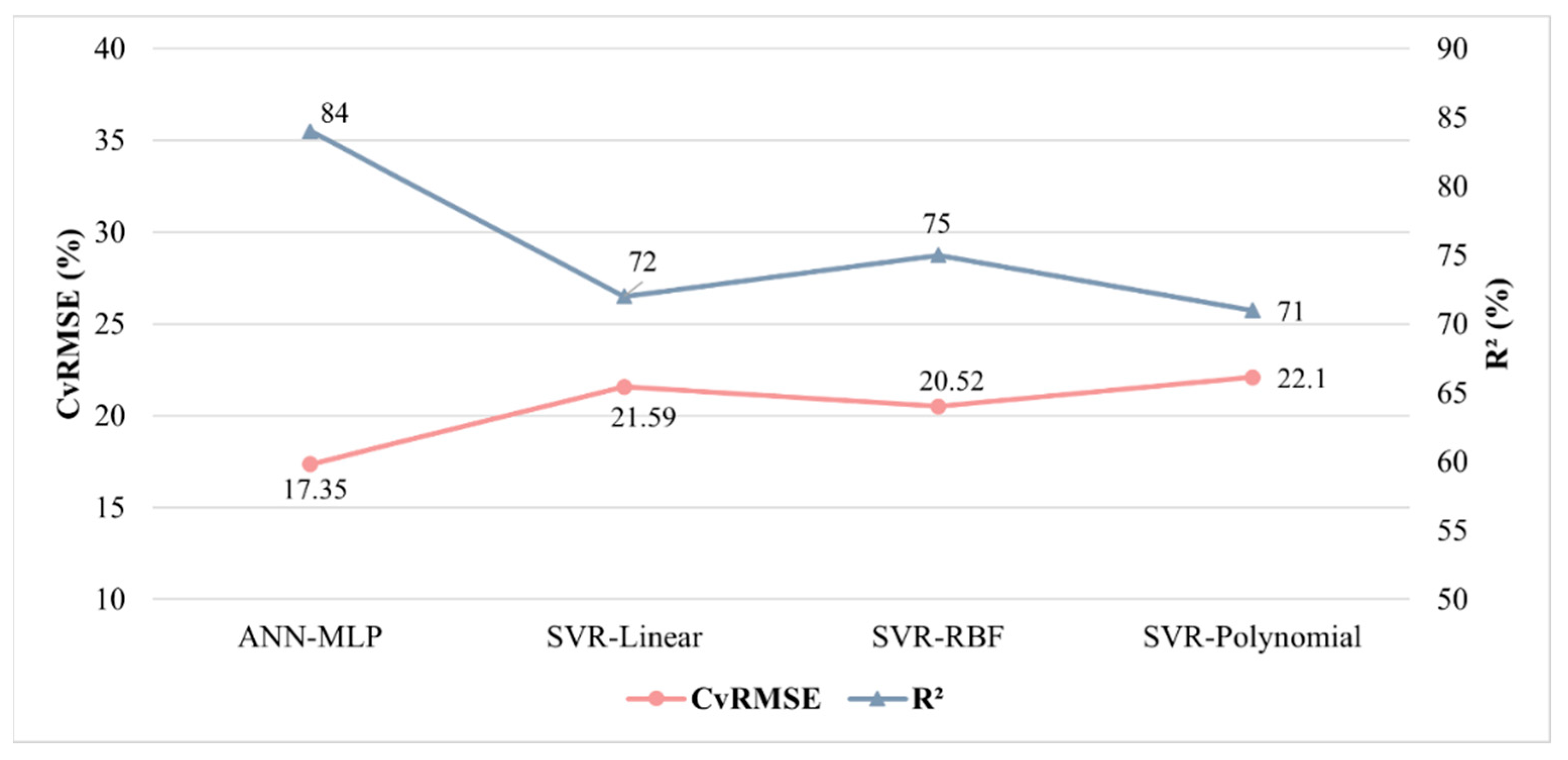
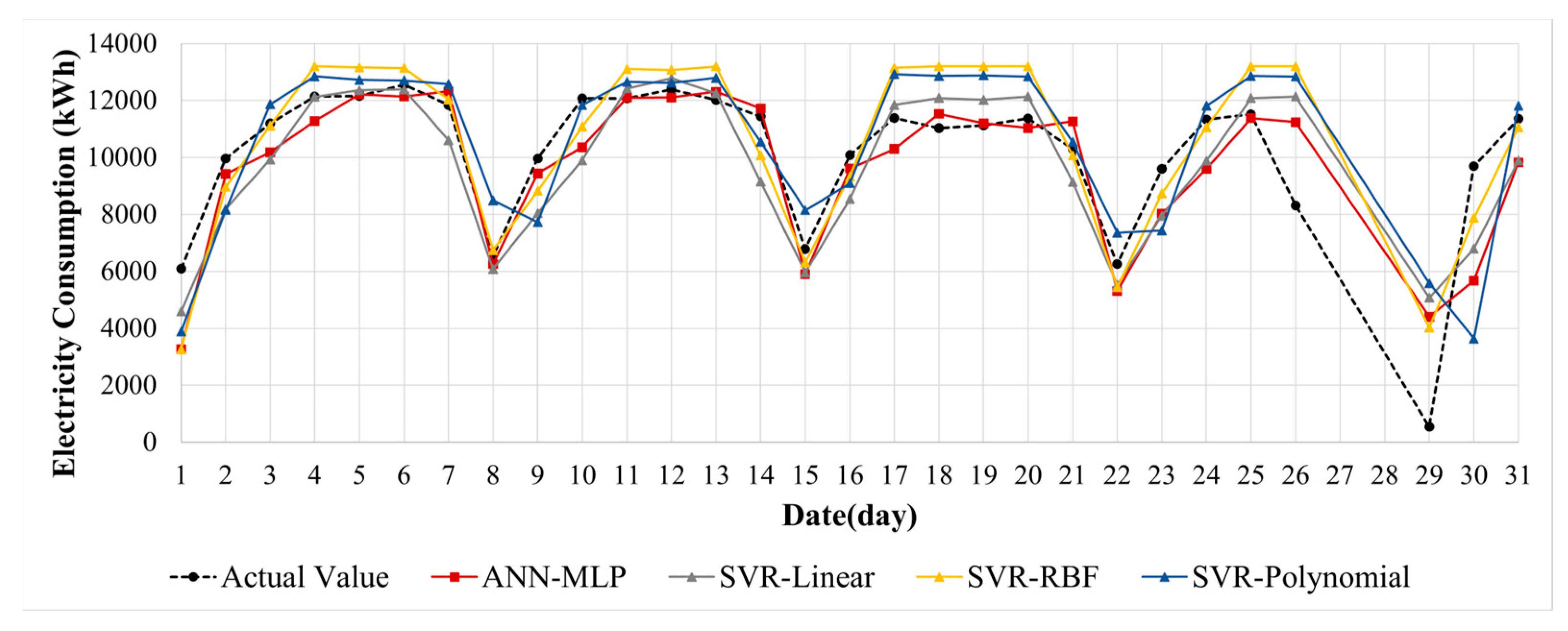
4.2.1. Electricity Consumption Prediction Results

When electricity consumption was predicted using MLP, a CvRMSE value of 17.35% and an R² value of 0.84 were obtained. Figure 5 visualizes the data distribution of the MLP-based electricity consumption prediction results using Jointplot. A linear regression line that shows the tendency of the data distribution of the electricity consumption prediction model occurs in the regression plot (Regplot) (Figure 8a). The degree of error in the data based on the regression line can be observed in the residual plot (Residplot) (Figure 8b). Regressopm plot (Regplot) and Residplot are statistical data visualization methods that can be used through the Seaborn Library.

Figure 9 visualizes the data distribution through the SVR’s linear, RBF, and polynomial kernels using the Matplot Library. The “+” mark in red represents the distribution of the measurement data, while gray indicates the regression line. On the x-axis, the dimension was reduced for visualization using the t-SNE module.

Figure 10 compares the CvRMSE and R² for each electricity consumption prediction model.

For the electricity consumption prediction, only the MLP model met the target values (CvRMSE: 20% and R²: 0.80). When the prediction results of the MLP model and three SVR models were compared, the MLP model exhibited the highest prediction accuracy, with a CvRMSE value of 17.35% and R² value of 0.84. Figure 11 compares the measured electricity consumption values with the values predicted by each model for one month (1 to 31 January 2017).

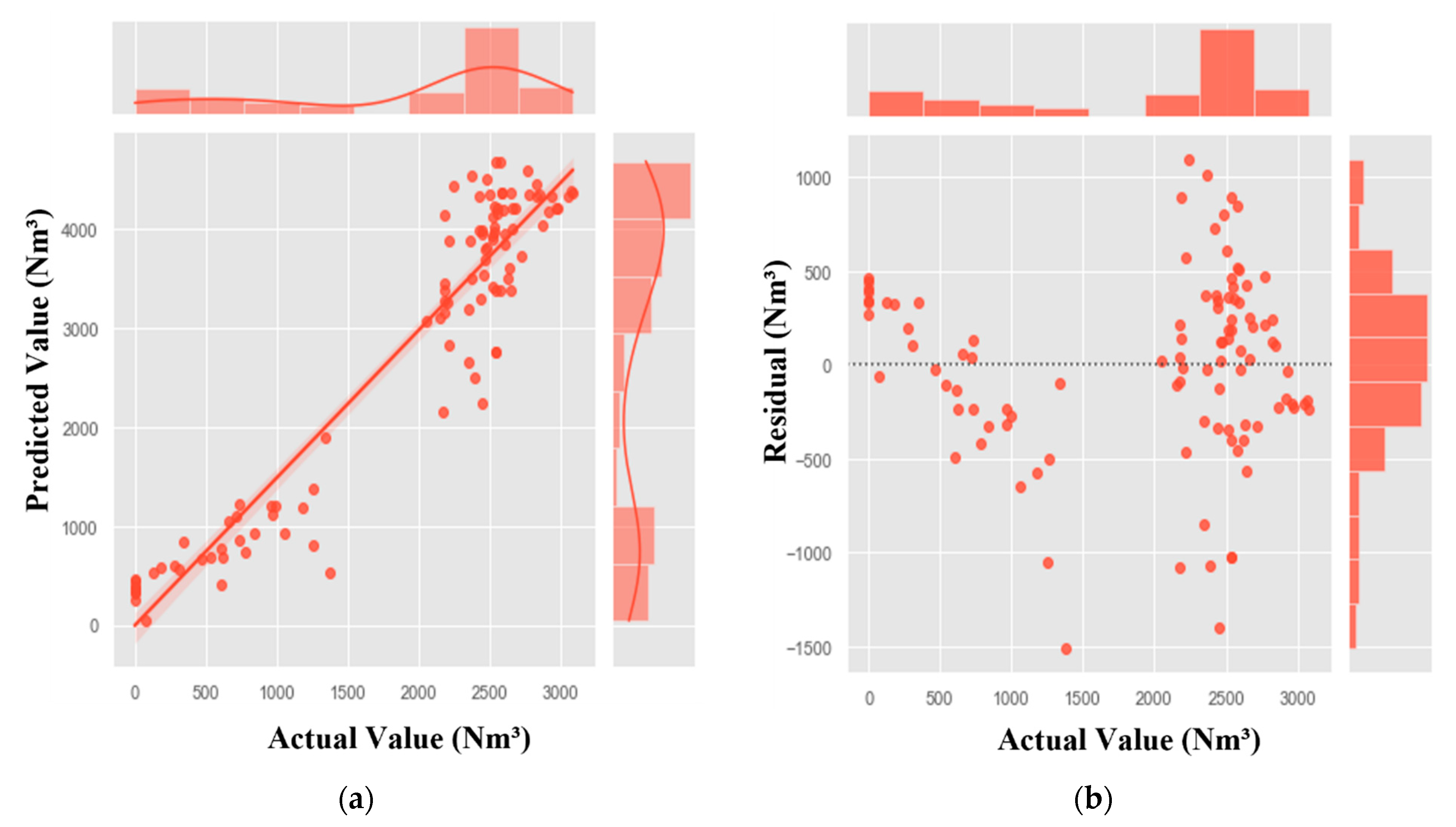
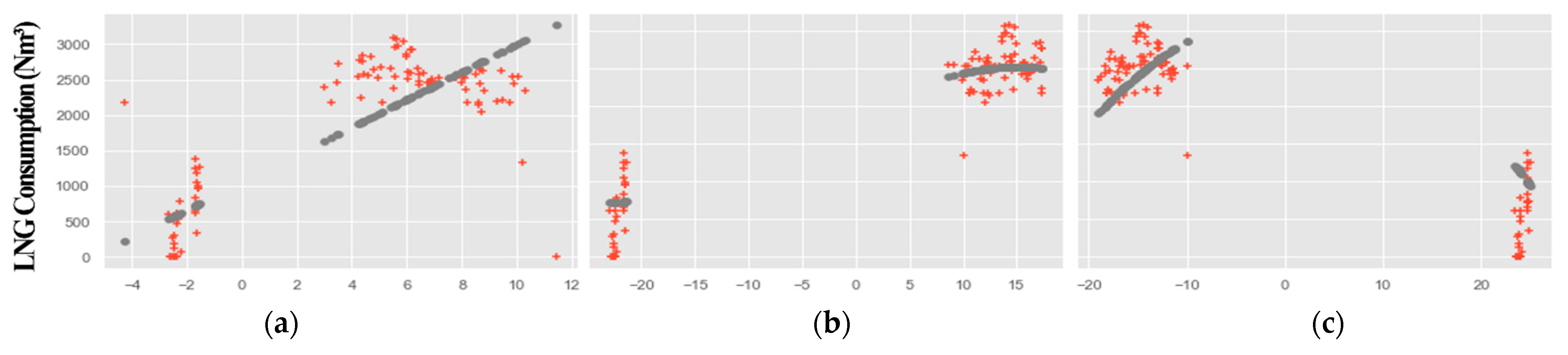
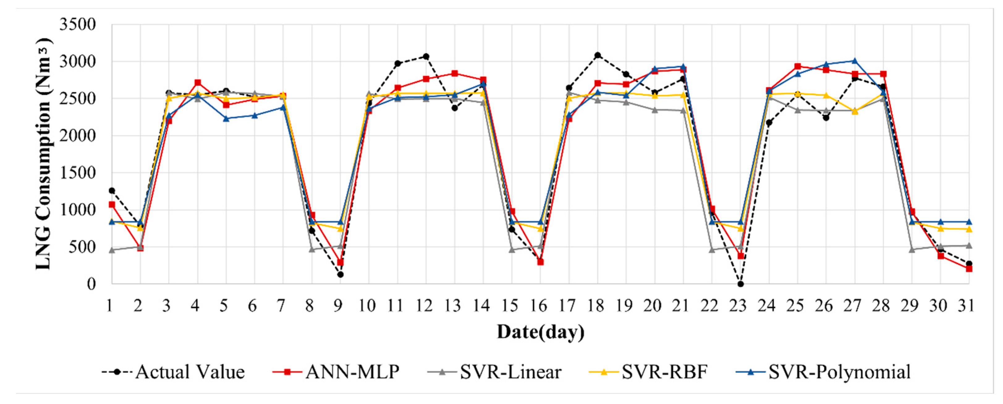
4.2.2. LNG Consumption Prediction Results

The MLP-based LNG consumption prediction results had a CvRMSE of 12.52% and an R² of 0.88. Figure 9 visualizes the data distribution of the MLP-based LNG consumption prediction results using Jointplot. A linear regression line that shows the tendency of the data distribution of the LNG consumption prediction model is shown in Regplot (Figure 12a), and the degree of error in the data based on the regression line is shown in Residplot (Figure 12b).

When LNG consumption was predicted using SVR, a CvRMSE value of 21.59% and an R² value of 0.82 were obtained for the linear kernel; a CvRMSE value of 17.01% and an R² value of 0.88 for the RBF kernel; and a CvRMSE value of 21.58% and an R² value of 0.82 for the polynomial kernel. The RBF kernel exhibited the highest accuracy among the three SVR kernels.

Figure 13 visualizes the data distribution through the linear, RBF, and polynomial kernels of the SVR using the Matplot Library. Many blanks occurred in the scatter graphs because a relatively small amount of data over approximately 3.5 months were used and numerous Nan values were included for the LNG consumption prediction. In contrast, data over about three years were used for the electricity consumption prediction.

Figure 14 compares the CvRMSE and R2 for each LNG consumption prediction model.

For the LNG consumption prediction, the MLP and SVR-RBF models satisfied the target value of the CvRMSE (20%), and all of the models (the MLP model and three SVR models) met the target value of the R² (0.80). The MLP model exhibited the highest prediction accuracy with a CvRMSE value of 12.52% and an R² value of 0.88. Figure 15 compares the measured LNG consumption values with the values predicted by each model for a month (1 to 31 January 2022).

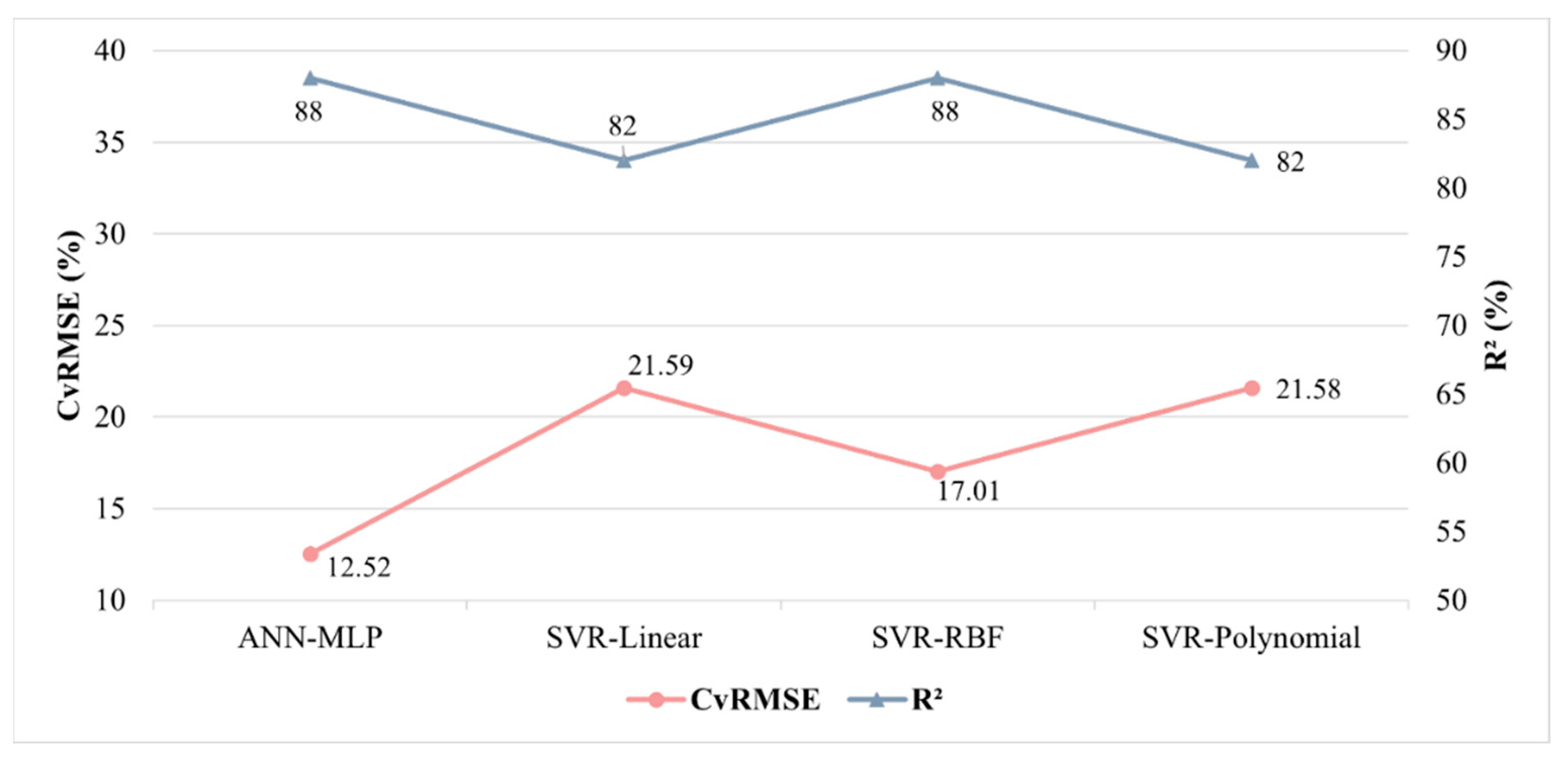
4.2.3. Energy Consumption Prediction Model Selection

Table 8. Evaluation of the prediction results for the MLP and SVR (linear, RBF, and polynomial).

		MLP	SVR
			Linear	RBF	Polynomial
Electricity	CvRMSE	17.35%	21.59%	20.52%	22.10%
	R2	0.84	0.72	0.75	0.71
LNG	CvRMSE	12.52%	21.59%	17.01%	21.58%
	R2	0.88	0.82	0.88	0.82

summarizes the CvRMSE and R² for eight cases (four electricity consumption prediction models and four LNG consumption prediction models). The MLP model exhibited the highest prediction accuracy in electricity consumption (CvRMSE: 17.35% and R²: 0.84) and LNG consumption (CvRMSE: 12.52% and R²: 0.88).

Therefore, based on the ASHRAE guideline, the MLP model was selected as the electricity and LNG consumption prediction model for the target food factory because it satisfied all of the set target values, exhibiting the highest prediction accuracy among the analysis cases.

5. Conclusions

This study aimed to select a model with the highest accuracy in predicting the electricity and LNG consumption of a food factory. The MLP, SVR-linear, SVR-RBF, and SVR-polynomial algorithms were utilized, and the prediction accuracy of each model was analyzed.

The main results of this study were as follows. (1) Product production had the highest correlation with electricity and LNG consumption. (2) The correlation coefficients of the LNG temperatures of boilers 1 and 2 on the previous day, outdoor temperature, and outdoor humidity with LNG consumption were less than 0.1; they were excluded from the implementation of the prediction models. (3) In the energy consumption prediction results for the target food factory, models that satisfied the target values (CvRMSE: 20% and R²: 80%) were the MLP model for electricity prediction and the MLP and SVR-RBF models for LNG prediction. (4) The MLP model exhibited the highest prediction accuracy for electricity consumption (CvRMSE: 17.35% and R²: 0.84). Among the SVR models, the RBF model showed the highest prediction accuracy (CvRMSE: 20.52% and R²: 0.75). Therefore, the MLP model was selected among the four models for predicting electricity consumption. (5) The MLP model also showed the highest prediction accuracy for LNG consumption (CvRMSE: 12.52% and R²: 0.88). Among the SVR models, the RBF model exhibited the highest prediction accuracy (CvRMSE: 17.01% and R²: 0.88). Therefore, the MLP model was also selected among the four models for LNG consumption prediction. (6) In eight analysis cases (four electricity consumption prediction models and four LNG consumption prediction models), the CvRMSE ranged from 12.52 to 22.10% and R² from 0.71 to 0.88, confirming that ML-based models are highly applicable for predicting the energy consumption of the target food factory. (7) The use of relatively simple data, such as the data used in this study, can ensure the prediction accuracy for the daily electricity and LNG consumption of a food factory.

This study is significant in the following aspects. (1) FEMSs have attracted attention as a method for reducing energy consumption in the industrial sector, representing a large proportion of domestic energy consumption. Applying the ML-based factory energy prediction function to FEMSs can contribute to more efficient factory operation and energy management. (2) Various studies have been conducted on ML-based energy consumption prediction for various buildings. However, studies on factories, especially food factories, are scarce. For food factories, energy consumption characteristics differ significantly due to the processes used, product production, and factory operating days. This indicates that the data required for energy consumption prediction will differ depending on the building type. Therefore, the results of this study can be utilized as basic data for predicting the energy consumption of the target food factory. If such research is continued and data are accumulated, future studies can prepare a series of guidelines for the data required for predicting energy consumption by building type.

This study was limited by the limited data available. Particularly, data over a relatively short period (approximately 3.5 months) were used for LNG prediction. If the amount of data is increased through methods such as adding data and data interpolation, or if data in more diverse categories are secured, we could improve the prediction accuracy. Additionally, research on optimizing hyperparameters and input variables could produce a higher prediction accuracy.

References

1. Lee, H.A. Derivation Method of Retrofit Priority of Building Envelope Elements through Regression Analysis Based on Energy Data. Master’s Thesis, Department of Architectural Engineering in the Graduate School of Yonsei University, Seoul, Republic of Korea, 2019. [Google Scholar]
2. Ministry of Trade, Industry and Energy (MOTIE). 2020 Energy Survey Results. 2022. Available online: http://english.motie.go.kr/www/main.do (accessed on 1 December 2022).
3. Kim, C.-W.; Kim, J.; Kim, S.-M.; Hyeon-tae, H. Factory energy management system (FEMS) technology trends and application cases for energy reduction in manufacturing industry. J. Soc. Air-Cond. Refrig. Eng. Korea 2015, 44, 22–27. [Google Scholar]
4. MOTIE; National IT Industry Promotion Agency (NIPA). 2013 Report on the Status of EMS Introduction. 2014. Available online: https://www.nipa.kr/eng/contents.do?key=239 (accessed on 1 December 2022).
5. Yeo, I.G. Pay Attention FEMS Strengthened Regulations Greenhouse Gas Energy; Korea Heating Air-Conditioning Refrigeration & Renewable Energy News (KHARN): Seoul, Republic of Korea, 2020. [Google Scholar]
6. Comesaña, M.M.; Febrero-Garrido, L.; Troncoso-Pastoriza, F.; Martínez-Torres, J. Prediction of building’s thermal performance using LSTM and MLP neural networks. Energies 2020, 10, 7439. [Google Scholar]
7. Kim, E.J. Introduction to Artificial Intelligence, Machine Learning, and Deep Learning with Algorithms; Wikibook: Gyeonggi, Republic of Korea, 2019. [Google Scholar]
8. Lee, C.; Jung, D.E.; Lee, D.; Kim, K.H.; Do, S.L. Prediction performance analysis of artificial neural network model by input variable combination for residential heating loads. Energies 2021, 14, 756. [Google Scholar] [CrossRef]
9. Runge, J.; Zmeureanu, R. Forecasting energy use in buildings using artificial neural networks: A review. Energies 2019, 12, 3254. [Google Scholar] [CrossRef]
10. Choi, J.S.; Yong-Tae, S. LSTM-based power load prediction system design for store energy saving. J. Korea Inf. Electron Commun. Technol. 2021, 14, 307–313. [Google Scholar]
11. Yoon-Gwang, N.; Hong, S.-G.; Cho, S.-H.; Chang-yong, C. A study on the prediction of building energy consumption using deep learning technique. J. Korean Soc. Mech. Technol. 2019, 21, 1136–1144. [Google Scholar]
12. Jeon, W.-S.; Hwang, J.-H.; Seo, D.J. GIS-Based Prediction of electricity consumption for apartment complex by using machine learning. J. Korean Inst. Commun. Inf. Sci. 2022, 1, 407–408. [Google Scholar]
13. Junlong, Q.; Shin, J.W.; Go, J.-L.; Seung-gwon, S. A study on energy consumption prediction from building energy management system data with missing values using SSIM and VLSW algorithms. J. Korean Inst. Electr. Eng. 2021, 70, 1–540. [Google Scholar]
14. Ito, M. Textbooks of Machine Learning with Python; Park, K.-S., Translator; Hanvit Media: Seoul, Republic of Korea, 2020. [Google Scholar]
15. Yang, Y.-G.; Park, J.-C. A study energy efficiency prediction model with AI-based in healthcare building. J. Soc. Air-Cond. Refrig. Eng. Korea 2022, 34, 336–344. [Google Scholar]
16. Park, B.-R.; Choi, E.J.; Moon, J.W. Performance tests on the ANN model prediction accuracy for cooling load of buildings during the setback period. J. Korea Inst. Ecol. Archit. Environ. 2017, 17, 83–88. [Google Scholar]
17. Sadeghi, A.; Younes Sinaki, R.; Young, W.A.; Weckman, G.R. An intelligent model to predict energy performances of residential buildings based on deep neural networks. Energies 2020, 13, 571. [Google Scholar] [CrossRef]
18. Choi, W.; Park, J.w.; Jeong, S.-G.; Park, H.-B. Multi-objective optimization of flexible wing using multidisciplinary design optimization system of aero-nonlinear structure interaction based on support vector regression. J. Korean Soc. Aeronaut. Space Sci. 2015, 43, 601–608. [Google Scholar]
19. Oh, S. Comparison of a response surface method and artificial neural network in predicting the aerodynamic performance of a wind turbine airfoil and its optimization. Appl. Sci. 2020, 10, 6277. [Google Scholar] [CrossRef]
20. Sudheer, C.; Maheswaran, R.; Panigrahi, B.K.; Mathur, S. A hybrid SVM-PSO model for forecasting monthly streamflow. Neural. Comput. Appl. 2014, 24, 1381–1389. [Google Scholar] [CrossRef]
21. MOTIE. The Third Energy Master Plan. 2019. Available online: https://climatepolicydatabase.org/policies/3rd-energy-master-plan (accessed on 1 December 2022).
22. Kim, J.-B.; Oh, S.-C.; Ki-Seong, S. Comparison of MLR and SVR based linear and nonlinear regressions—Compensation for wind speed prediction. J. Korean Inst. Electr. Eng. 2016, 65, 851–856. [Google Scholar]
23. Oh, B.-C.; Seong-Yeol, K. Development of SVR based short-term load forecasting algorithm. J. Korean Inst. Electr. Eng. 2019, 68, 95–99. [Google Scholar]
24. Ceperic, E.; Ceperic, V.; Baric, A. A strategy for short-term load forecasting by support vector regression machines. IEEE Trans. Power Syst. 2013, 28, 4356–4364. [Google Scholar] [CrossRef]
25. Rea, L.; Parker, A. Designing and Conducting Survey Research: A Comprehensive Guide, 3rd ed.; John Wiley & Sons, Inc., Jossey-Bass: Hoboken, NJ, USA, 2005. [Google Scholar]
26. Ahn, Y.; Kim, H.J.; Lee, S.K.; Sean Kim, B. Prediction of heating energy consumption using machine learning and parameters in combined heat and power generation. J. Soc. Air-Cond. Refrig. Eng. Korea 2019, 31, 352–360. [Google Scholar]
27. Vapnik, V. The Nature of Statistical Learning Theory; Springer: New York, NY, USA, 1995. [Google Scholar]
28. ASHRAE (American Society of Heating, Refrigerating and Air Conditioning Engineers). ASHRAE Guideline 14: Measurement of Energy and Demand Savings; ASHRAE: Atlanta, GA, USA, 2002; pp. 4–165. [Google Scholar]
Figure 1. Energy consumption by sector in South Korea in 2019.
Energies 16 01550 g001
Figure 2. Conceptual diagram of the perceptron.
Energies 16 01550 g002
Figure 3. Conceptual diagram of the MLP.
Energies 16 01550 g003
Figure 4. Conceptual diagram of the SVR.
Energies 16 01550 g004
Figure 5. Research process.
Energies 16 01550 g005
Figure 6. Correlations between the variables for the electricity consumption prediction.
Energies 16 01550 g006
Figure 7. Correlations between variables for the LNG consumption prediction.
Energies 16 01550 g007
Figure 8. Jointplot of the MLP-based Electricity Usage Prediction Model: (a) Regplot (the solid line represents the regression line), and (b) Residplot (the dotted line represents the regression line). A sloping regression line is displayed horizontally to visualize how far the values depart from the regression line, i.e., how accurate the regression line is. In Residplot, values close to the regression line converge to 0. When electricity consumption was predicted using SVR, a CvRMSE value of 21.59% and R2 value of 0.72 were obtained for the linear kernel; a CvRMSE value of 20.52% and R2 value of 0.75 for the RBF kernel; and a CvRMSE value of 22.10% and R2 value of 0.71 for the polynomial kernel. The RBF kernel exhibited the highest accuracy among the three SVR kernels.
Energies 16 01550 g008
Figure 9. Scatterplot of the SVR-based Electricity Usage Prediction Model: (a) SVR–Linear, (b) SVR–RBF, and (c) SVR–Polynomial.
Energies 16 01550 g009
Figure 10. Comparison of the CvRMSE and R2 for each electricity consumption prediction model.
Energies 16 01550 g010
Figure 11. Comparison of the measured and predicted values for electricity consumption (1 to 31 January 2017).
Energies 16 01550 g011
Figure 12. Jointplot of the MLP-based LNG Usage Prediction Model: (a) Regplot and (b) Residplot.
Energies 16 01550 g012
Figure 13. Scatterplot of the SVR (linear, RBF, polynomial kernels)-based LNG Usage Prediction Model: (a) SVR-linear, (b) SVR-RBF, and (c) SVR-polynomial. The red “+” marks represent the distribution of the measurement data, and the gray line indicates the regression line.
Energies 16 01550 g013
Figure 14. Comparison of the CvRMSE and R2 for each LNG consumption prediction model.
Energies 16 01550 g014
Figure 15. Measured and predicted values for the LNG consumption (1 to 31 January 2022).
Energies 16 01550 g015