Abstract
To investigate the influence of joints on the stability of underground opening, uniaxial compression tests and FE analyses based on a microplane damage model for rocks has been conducted for rock-like models with a circular hole and a set of non-persistent joints. It was found that the peak strength and Young’s modulus decrease with the increase in joint continuity factor k, and variation of them with joint inclination angle β are W or V-shaped curves with the minima and maxima at β = 30° and 90°, respectively. The failure modes of the specimens and the collapse modes of the hole can be related to crack coalescence between the hole and the joints or matrix. Numerical simulation can reproduce the main features of macroscopic mechanical behavior and explain the anisotropic damage mechanism. The strong interaction between the hole and the nearest joint was revealed. During the elastic stage, stress concentration around the hole will be altered by the presence of the joints, and the effect may be strengthened with the increase in k. At the peak strength, the current stress concentration areas will be transferred from the hole surface to the interior due to stress loosening in damage localization bands/zones, and a higher hoop stress concentration factor may lead to lower strength.
1. Introduction
The existence of natural joints in rock mass will influence the damage process of surrounding rock mass due to excavation. Therefore, studying the interaction mechanism of cracks and holes is of great significance for the safe, efficient, and sustainable exploitation of underground energy resources (coal, oil, gas, geothermal, etc.). Excavation of an opening may cause disturbance of the original states of the surrounding rock mass, lead to stress redistribution, irreversible changes of the intrinsic rock structure, and formation of an Excavation Damage Zone (EDZ) []. Field experiments were conducted for the underground test tunnel in massive rocks or sparsely jointed rock masses, e.g., in brittle unfractured granite at Canada Underground Research Laboratory [], in a Mesozoic shale formation of very low permeability at Switzerland [], and in migmatite in Baishan hydropower station in China [] have confirmed that the hydraulic conductivity in the EDZ was greatly increased, while the elastic wave velocity in the EDZ was decreased compared with that of the undisturbed rock.
It has been known that rock masses usually contain discontinuities at different scales, such as faults, bedding planes and joints. Many accidents occurring during construction and operation stages of tunnels can be attributed to the movement of faults or coalescence of non-persistent joints around the tunnel [,]. To systematically investigate the influence of discontinuities on the stability of underground openings, large-scale geomechanical model tests have been conducted by many researchers. For example, He et al. [] studied the stability of a rectangular tunnel in horizontally stratified rocks at a depth of 1000 m in the Qishan coal mine by using the infrared thermography technique and found intensive cracks normal to the rock layers. Huang et al. [] conducted overload tests for an underground tunnel with a weak interlayer and found that it may increase the size of the failure zones and cause asymmetry.
Compared to large-scale geo-mechanical model tests, small-scale physical model tests are more convenient for investigating the failure mechanism of a rock mass around an opening, especially for those with many discontinuous joints. For example, Lajtai and Lajtai [] carried out triaxial compression tests for plaster blocks containing a circular hole. They found that the collapse of the hole can be divided into three stages, i.e., initiation of primary tensile and normal shear cracks from the hole, formation of inclined shear cracks within the crush zone, and coalescence of them with the secondary tensile cracks far from the hole. Wong et al. [] conducted excavation for a circular opening in plaster models with non-persistent joints under biaxial compression. They found that tensile mode and shear or combined tensile–shear mode creep failure may occur for lower and higher confining pressure, respectively. Sagong et al. [] carried out biaxial compression tests for a cement model with an opening and a set of almost continuous close joints to investigate the influence of joint dip angle (30°, 45°, and 60°) on the rock segment fracture and joint sliding behaviors. Yang et al. [] conducted a uniaxial compression test for a rock-like material model with an opening and a set of non-persistent open joints (the joint continuity factor is fixed at 0.5), and the influence of joint orientation on the mechanical properties and crack coalescence from the hole, and the joints were investigated.
To learn more about the underlying failure mechanism for a rock mass around an opening, numerical studies have been conducted by many researchers, and some novel insights have been obtained. For example, Kawamoto et al. [] and Swaboda et al. [] conducted finite element (FE) modeling for underground tunnels in jointed rock masses based on their anisotropic damage model and found that damage analysis gives more satisfactory results with the measured data than those by the conventional analysis. Huang [] carried out FE analysis for their physical model tests by incorporating an isotropic plastic damage model into ABAQUS and found that the size of the damage zone around the tunnel increased with the increase in the thickness of the weak interlayer. Yeung [] conducted two-dimensional DDA modeling for a tunnel in a rock mass with two sets of continuous joints and found that rock block size may be more appropriate than joint spacing to measure tunnel stability in a blocky rock mass. Sagong et al. [] and Yang et al. [] carried out PFC2D modeling for their physical model tests and found that the damage zone around the hole decreased with the increase in the joint angle and tensile and shear cracks may occur mainly at the peripheral of the preexisting joints and the sidewalls of the circular hole, respectively.
The above-mentioned experimental and numerical studies have improved our understanding of the failure mechanism of jointed rock masses with an opening. However, the influence of joint persistence has received less attention in the literature, even though its effect on rock masses’ strength has long been recognized and investigated [,,,,]. Furthermore, consideration of the anisotropic damage effect of joints or cracks under tension and compression has turned out to be rather difficult and not straightforward in the classical macroscopic tensorial approach [].
To efficiently characterize the anisotropic inelastic response of quasi-brittle materials (whose main damage mechanism is crack evolution, opening/closing, and slip), Bažant [] proposed a vectorial approach in constitutive modeling called the “microplane model”. The main feature of this vectorial approach is that the constitutive law is formulated as a relation between the stress and strain vectors on a microplane (a plane of arbitrary orientation of the material), while the tensorial stress and strain relation can be obtained by superimposing the contributions from all microplanes in a suitable manner. Different microplane models have been developed for concrete [,,], clays [], soils [], and rocks []. To consider the resistance of cracks or joints under compression, Chen and Bažant [] proposed a microplane damage model (MPD model) for rocks by introducing the two-phase concept (the rock matrix and the rock joint phases) on microplanes. Numerical simulations for triaxial compression tests of sandstone [] and uniaxial tests on jointed plaster mortar [] have demonstrated that the proposed model not only can characterize the main features of rocks (anisotropy, strain softening, dilatancy, and brittle-ductile transition) but also can explain the underlying anisotropic damage mechanisms. The MPD model for rocks has been implemented into a commercial FEM software ABAQUS through a VUMAT subroutine [].
In this study, the combined influence of joint persistence and orientation on the response of a rock mass containing an opening will be investigated experimentally and numerically. Uniaxial compression tests will be conducted for rock-like models with a circular hole and a set of non-persistent joints, and the dependence of strength, deformability, and cracking process on the two geometrical parameters will be studied first. Then, the underlying failure mechanism, including stress concentration, damage evolution, stress redistribution, and the interaction between the hole and the joints, will be investigated through FE modeling based on Chen and Bažant’s MPD model for rocks.
2. Experimental Methodology
2.1. Setup of Jointed Specimens with a Hole
The dimensions of the jointed specimens containing a 50 mm diameter cylindrical hole are 300 mm × 300 mm × 50 mm in width, length, and thickness, respectively. Since the length of the specimen is six times the diameter of the hole, the stress concentration caused by the hole can be ignored for the surrounding rock beyond the edge. A set of non-persistent open joints penetrated through the thickness direction are regularly arranged in an area at a distance of 20 mm from the specimen boundary, as shown in Figure 1. The joint spacing s and the joint center distance c were both fixed at 50 mm. The two geometrical parameters of the joint set, i.e., the joint continuity factor k (defined as the ratio of the joint length Lj to the joint center distance c, i.e., k = Lj/c) and the joint inclination angle β (defined as the angle between the joint plane and the horizontal plane), were investigated. Three values of joint continuity factor k, namely, 0.2, 0.5, and 0.8, were investigated and named as groups HB, HC, and HD, respectively. Five values of joint inclination angle β, i.e., 0°, 30°, 45°, 60°, and 90°, were studied for each value of k. For comparison, the intact specimens without or with the hole were also investigated and named A and HA, respectively. Therefore, a total of 17 series of specimens were tested and listed in Table 1.
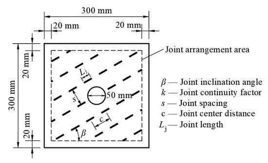
Figure 1.
The dimensions of the specimens and geometrical parameters of the joint set.

Table 1.
Joint geometrical parameters of the tested specimens.
2.2. Specimen Preparation and Test Procedure
The model material used in this study is a mixture of gypsum, Portland cement, and water at a ratio of gypsum: cement: water = 0.99:0.01:0.6 in weight. In addition, a retarder with a dose of 0.05% in weight was added to slow down the setting of the model material. The physical and mechanical properties of the model material are listed in Table 2, which were obtained through the uniaxial compression test, standard triaxial compression test, and Brazilian test.
Table 2.
Physical and mechanical properties of the model material.
Figure 2 shows the mold and fabrication process of a specimen. The mode consists of a cover plate with precut slots and a base plate made of PMMA (polymethyl methacrylate), and a frame and a cylinder made of stainless steel. To make the pre-existing joints, a group of 0.3 mm-thick nickel steel sheets was inserted into the mixture through the precut slots and removed after the start of the liquid mixture solidification. The specimens were cured for 21 days at room temperature. In order to observe repeatable results, the mixing, fabrication, and curing of the material were carefully controlled, and at least two samples with the same joint configuration were prepared for the tests. The mechanical parameters of each series were taken as the average of the two specimens.
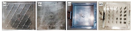
Figure 2.
The mold and fabrication process of a specimen: (a) the cover plate, (b) the base plate, (c) the frame installed with the base plate and the cylinder, and (d) a specimen before solidification.
The uniaxial compression tests were performed in an INSTRON 8506 servo-controlled hydraulic loading system with high stiffness. To obtain complete stress–strain curves, displacement control was applied with a constant loading rate of 0.0025 mm/s. The load and displacement were recorded automatically by the loading system, and fracture propagation on the surface of the specimens were monitored by a digital video and recorded by a high-resolution digital camera.
3. Laboratory Test Results
3.1. Strength and Deformability
Figure 3 shows the laboratory test results for the axial stress–strain curves of the two intact specimens with and without a hole and the jointed specimens with a hole. Chen et al. [] have classified the stress–strain curves of jointed specimens under uniaxial compression into four types according to their different patterns after the first peak, i.e., Type 1—single-peak curve, Type 2—general strain softening with oscillations, Type 3—yield platform-strain softening, and Type 4—yield platform-strain hardening-strain softening. In this study, except for Type 4 deformation behavior, single-peak curve (Type 1) and multi-peak deformation behaviors of Type 2 and 3 were also observed for the jointed specimens with the hole under uniaxial compression. Type 1 deformation behavior was observed for specimens A, HA, HB45, HD45, HB60, HB90, and HC90, Type 2 deformation behavior for specimens HD0, HC30, and HD30, and Type 3 deformation behavior for specimens HB0, HC0, HB30, HC45, HC60, and HD90.
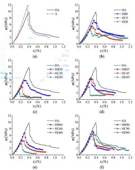
Figure 3.
Axial stress–strain curves of all specimens by laboratory tests. (a) A and HA; (b) β = 0°; (c) β = 30°; (d) β = 45°; (e) β = 60°; (f) β = 90°.
The peak strength σp of specimens A and HA are 11.94 MPa and 10.14 MPa, respectively, and Young’s moduli E (the tangent modulus in the linear elastic stage of an axial stress–strain curve) of the two specimens are 3.84 GPa and 3.02 GPa, respectively. Figure 4 and Figure 5 show the variation of σp and E with the two geometrical parameters, i.e., the joint inclination angle β and the joint continuity factor k. It can be seen that: (1) the peak strength and Young’s modulus of the specimen may decrease significantly in the presence of the hole and the non-persistent open joints; (2) for each value of k, the curves of σp vs. β and E vs. β are W-shaped or V-shaped with the minima and maxima occurring at β = 30° and 90°, respectively; (3) for a constant value of β, the peak strength σp and Young’s modulus E will decrease with increase in the joint continuity factor k, and the fastest and slowest velocity occurs at β = 30°and β = 90°, respectively.
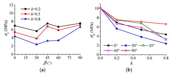
Figure 4.
The peak strength vs. two geometrical parameters of the laboratory tests. (a) σp vs. β; (b) σp vs. k.
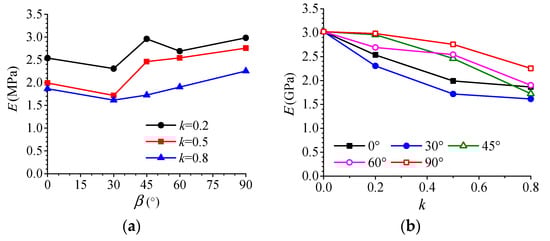
Figure 5.
Young’s modulus vs. two geometrical parameters of the laboratory tests. (a) E vs. β; (b) E vs. k.
3.2. Cracking Process
The anisotropic nonlinear behavior of the jointed specimens with the hole is related to their different cracking process. Figure 6 shows the observed crack initiation types, which are classified according to their mechanism (tensile or shear, represented by T and S, respectively) and position (represented by their lower index), namely, from the matrix (Tm), joint (Tj1, Tj2, and Sj), and periphery of the hole (Th and Sh). Figure 7 shows the observed crack coalescence types between the joints and between the hole and the joint or matrix (initial by H), respectively.
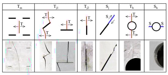
Figure 6.
Observed crack initiation types initiated from the matrix, joints, and hole (Red and blue lines represent tensile or shear cracks, respectively).
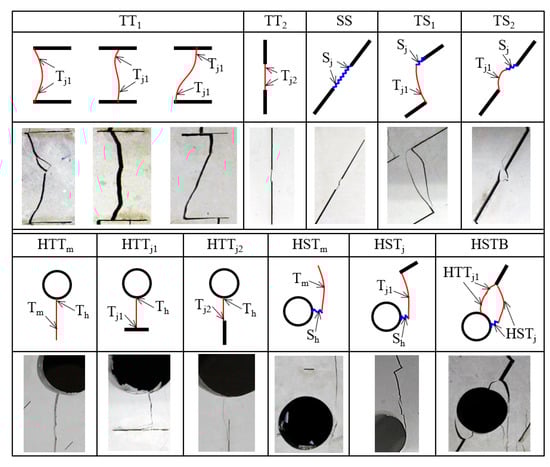
Figure 7.
Observed crack coalescence types between the joints and between the hole and the matrix or joint.
Crack initiation type Tm is produced by an axial tensile crack that emanates from the matrix; crack initiation type Tj1 is produced by a tensile crack or a wing crack that emanates from the tip or middle of the joint, propagates perpendicularly first and then toward the loading direction; crack initiation type Tj2 is a quasi-coplanar tensile crack that emanates from the joint tip, which only occurs in specimens with vertical joints; crack initiation type Sj is a quasi-coplanar shear crack that emanates from the joint tip; crack initiation Th is a tensile crack that emanates from the roof or floor of the hole and propagates toward the loading direction; crack initiation type Sh is a shear crack or crush zone having finite width that emanates from the left or right sides of the hole and propagates perpendicular to the loading direction.
Two types of tensile crack coalescence between the joints were observed, namely, TT1 and TT2, which were formed by the linkage of two type Tj1 tensile cracks and two type Tj2 tensile cracks, respectively. Coalescence Type SS is formed by the linkage of two type Sj shear cracks along the same joint plane. Two types of mixed tensile–shear crack coalescence between the joints were observed, namely, TS1 and TS2, which were formed by the linkage of one Type Tj1 tensile crack and another Type Sj shear crack that started from a different joint plane and the same joint plane, respectively.
Three types of tensile crack coalescence between the hole and the joint or matrix were observed, namely, HTTm, HTTj1, and HTTj2, which were formed by the linkage of a Type Th tensile crack from the hole and a tensile crack of Type Tm from the matrix, or Tj1 and Tj2 from the joint, respectively. Two types of mixed tensile–shear crack coalescence between the hole and the joint or matrix were observed, namely, HSTm and HSTj, which is formed by the linkage of a Type Sh shear crack from the hole and a tensile crack of type Tm or Tj1, respectively. Coalescence type HSJB is produced by the occurrence of the two coalescence types, HSTj and HTTj1, from the same joint, which may cause the formation of a block.
Table 3 summarizes crack coalescence types observed in the jointed specimens with a hole. Tensile crack coalescence between joints of type TT1 and TT2 was found in specimens with horizontal joints or incline joints and those with vertical joints, respectively. Shear cracks coalescence between joints of type SS was found in specimens HD45, HC60, and HD60. Mixed shear–tensile cracks coalescence of type TS1 and TS2 were found in the specimens with inclined joints at medium and larger continuity factors (k = 0.5 and 0.8), i.e., HC30, HD30, HC45, HD45, HC60 and HD60. Tensile cracks coalescence around the hole, i.e., Types HTTm, HTTj1 and HTTj2 were found in all jointed specimens except for specimens HB0 and HB90. Mixed shear–tensile cracks coalescence around the hole of Types HSTm and HSTj were found in all jointed specimens, while coalescence type HSB with formation of blocks was found only in specimens HC45, HD45, and HC60.
Table 3.
Crack coalescence types and collapse modes of the hole observed in the jointed specimens with a hole (Symbols ★ and ▲ represent crack coalescence types between the joints without or with participation of shear crack, respectively; ● and □ represent crack coalescence types between the hole and the joint or matrix without or with participation of shear crack, respectively).
3.3. Collapse Modes of the Hole
Crack coalescence around the hole may lead to a collapse of the hole. Lajtai and Lajtai [] have found that the linkage of the crush zone and secondary tensile cracks in the rock matrix (Coalescence type HSTm) may finally lead to a collapse of the hole in the intact rock samples. The observed collapse modes of the hole can be classified into three types as follows (see Figure 8):
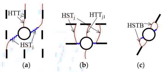
Figure 8.
Observed collapse modes of the hole. (a) Mode Ih; (b) Mode IIh; (c) Mode IIIh.
- (1)
- Mode Ih—without removable blocks, where the linked tensile cracks or shear–tensile cracks around the hole may extend to the boundary of the specimen, and therefore, no removable blocks can be formed;
- (2)
- Mode IIh—with removable blocks formed by upper joints, where the linked tensile cracks or shear–tensile cracks around the hole may extend to the upper joints, leading to the formation of one or several removable blocks;
- (3)
- Mode IIIh—with removable blocks formed by the nearest inclined joints, where coalescence type HSTB may occur from the nearest inclined joints to the hole, leading to the formation of a pair of removable blocks.
The collapse modes of all jointed specimens with a hole are listed in Table 3. Collapse mode IIIh occurs in specimens with coalescence type HSTB, i.e., HC45, HC60, and HD45. Collapse mode II occurs either in specimens with low joint inclination angle (β = 0° and 30°) at the medium or the largest joint continuity factors (k = 0.5 or 0.8), i.e., HD0, HC30, and HD30, or in specimens with the high-joint inclination angles (β = 60° and 90°) at the smallest joint continuity factor (k = 0.2), i.e., HB60 and HB90. Collapse mode I occurs in the other specimens.
Figure 9, Figure 10 and Figure 11 show the cracking process of the specimens with different collapse modes, i.e., specimens HC90, HD0, and HC60. For specimen HC90 of collapse mode Ih (see Figure 9), at the pre-peak stage, Type Tj2 tensile cracks initiated from joints at the right side of the hole first (see Figure 9a), and then Type Th tensile cracks and Type Sh shear cracks initiated from the hole, as well as Type Tj2 wing crack initiated from joints near the left side(see Figure 9b). At the post-peak stage, the linkage of shear cracks at the two sides of the hole with the wing cracks from the joints (coalescence Type HSTj) finally leads to the collapse of the hole (see Figure 9c).
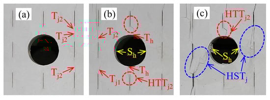
Figure 9.
Cracking process around the hole in specimen HC90 of collapse mode Ih: (a) σ1 = 0.31σp, ε1 = 0.42εp; (b) σ1 = 0.87σp, ε1 = 0.89εp, and (c) σ1 = 0.45σp, ε1 = 1.65εp (Red and blue dotted circles represent crack coalescence types without or with participation of shear crack, respectively).
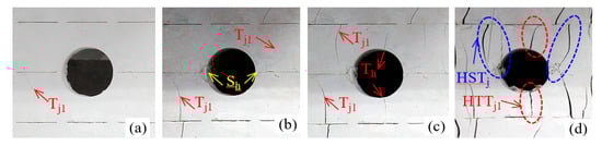
Figure 10.
Cracking process around the hole in specimen HD0 of collapse mode IIh: (a) σ1 = 0.81σp, ε1 = 0.75εp; (b) σ1 = 0.95σp, ε1 = 0.95εp; (c) σ1 = 0.59σp, ε1 = 1.33εp, and (d) σ1 = 0.56σp, ε1 = 3.23εp.
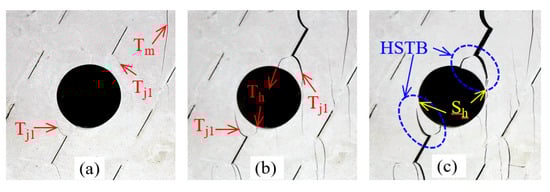
Figure 11.
Cracking process around the hole in specimen HC60 of collapse mode IIIh at: (a) σ1 = 0.96σp, ε1 = 0.96εp; (b) σ1 = 0.85σp, ε1 = 1.13εp, and (c) σ1 = 0.38σp, ε1 = 1.46εp.
For specimen HD0 of collapse mode IIh (see Figure 10), at the pre-peak stage, Type Tj1 tensile cracks initiated from joints at the two sides of the hole first (see Figure 10a), and then Type Sh shear cracks initiated from the two sides of the hole (see Figure 10b). At the post-peak stage, Type Th tensile cracks initiated from the roof and floor of the hole and type Tj1 tensile cracks initiated from the upper joints (see Figure 10c), and the linkage of those cracks (coalescence Types HSTj and HTTj1) led to the formation of the upper removable blocks and, finally, to the collapse of the hole (see Figure 10d).
For specimen HC60 of collapse mode IIIh (see Figure 11), at the pre-peak stage, Type Tj1 wing cracks initiated from the nearest inclined joints, and type Tm tensile cracks initiated in the matrix first (see Figure 11a). At the post-peak stage, Type Th tensile cracks initiated from the upper right and lower left of the hole, and several type Tj1 tensile cracks initiated from other inclined joints around the hole (see Figure 11b). Type Sh shear cracks initiated from the two sides of the hole, and the linkage of these cracks led to the formation of a pair of removable blocks and, finally, to the collapse of the hole (see Figure 11c).
3.4. Failure Modes
Propagation and coalescence of cracks together with the pre-existing joints may cause the formation of continuous fractures, which may finally lead to the failure of the specimen. The observed failure modes in the jointed specimen with a hole can be classified into four types as follows (see Figure 12):
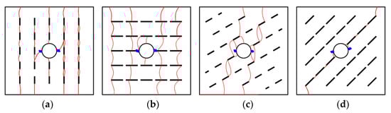
Figure 12.
Failure modes of the jointed specimens with a hole. (a) Mode I—Axial cleavage; (b) Mode II—crushing; (c) Mode III—stepped; (d) Mode IV—sliding.
- (1)
- Mode I—axial cleavage, in which linked vertical tensile fractures may break the specimens into several parts or pillars;
- (2)
- Mode II—crushing, in which linked vertical tensile fractures together with preexisting low inclination angle joints may break the specimens into many small blocks;
- (3)
- Mode III—stepped, in which mixed tensile–shear cracks and the preexisting inclined joints in neighbor columns form one or several stepped failure planes;
- (4)
- Mode IV-sliding, in which quasi-coplanar shear cracks and the preexisting joints form one or several failure planes and lead to sliding along those joint planes.
It should be noted that the four types of failure modes also have been found for jointed specimens without a hole in many pieces of the literature, for example, Prudencio and Jan [] and Chen et.al. [].
Figure 13 presents the failure modes of all jointed specimens with a hole and their fractures. Typical specimens of different failure modes are marked with the red border, i.e., specimens HC90, HD0, HC30, and HD45 with failure modes I to IV, respectively.
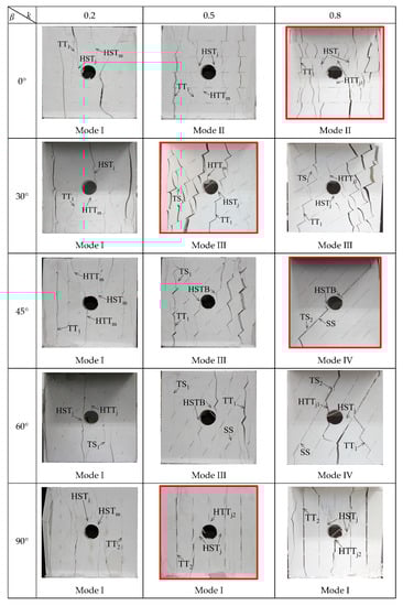
Figure 13.
Fractures of all jointed specimens with a hole and their failure modes (the typical specimens with different failure modes are marked with the red border).
Failure mode I occurs in specimens at the smallest joint continuity factor (k = 0.2) or with vertical joints (β = 90°), namely, specimens HB0, HB30, HB45, HB60, HB90, HC90, and HD90. Failure mode II occurs in specimens with horizontal joints (β = 0°) at medium and the largest joint factors (k = 0.5 and 0.8), namely, specimens HC0 and HD0. Failure mode III occurs in specimens with inclined joints (β = 30°, 45°, and 60°) at medium joint factor (k = 0.5) or specimens with β = 30° at the largest joint factor (k = 0.8), namely, specimens HC30, HC45, HC60, and HD30. Failure mode IV occurs in specimens with β = 45° and 60° at the largest joint factor (k = 0.8), namely, specimens HD45 and HD60. In general, specimens with failure modes III or IV that are characterized by involving shear crack propagation may have lower peak strength than those with failure modes I and II.
4. FE Analysis Based on the MPD Model
4.1. A brief Introduction to the MPD Model for Rocks
Figure 14 shows the flowchart of the MPD model for rocks in a VUMAT user subroutine of ABAQUS. For a representative volume element (RVE) of a rock or a rock mass, a kinematic constraint is assumed for correlations between macroscopic and microplane stress/strain. Namely, the microplane strain vector of the rock mass is the directional projection of the macroscopic strain tensor , while the macroscopic stress tensor can be obtained by the directional integral of all microplane stress vectors of the rock mass , according to the principle of variational work, which can be given by the following:
where and are tensorial components of the macroscopic stress and strain tensor, respectively, where the subscripts i, j = 1, 2, 3 refer to the global Cartesian coordinate ; , , and are the unit normal vector of the microplane and the two orthogonal unit vectors on the microplane; , and are the normal and the two shear components of microplane stress and strain vectors; is the integral over the surface of a unit sphere, where and are the spherical angles. Here, Einstein summation convention is adopted, i.e., repetition of subscripts implies summation over 1, 2, and 3.
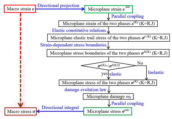
Figure 14.
Flowchart of the MPD model for rocks in a VUMAT user subroutine of ABAQUS.
A microplane of the rock mass can be seen as a combination of the two phases, namely, the rock matrix and the rock joint. The ratio of the joint phase on the microplane is selected as the damage variable. On each microplane, the two phases are mechanically coupled in parallel; namely, the microplane strain vector of each phase is identical to that of the rock mass , while the microplane stress vector of the rock mass is the summation of that of the two phases weighted by their ratios:
On the microplane, the elastic behavior of the two phases can be described by their linear elastic laws. The inelastic behavior of the two phases on the microplane under tension, compression, and shear loading can be described by their corresponding strain-dependent stress boundaries. The details of the linear elastic laws and strain-dependent stress boundaries of the two phases can be found in Chen and Bažant []. For each phase, the elastic trail stress will be returned to the stress boundaries if it exceeds the boundary.
To reflect the initiation and propagation of tensile or shear cracks due to the accumulation of volumetric expansion, normal extension, or shear deformation on microplanes, the microplane damage evolution law was given by the power law of the historic strains as follows:
where are the maximum volumetric expansion strain, deviatoric tensile strain, and shear strain reached so far on the microplane, respectively; a1, a2, a3, q1, q2, and q3 material constants control damage evolution related to .
To measure the overall damage of the RVE, the directional average of for all microplanes, namely, damage ω0, was also calculated and can be given by the following:
where is the number of the numerical integration points on a unit hemisphere surface, is the weight of the m-th microplane, and is the damage variable on the m-th microplane.
The value of the microplane damage and the average damage ω0 are always between 0 and 1. For a microplane, and represent no crack/joint and a continuous crack/joint on the microplane, respectively. For the RVE, and represent no damage (the intact RVE without any crack/joint) and entire damage (the RVE full of joint material), respectively.
4.2. FE Model and Calibration of the Material Parameters
The size of the numerical model is the same as that in the physical experiment. Figure 15 shows the FE model of specimen HC45 (κ = 0.5 and β = 45°). The top and bottom loading plates are rigid bodies, loaded at a constant displacement rate and fixed, respectively. The pre-existing joints are modeled by a rectangle opening with a thickness of 0.3 mm. The element type used here is a six-node linear triangular prism (C3D6), and the total number of elements is about 200,000.
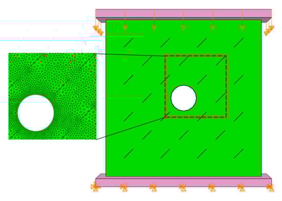
Figure 15.
The FE model of specimen HC45 and the location of the five selected elements.
The twenty material parameters of the MPD model used in numerical modeling are calibrated by specimens A and HA (the intact specimens with or without a hole) and are listed in Table 4. The calibration method for these parameters can be given as follows: (1) Young’s modulus and Poisson’s ratio of the rock matrix, and , can be obtained from Table 2. The same values were taken for those of the rock joint or crack and for simplicity; (2) parameters ε0V, ε0N, c1, c2, c3, c4, a1, a2, a3 q1, q2, and q3 mainly control the shape of the nonlinear stress–strain curve and can be set as the similar values for a certain type of rocks; (3) parameters T(R), T(J), α0, and βc can be obtained from optimal fitting to the stress–strain curves of the specimens.
Table 4.
Material parameters of the MPD model used in numerical modeling.
4.3. Numerical Results of Macroscopic Mechanical Response
Figure 16 shows the axial stress–strain curves of specimens A and HA (the intact specimens with or without a hole, respectively) as well as all the jointed specimens with a hole obtained by numerical simulation. Figure 17 and Figure 18 show curves of the peak strength and Young’s modulus vs. the two geometrical parameters by numerical simulation.
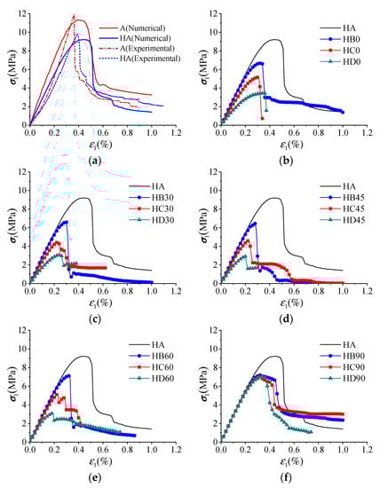
Figure 16.
Axial stress–strain curves of all specimens by numerical simulation. (a) A and HA; (b) β = 0°; (c) β = 30°; (d) β = 45°; (e) β = 60°; (f) β = 90°.
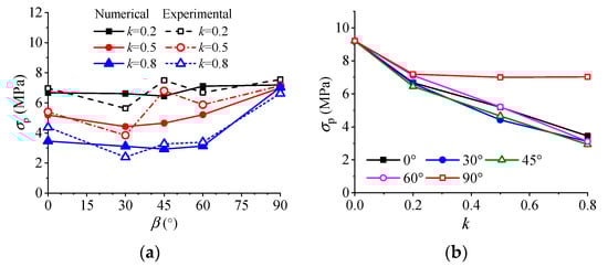
Figure 17.
The peak strength vs. the two geometrical parameters by numerical simulation. (a) σp vs. β; (b) σp vs. k.
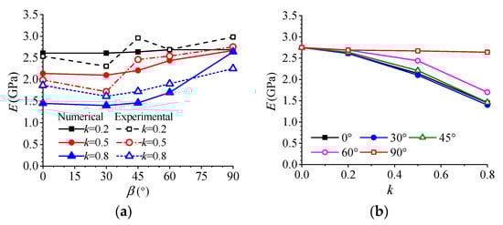
Figure 18.
Young’s modulus vs. the two geometrical parameters by numerical simulation. (a) E vs. β; (b) E vs. k.
In Figure 16a, Figure 17a and Figure 18a, results by laboratory tests were also depicted for comparison. In general, the numerical results can reproduce the main features observed in laboratory tests, including dependence of the deformation behavior, peak strength, and Young’s modulus on the joint inclination angle β and the joint continuity factor k.
4.4. Failure Mechanism of the Intact Specimen with the Hole
The nonlinear mechanical response of specimen HA under uniaxial compression can be related to stress concentration and damage evolution in the matrix around the hole. The problem of the disturbance of the elastic stress field caused by the presence of the hole under far-field uniaxial compression was solved by Kirsch in 1898. Accordingly, the radial and hoop stress concentration factor (σr/σ1) and (σθ/σ1) can be given as follows (see the textbook of Jaeger et al. []):
where r is the distance to the hole center; a is the radius of the circular hole; θ is the angle of rotation from the axial stress σ1; σr and σθ are the radial and hoop stresses in the specimen.
The maximum tensile and compressive stress may occur along the hole periphery, with at θ = 0° or 180° (the roof or floor) and at θ = 90° or 270° (the right or left side), respectively.
Figure 19a,b shows hoop stress σθ in specimen HA at the early elastic deformation stage, when σ1 = 1 MPa and the peak strength, when σ1 = σp, respectively. Figure 19c,d shows damage ω0 at σ1 = σp and fractures observed in the experiment. Figure 20 and Figure 21 show the variation of radial and hoop stress concentration factors (σr/σ1) and (σθ/σ1) and the average damage of all microplanes ω0 vs. distance ratio r/a along a horizontal or vertical plane in specimen HA at σ1 = 1 MPa and σ1 = σp, respectively.
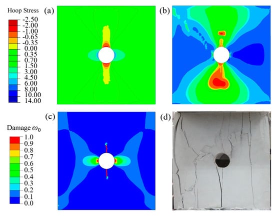
Figure 19.
Hoop stress σθ and damage ω0 in specimen HA: (a) σθ at σ1 = 1 MPa, (b) σθ at σ1 = σp, (c) ω0 at σ1 = σp, and (d) fractures observed in the experiment.
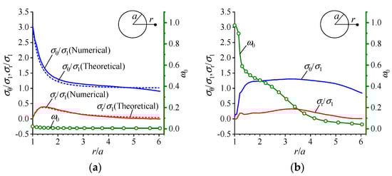
Figure 20.
σr/σ1, σθ/σ1, and ω0 vs. r/a along horizontal plane in specimen HA. (a) σ1 = 1 MPa; (b) σ1 = σp.
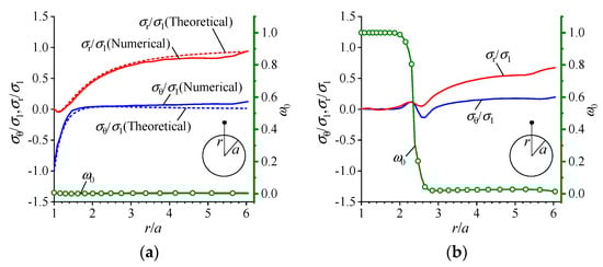
Figure 21.
σr/σ1, σθ/σ1, and ω0 vs. r/a vs. distance ratio r/a along vertical plane in specimen HA. (a) σ1 = 1 MPa; (b) σ1 = σp.
At the early elastic deformation stage, when σ1 = 1 MPa, tensile or compressive stress concentrate at the roof/floor and the left/right sides of the hole periphery (see Figure 19a), respectively. The results of (σr/σ1) and (σθ/σ1) vs. r/a by numerical simulation are very close to those by theoretical solution for the elastic solid since damage ω0 remains almost zero when σ1 = 1 MPa (see Figure 20a and Figure 21a).
At the peak strength, when σ1 = σp, damage evolution due to tensile or compressive stress concentration is localized in two narrow vertical bands above or below the hole or in two small horizontal zones at the two sides of the hole (see Figure 19c), respectively. As shown in Figure 20b and Figure 21b, the length of the vertical damage bands and the horizontal damage zones are about 1.5a and 0.5a, respectively. Due to stress loosening in damage localization zones, the current tensile or compressive stress concentration areas will move to the front of the damage zones (see Figure 19b). In general, fractures in specimen HA coincide very well with the damage localization areas.
4.5. Failure Mechanism of the Jointed Specimens with the Hole
The nonlinear mechanical response of the jointed specimens with the hole under uniaxial compression may be much different from that of the intact specimen with the hole since the presence of the joints may influence stress concentration, damage evolution, and inelastic deformation development.
4.5.1. Influence of Joints on Stress Concentration at Elastic Stage
For a single elliptic crack in an infinite elastic solid subject to a far-field uniaxial compression stress σ1, the stress concentration around the crack has been solved by Muskhelishvili in 1963 and can be found in the textbook of Jaeger et al. []. Lajtai [] discussed the influence of the axial ratio b/a (the ratio of the smaller to the larger semiaxis) and the inclination angle β on the stress concentrations along an elliptic crack periphery, and the extent and shape of tensile zone beyond the periphery of a flat crack (b/a = 0).
In this study, the length of the joints in specimen groups HB, HC, and HD is 10, 25, and 40 mm, respectively, while the joint aperture is fixed at 0.3 mm for all specimen groups, and the axial ratio b/a of the equivalent elliptic crack is 0.03, 0.012, and 0.075, respectively. The minimum and maximum principal stress concentration factors σmin/σ1 and σmax/σ1 around the elliptic crack have been calculated for b/a = 0.03 and β = 0°, 45°, and 90° and are plotted in Figure 22.
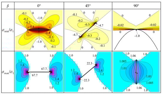
Figure 22.
The distribution of σmin/σ1 and σmax/σ1 around an elliptic crack with the axial ratio b/a = 0.03 and β = 0°, 45° and 90° in an infinite elastic solid subject to a far-field uniaxial compression stress σ1.
For β = 0° and 45°, the elliptic crack produces large tension zones around the whole crack periphery with σmin/σ1 = −1 and near the two ends with σmin/σ1= −4.7, respectively; it induces small zones of very high compressive stress concentration around the crack tips, with σmax/σ1 = 67.7 and 22.3, respectively. For β = 90°, the elliptic crack produces very small tensile zones at the crack tips with σmin/σ1 = −1 and nearly no compressive stress concentration around the crack periphery with σmax/σ1 = 1~1.06. With the decrease in the axial ratio b/a, the magnitude of the maximum tension for the inclined elliptic crack and the order of magnitude of the maximum compression for the inclined and horizontal elliptic crack will increase. The stress concentration around the elliptic crack can explain the crack initiation around the joints, including tensile crack initiation from the middle of the horizontal joints and wing crack initiation from the inclined joints, and shear crack initiation from the tips of the inclined joints (see Figure 6).
For the specimens with the hole and multiple joints, stress concentration around the hole and the joints will be affected by their interaction. At the early elastic stage when σ1 = 1 MPa, Figure 23 and Figure 24 show the distribution of hoop stress σθ and hoop stress concentration factor (σθ/σ1) along the hole periphery in the specimens with k = 0.2 and 0.8 at β = 0°, 45°, and 90°, respectively.
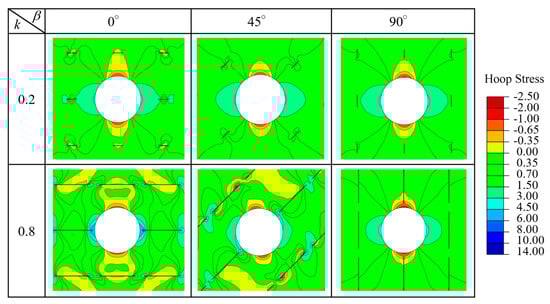
Figure 23.
Hoop stress distribution at σ1 = 1 MPa in specimens with k = 0.2 and 0.8 at β = 0°, 45° and 90°.
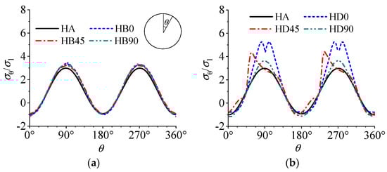
Figure 24.
σθ/σ1 along the hole periphery at σ1 = 1 MPa in the specimens with k = 0.2 and 0.8 at β = 0°, 45° and 90°. (a) k = 0.2; (b) k = 0.8.
When the joint continuity factor is the smallest, i.e., k = 0.2, either the interaction among the small joints or the interaction between the joints and the hole is not obvious. The joints in these specimens only produce stress concentration in the small areas around themselves; therefore, the joint orientation may have little influence on the stress distribution in the other area of the specimen. For all values of β, the values of (σθ/σ1)min are between (−0.94~ −1.18) and occur at θ = 0° (the roof) or 180° (the floor), while the values of (σθ/σ1)max are between (3.23~3.51) and occur at θ = 90° (the right side) or 270° (the left side). When the joint continuity factor is the largest, i.e., k = 0.8, the interaction among the large joints and the interaction between the joints and the hole may become significant, except for the vertical joints. For specimen HD90 (k = 0.8 and β = 90°), tensile stress concentration increases slightly in the presence of the nearest vertical joints near the top and the bottom, while compressive stress concentration changes a little, with (σθ/σ1)min = −1.18 and (σθ/σ1)max = 3.64 occurring at the roof/floor and the two sides of the hole, respectively. For specimen HD0 (k = 0.8 and β = 0°), a small decrease in tensile stress concentration and a significant increase in compressive stress concentration due to adjacent horizontal joints were found, with (σθ/σ1) min = −0.78 at the roof/floor and (σθ/σ1)max= 5.29 at the two sides, respectively. For specimen HD45 (k = 0.8 and β = 45°), nearly no changes in tensile stress concentration and a salient increase in compressive stress concentration were found, with (σθ/σ1)min = −1.04 at θ = 346.4° or 166.4° nearby the roof/floor and (σθ/σ1)max= 4.42 at θ = 58.7°or 234.2° close to the nearest inclined joints, respectively. In general, the nearest joints, which are located on the intersecting joint plane to the hole, may have a significant influence on the stress concentration around the hole.
4.5.2. Influence of Joints on Damage Evolution and Stress Loosening
At peak strength, when σ1 = σP, Figure 25 and Figure 26 show the distribution of hoop stress σθ and damage ω0 in the specimens, with k = 0.2 and 0.8 at β = 0°, 45°, and 90°, respectively.
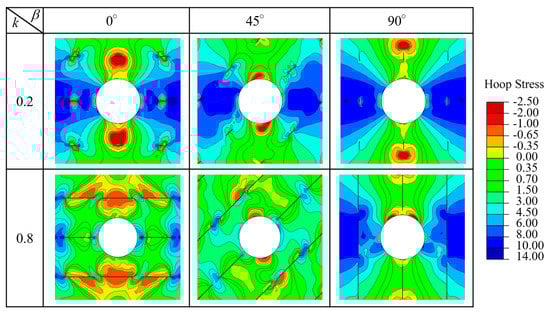
Figure 25.
Hoop stress distribution at σ1 = σp in the specimens with k = 0.2 and 0.8 at β = 0°, 45°, and 90°.
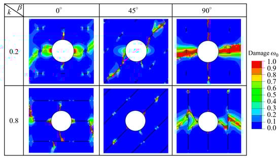
Figure 26.
Damage distribution at σ1 = σp in the specimens with k = 0.2 and 0.8 at β = 0°, 45°, and 90°.
Similar to the intact specimen containing the hole (specimen HA), damage developed from the initial tensile or compressive stress concentration areas and propagated into localization zones, which could lead to stress loosening in these zones and transfer of the current stress concentration areas from the hole neighborhood to the interior.
Even for the specimens with the smallest joint continuity factor (k = 0.2), joint orientation has a salient influence on damage localization and stress concentration. For specimens with horizontal or vertical joints, i.e., HB0, HD0, HB90, and HD90, narrow vertical tensile damage localization bands and wide compressive horizontal damage localization zones developed from the roof/floor and the two sides of the hole, respectively. For specimens with inclined joints, i.e., HB45 and HD45, the current tensile stress concentration areas still located near the roof and floor since no damage developed in these areas; oblique compressive damage localization zones developed from the two sides (for specimen HB45) or the upper left/lower right sides (for specimen HD45) of the hole linked with coplanar damage zones in the rock bridges along the intersecting joint plane to form a failure plane. With the increase in joint continuity factor, widths of compressive damage localization zones and the length of tensile damage bands around the hole may decrease due to the decrease in the rock bridge length.
Figure 27 shows the evolution of hoop stress and damage of elements 1 (σθ1 and ω01) and 2 (σθ2 and ω02) in the specimens with k = 0.2 and 0.8 at β = 0°, 45°, and 90°, respectively. For each specimen, tensile and compressive strain softening happens in elements 1 (at the top) and 2 (at the right side), respectively. Due to the high compressive stress concentration, damage in element 2 grows earlier and faster than damage in element 1 (except for specimen HD90, due to the influence of the adjacent vertical joints); the peak stress in the two elements occurs much earlier than the peak strength of the specimen (except for specimen HD45).
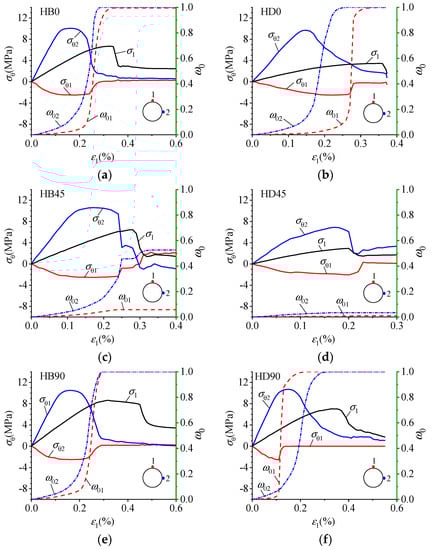
Figure 27.
Evolution of σθ1, σθ2, ω01, and ω02 in the specimens with k = 0.2 and 0.8 at β = 0°, 45°, and 90°: (a) HB0 (k = 0.2 and β = 0°); (b) HD0 (k = 0.8 and β = 0°); (c) HB45 (k = 0.2 and β = 45°); (d) HD45 (k = 0.8 and β = 45°); (e) HB90 (k = 0.2 and β = 90°); (f) HD90 (k = 0.8 and β = 90°).
For specimens with horizontal or vertical joints, i.e., HB0, HD0, HB90, and HD90, due to stress concentration in the two elements at the early elastic stage, damages ω01 and ω02 grow rapidly and reach the maximum value 1 (represent entire damage on all microplanes) before the peak strength leads to strain softening and stress loosening of the two elements (see Figure 27a,b,e,f). For specimens with inclined joints, i.e., HB45 and HD45, damage ω02 grows slowly during the whole loading process (damage starts from element 2 firstly and then propagates toward the nearest inclined joint, see Figure 26), leading to partial stress loosening of the two elements at peak strength. For specimen HD45, due to the deflection of stress concentration areas at the early elastic stage, the average damage ω0 of the two elements grows slowly and is not large (in specimen HB45) or very small (in specimen HD45) during the whole loading process, leading to partial or no stress loosening of these elements at peak strength. Figure 28 shows the variation of the hoop stress concentration factor of elements 1 (σθ1/σ1) and 2 (σθ2/σ1) with joint inclination angle β at peak strength σ1 = σP for all jointed specimens with the hole. For each joint continuity factor, curves of σθ1 /σ1 vs. β and σθ2/σ1 vs. β are anti-V or U, or M shaped with the maxima at β = 30° or 45°, or 60° and the minima at β = 0° or 90°. The hoop stress concentration factor of the two elements σθ1 /σ1 and σθ2/σ1 increases with the increase in the joint continuity factor k. It seems that the hoop stress concentration factor at peak strength can be related to the strength of the specimen; namely, a higher hoop stress concentration factor at σ1 = σP corresponds to a lower strength.
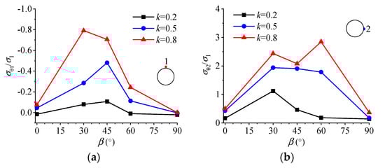
Figure 28.
σθ1 /σ1 and σθ2/σ1 vs. joint inclination angle β at σ1 = σp. (a) σθ1 /σ1; (b) σθ2 /σ1.
Figure 29 shows damage ω0 and displacement vector at the final step in the four typical specimens with different failure modes, i.e., specimens HC90, HD0, HC30, and HD45. In general, the damage localization zones by numerical simulation coincide with the fractures observed in the experiment (see Figure 13) very well. The distribution of the displacement vector in specimen HC30 reveals the departure movement along the stepped failure plane, and that in specimen HD 45 reveals a sliding of the upper block along the diagonal failure plane.
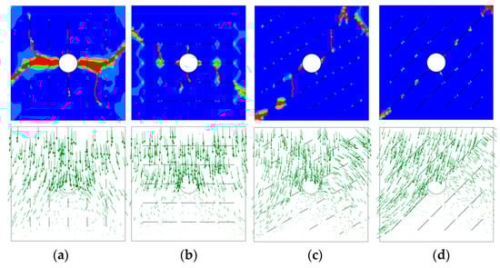
Figure 29.
Damage ω0 and displacement vector at the final step in the four typical specimens with different failure modes. (a) HC90 (Mode I); (b) HD0 (Mode II); (c) HC30 (Mode III); (d) HD45 (Mode IV).
Figure 30 shows the displacement vector around the hole at the final step in the three typical specimens with different collapse modes, i.e., specimens HC90, HD0, and HC60. The opposite horizontal displacement component at the roof in specimen HC90 or floor in specimen HD0 implies normal departure movement along the tensile damage zones. Compressive shear movement occurs in damage zones at the two sides of the hole in specimens HC90 and HD0 or in the areas between the hole surface and the nearest inclined joints in specimen HC60. The blocks moving into the hole marked by the rectangle areas agree with those observed in the laboratory test.
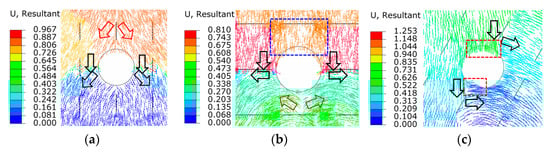
Figure 30.
Displacement vector around the hole at the final step in the three typical specimens of different collapse modes (The unit is mm, and the removable blocks are marked by the rectangle areas). (a) HC90 (Mode Ih); (b) HD0 (Mode IIh); (c) HC60 (Mode IIIh).
5. Conclusions
In this study, the combined influence of joint persistence and orientation on the mechanical behavior of a jointed rock mass with a hole under uniaxial compression has been investigated by physical modeling and FE analysis based on a microplane damage model for rocks.
The peak strength σp and Young’s modulus E may decrease with the increase in joint continuity factor k, and variation of σp and E with joint inclination angle β are the W-shaped or V-shaped curves with the minima and maxima occurring at β = 30° and 90°, respectively. Compared with specimens of failure mode I-axial cleavage or II-crushing, specimens of the failure mode III-stepped or IV-sliding may have a lower peak strength due to involving of shear crack coalescence and sliding failure, which occurs in specimens with inclined joints (β = 30°, 45°, and 60°) at the medium or the largest joint continuity factor (k = 0.5 or 0.8). For most of the specimens, both tensile cracks and crush zones may initiate at the roof/floor and the left/right sides of the hole, respectively, and their linkage with tensile or shear cracks starting from the joints or matrix may lead to the collapse of the hole by three different modes, namely, Mode Ih—without removable blocks, Mode IIh—with removable blocks formed by the upper joints, and Mode IIIh—with removable blocks formed by the nearest inclined joints.
The numerical simulation can not only reproduce the main features of macroscopic mechanical behavior observed in physical modeling but also explain the failure process, such as stress concentration, damage evolution, and stress loosening, as well as the interaction mechanisms between the hole and the joints. The strong interaction between the hole and the nearest joints was revealed. At the elastic stage, stress concentration around the hole will be altered by the presence of the joints, and the effect may be strengthened with the increase in the joint continuity factor k. Vertical joints (β = 90°) will have the least influence on stress concentration around the hole, horizontal joints (β = 0°) will induce the largest compressive stress concentration at the two sides of the hole, and inclined joints (β = 30°, 45 and 60°) may cause salient deflection of compressive stress concentration areas around the hole. At the peak strength, stress loosening may happen much earlier before peak strength due to the damage evolution, and the current stress concentration areas will be transferred from the hole surface to the interior. Hoop stress concentration around the hole can be related to the strength of the specimen, i.e., a higher hoop stress concentration factor may lead to lower strength.
Author Contributions
Conceptualization, X.C.; methodology, X.C.; software, X.L.; validation, X.L.; investigation, R.L.; data curation, Z.F.; writing—original draft preparation, X.C.; writing—review and editing, X.C. All authors have read and agreed to the published version of the manuscript.
Funding
This research work was financially supported by the National Natural Science Foundation of China (No. 41941018 and 11572344) and the National Key Research and Development Program of China (No. 2019YFC1521000).
Data Availability Statement
Not applicable.
Conflicts of Interest
The authors declare that they have no known competing financial interest or personal relationships that could have appeared to influence the work reported in this paper.
References
- Martini, C.D.; Read, R.S.; Martino, J.B. Observations of brittle failure around a circular test tunnel. Int. J. Rock Mech. Min. Sci. 1997, 34, 1065–1073. [Google Scholar] [CrossRef]
- Martino, J.B.; Chandler, N.A. Excavation-induced damage studies at the Underground Research Laboratory. Int. J. Rock Mech. Min. Sci. 2004, 41, 1413–1426. [Google Scholar] [CrossRef]
- Thury, M.; Bossart, P. The Mont Terri rock laboratory, a new international research project in a Mesozoic shale formation, in Switzerland. Eng. Geol. 1999, 52, 347–359. [Google Scholar] [CrossRef]
- Li, S.J.; Yu, H.; Liu, Y.X.; Wu, F.J. Results from in-situ monitoring of displacement, bolt load, and disturbed zone of a powerhouse cavern during excavation process. Int. J. Rock Mech. Min. Sci. 2008, 45, 1519–1525. [Google Scholar] [CrossRef]
- Germanovich, L.N.; Dyskin, A.V. Fracture mechanisms and instability of openings in compression. Int. J. Rock Mech. Min. Sci. 2000, 37, 263–284. [Google Scholar] [CrossRef]
- Lee, C.; Wang, S.J.; Yang, Z.F. Geotechnical aspects of rock tunnelling in China. Tunn. Undergr. Space Technol. 1996, 11, 445–454. [Google Scholar] [CrossRef]
- He, M.C.; Gong, W.L.; Zhai, H.M.; Zhang, H.P. Physical modeling of deep ground excavation in geologically horizontal strata based on infrared thermography. Tunn. Undergr. Space Technol. 2010, 25, 366–376. [Google Scholar] [CrossRef]
- Huang, F.; Zhu, H.; Xu, Q.; Cai, Y.; Zhuang, X. The effect of weak interlayer on the failure pattern of rock mass around tunnel—Scaled model tests and numerical analysis. Tunn. Undergr. Space Technol. 2013, 35, 207–217. [Google Scholar] [CrossRef]
- Lajtai, E.Z.; Lajtai, V.N. The collapse of cavities. Int. J. Rock Mech. Min. Sci. 1975, 12, 81–86. [Google Scholar] [CrossRef]
- Wong, R.; Lin, P.; Tang, C.; Chau, K. Creeping damage around an opening in rock-like material containing non-persistent joints. Eng. Fract. Mech. 2002, 69, 2015–2027. [Google Scholar] [CrossRef]
- Sagong, M.; Park, D.; Yoo, J.; Lee, J.S. Experimental and numerical analyses of an opening in a jointed rock mass under biaxial compression. Int. J. Rock Mech. Min. Sci. 2011, 48, 1055–1067. [Google Scholar] [CrossRef]
- Yang, S.Q.; Yin, P.F.; Zhang, Y.C.; Chen, M.; Zhou, X.P.; Jing, H.W.; Zhang, Q.Y. Failure behavior and crack evolution mechanism of a non-persistent jointed rock mass containing a circular hole. Int. J. Rock Mech. Min. Sci. 2019, 114, 101–121. [Google Scholar] [CrossRef]
- Kawamoto, T.; Ichikawa, Y.; Kyoya, T. Deformation and fracturing behaviour of discontinuous rock mass and damage mechanics theory. Int. J. Numer. Anal. Methods Geomech. 1988, 12, 1–30. [Google Scholar] [CrossRef]
- Swoboda, G.; Shen, X.P.; Rosas, L. Damage model for jointed rock mass and its application to tunnelling. Comput. Geotech. 1998, 22, 183–203. [Google Scholar] [CrossRef]
- Yeung, M.R.; Leong, L.L. Effects of joint attributes on tunnel stability. Int. J. Rock Mech. Min. Sci. 1997, 34, 348.e1–348.e18. [Google Scholar] [CrossRef]
- Einstein, H.H.; Veneziano, D.; Baecher, G.B.; O”Reilly, K.J. The effect of discontinuity persistence on rock slope stability. Int. J. Rock Mech. Min. Sci. 1983, 20, 227–236. [Google Scholar] [CrossRef]
- Lajtai, E.Z. Strength of discontinuous rock in direct shear. Geotechnique 1963, 19, 218–233. [Google Scholar] [CrossRef]
- Chen, X.; Liao, Z.H.; Li, D.J. Experimental study on the effect of joint orientation and persistence on the strength and deformation properties of rock masses under uniaxial compression. Chin. J. Rock Mech. Eng. 2010, 30, 781–789. [Google Scholar]
- Chen, X.; Liao, Z.; Xi, P. Deformability characteristics of jointed rock masses under uniaxial compression. Int. J. Min. Sci. Technol. 2012, 22, 213–221. [Google Scholar] [CrossRef]
- Su, H.; Zhang, H.; Qi, G.; Lu, W.; Wang, M. Preparation and CO2 adsorption properties of TEPA-functionalized multi-level porous particles based on solid waste. Colloids Surf. A Physicochem. Eng. Asp. 2022, 653, 130004. [Google Scholar] [CrossRef]
- Han, W.; Jiang, Y.; Luan, H.; Du, Y.; Zhu, Y.; Liu, J. Numerical investigation on the shear behavior of rock-like materials containing fissure-holes with FEM-CZM method. Comput. Geotech. 2020, 125, 103670. [Google Scholar] [CrossRef]
- Bažant, Z.P. Microplane Model for Strain-Controlled Inelastic Behavior; Chapter 3, Mechanics of engineering materials; Desai, C.S., Gallagher, R.H., Eds.; Wiley: London, UK, 1984. [Google Scholar]
- Bažant, Z.P.; Oh, B.H. Microplane model for progressive fracture of concrete and rock. J. Eng. Mech. 1985, 111, 559–582. [Google Scholar] [CrossRef]
- Bažant, Z.P.; Caner, F.C.; Carol, I.; Adley, M.D.; Akers, S.A. Microplane model M4 for concrete. I: Formulation with work-conjugate deviatoric stress. J. Eng. Mech. 2000, 126, 944–953. [Google Scholar] [CrossRef]
- Caner, F.; Bažant, Z. Microplane model M7 for plain concrete: I. Formulation. J. Eng. Mech. 2013, 139, 1714–1735. [Google Scholar] [CrossRef]
- Bažant, Z.P.; Prat, P.C. Creep of Anisotropic Clay: Microplane Model. J. Geotech. Eng. 1986, 112, 458–475. [Google Scholar] [CrossRef]
- Prat, P.C.; Bažant, Z.P. Microplane model for triaxial deformation of saturated cohesive soils. Int. J. Rock Mech. Min. Sci. 1992, 117, 891–912. [Google Scholar] [CrossRef]
- Bažant, Z.P.; Zi, G. Microplane constitutive model for porous isotropic rocks. Int. J. Numer. Anal. Methods Geomech. 2003, 27, 25–47. [Google Scholar] [CrossRef]
- Chen, X.; Bažant, Z.P. Microplane damage model for jointed rock masses. Int. J. Numer. Anal. Methods Geomech. 2014, 38, 1431–1452. [Google Scholar] [CrossRef]
- Gowd, T.N.; Rummel, F. Effect of confining pressure on the fracture behaviour of a porous rock. Int. J. Rock Mech. Min. Sci. 1980, 17, 225–229. [Google Scholar] [CrossRef]
- Chen, X.; Fu, Y.; Feng, Z.L. Microplane Damage Model for Rocks and Its Application. In Proceedings of the 14th International Congress on Rock Mechanics and Rock Engineering, Foz do Iguassu, Brazil, 13–18 September 2019; pp. 2984–2992. [Google Scholar]
- Prudencio, M.; Jan, M.V.S. Strength and failure modes of rock Mass models with non-persistent joints. Int. J. Rock Mech. Min. Sci. 2007, 44, 890–902. [Google Scholar] [CrossRef]
- Chen, X.; Liao, Z.H.; Peng, X. Cracking process of rock mass models under uniaxial compression. J. Cent. South Univ. 2013, 20, 1661–1678. [Google Scholar] [CrossRef]
- Jaeger, J.C.; Cook, N.G.W.; Zimmerman, R.W. Fundamentals of Rock Mechanics, 4th ed.; Blackwell: Hoboken, NJ, USA, 2007; p. 218. [Google Scholar]
- Lajtai, E.Z. A theoretical and experimental evaluation of the Griffith theory of brittle fracture. Tectonophysics 1971, 11, 129–156. [Google Scholar] [CrossRef]
Disclaimer/Publisher’s Note: The statements, opinions and data contained in all publications are solely those of the individual author(s) and contributor(s) and not of MDPI and/or the editor(s). MDPI and/or the editor(s) disclaim responsibility for any injury to people or property resulting from any ideas, methods, instructions or products referred to in the content. |
© 2023 by the authors. Licensee MDPI, Basel, Switzerland. This article is an open access article distributed under the terms and conditions of the Creative Commons Attribution (CC BY) license (https://creativecommons.org/licenses/by/4.0/).