Advanced Control Algorithm for Three-Phase Shunt Active Power Filter Using Sliding DFT

Abstract

This paper describes n digital control algorithm for a three-phase shunt active power filter (APF) using switching–sliding discrete Fourier transform (SSDFT). Traditionally, APF control algorithms use first harmonic detector circuits, which can be implemented using the SDFT algorithm. The classical SDFT algorithm is characterized by long-term stability issues, resulting from numerical errors. Many complex modifications to improve the stability of the SDFT algorithm have been proposed in the scientific literature. This article proposes a solution to the SDFT stability problem using the basic structure of the algorithm. The authors propose the use of the switching SDFT algorithm, where two original SDFT algorithms are implemented in parallel. Both algorithms are turned on alternately after a set period of time and reset to zero in order to reset numerical errors causing their unstable operation. Compared to the classical three-phase SDFT algorithm, the three-phase SSDFT requires only about 25% more arithmetic operations. The proposed approach has been validated using experimental tests and dramatically reduces the numerical errors. The control algorithm has been implemented using the TMS320F28379D microcontroller. The sampling method using only the internal A/D converter of a microcontroller is also presented. The article includes the experimental test results of the complete APF.

1. Introduction

In the initial period of power engineering development, at the end of the nineteenth century, DC power was developed, which, however, was relatively quickly replaced by AC power. This led to the idea of three-phase circuits, which were pioneered by a Polish engineer, Michał Doliwo-Dobrowolski [1,2,3], among others. During the International Electrotechnical Exhibition in Frankfurt am Main, Germany, in 1891, AEG presented the first remote three-phase high voltage (15 kV) transmission line for electrical energy with a length of about 175 km, based on the concept of the AEG main constructor Michał Doliwo-Dobrowolski. In the same year, he also created a three-phase transformer and short-circuited (squirrel-cage) three-phase induction motor.

It is also worth noting that one of the world’s first three-phase high voltage (10 kV) transmission lines for electrical energy was launched in 1896 in the area of the current Lubuskie Voivodeship, Poland. This line, 25 km long, connected the hydroelectric plant on the Bóbr River in Nowogród Bobrzański with the city of Zielona Góra [1,4].

To this day, electrical energy is transmitted chiefly using three-phase lines. In power stations, three-phase sinusoidal voltage is mainly produced by synchronous generators. It is vital to ensure that the output voltage closely follows the shape of an ideal sinusoidal waveform and that it is symmetrical in all phases. In the initial phases of development, the typical loads, such as light bulbs and electrical heaters, were linear loads, ensuring that the voltage and current in transmission lines remained sinusoidal. The increasing use of such devices as arc furnaces, saturated transformers, and semiconductor switches draws non-sinusoidal currents from the power line. With further development of power electronics, the share of nonlinear receivers began to grow rapidly, and now more than 80% of electricity is converted by power electronics circuits.

As a result of this, non-sinusoidal currents and voltages appear within transmission lines and transformers. As a direct result of this phenomenon, there are increased power losses during generation and transmission of electrical energy. Additionally, non-sinusoidal currents also reduce the durability of isolation. Furthermore, it can lead to noises that affect the functioning of the power grid and its electricity consumers. As a result of non-linear loads, it is currently practically impossible to observe a sinusoidal waveform of the supply line on an oscilloscope; nowadays the waveform typically exhibits significant distortion, for example with clipped peaks of the sinusoid.

In order to eliminate these undesirable phenomena, passive filters were initially used. These filters have many undoubted advantages, such as low price, simplicity, reliability, etc. However, filters have one basic drawback: they are only well suited for stationary parameter loads. A solution that is better suited for variable workloads is an active power harmonic switching compensator, which is also called a shunt active power filter (APF) [5,6,7,8,9,10,11,12,13,14,15,16,17,18,19,20]. The APFs allow suppressing line current harmonics and reactive power.

Publications [5,6,7,8,9,10,11,12,13,14,15,16,17,18,19,20,21] present the historical development of the APF concept, their control algorithms, and issues related to the compensation of current and voltage harmonics. The latest literature features several papers with an overview of current harmonic compensations, compensators, and control methods. Paper [22] presents an extensive review on power electronics technologies applied to power quality improvement, as well as the main power electronics topologies for each technological solution. A large part of this article deals with the description of the APF topology. The elimination of harmonic currents by using APF is related to their dispersed distribution in the part of the network where such problems occur. However, the cost of these devices is relatively high. Therefore, research is being carried out to develop techniques for most optimal placement of APF devices to minimize their capital costs. An overview of such techniques is described in [23]. The publications [20,24,25,26] review several APF compensation strategies, including reference signal generation. One way to determine reference signals is to calculate the signal spectrum or individual harmonics using the discrete Fourier transform (DFT). Several low-complexity mathematical algorithms, so-called sliding transformations, have also been developed for discrete-time signal processing. The most common algorithm is sliding discrete Fourier transform SDFT [27,28,29,30,31,32,33,34,35,36,37,38,39,40,41]. This algorithm has operational instability due to numerical errors, which are significant when using low-precision fixed-point arithmetic. Several solutions have been proposed to improve the stability of the SDFT algorithm [28,34,35,36,37,38,39,40]. These solutions are associated with much greater algorithm complexity. In addition, several proposals for other solutions of sliding DFT algorithms have been proposed in the scientific literature [30,41,42,43,44,45,46,47,48]. The proposed algorithmic solutions are also highly complex.

This paper demonstrates the use of the switching sliding discrete Fourier transform (SSDFT) technique to control a shunt APF. This technique uses the classic structure of the SDFT algorithm, and the proposed innovation relates to the switching of two parallel working SDFT algorithms. Both algorithms working in parallel are turned on alternately after a set time. Then one of them is reset to clear any numerical errors causing them to run in an unstable manner. An appropriate structure for switching parallel working algorithms for three-phase APF control has been proposed. Compared to the classical three-phase SDFT algorithm, the proposed three-phase SSDFT algorithm requires only about 25% more arithmetic operations. The complexity of the algorithm is not high, and it is easy to implement using commonly available microcontrollers. The proposed algorithm has been verified by experimental tests in a three-phase APF, and the results indicate stable operation of the system.

The rest of the paper is structured as follows. Section 2 provides some general information about the APF circuit and operation. The control circuit of the APF is presented in Section 3. Section 4 shows the experimental results for the three-phase shunt APF with proposed sliding discrete Fourier transform algorithm. Finally, Section 5 summarizes and concludes the article.

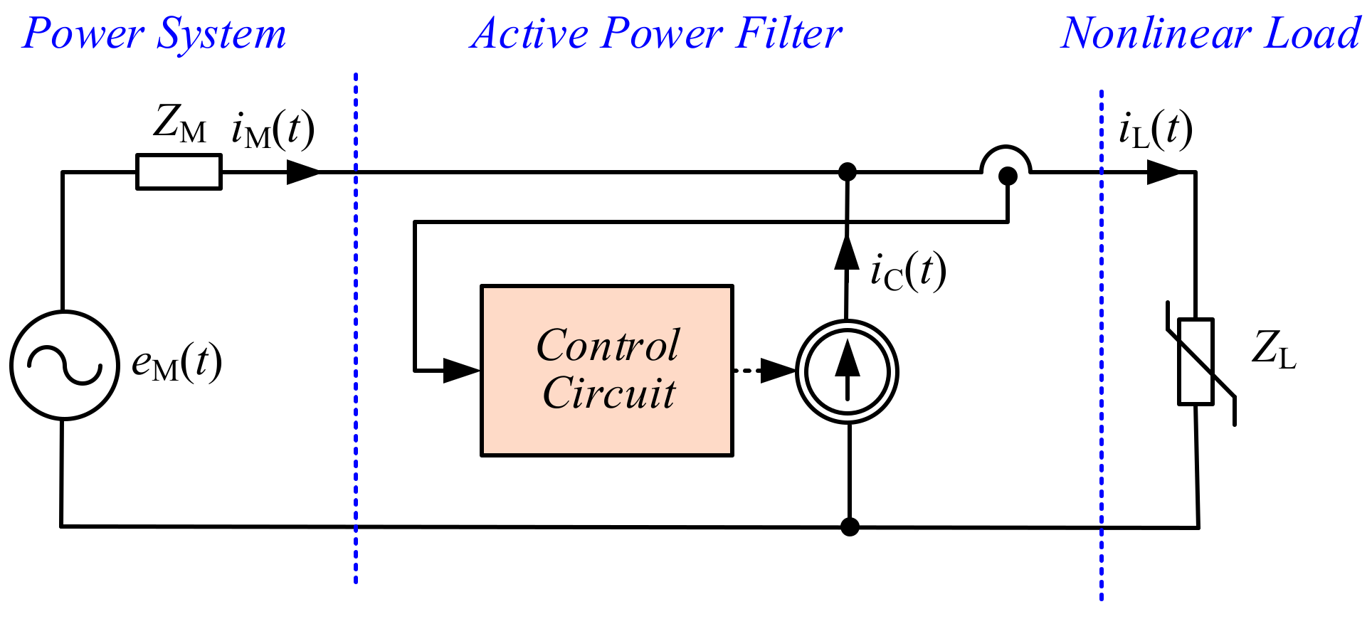
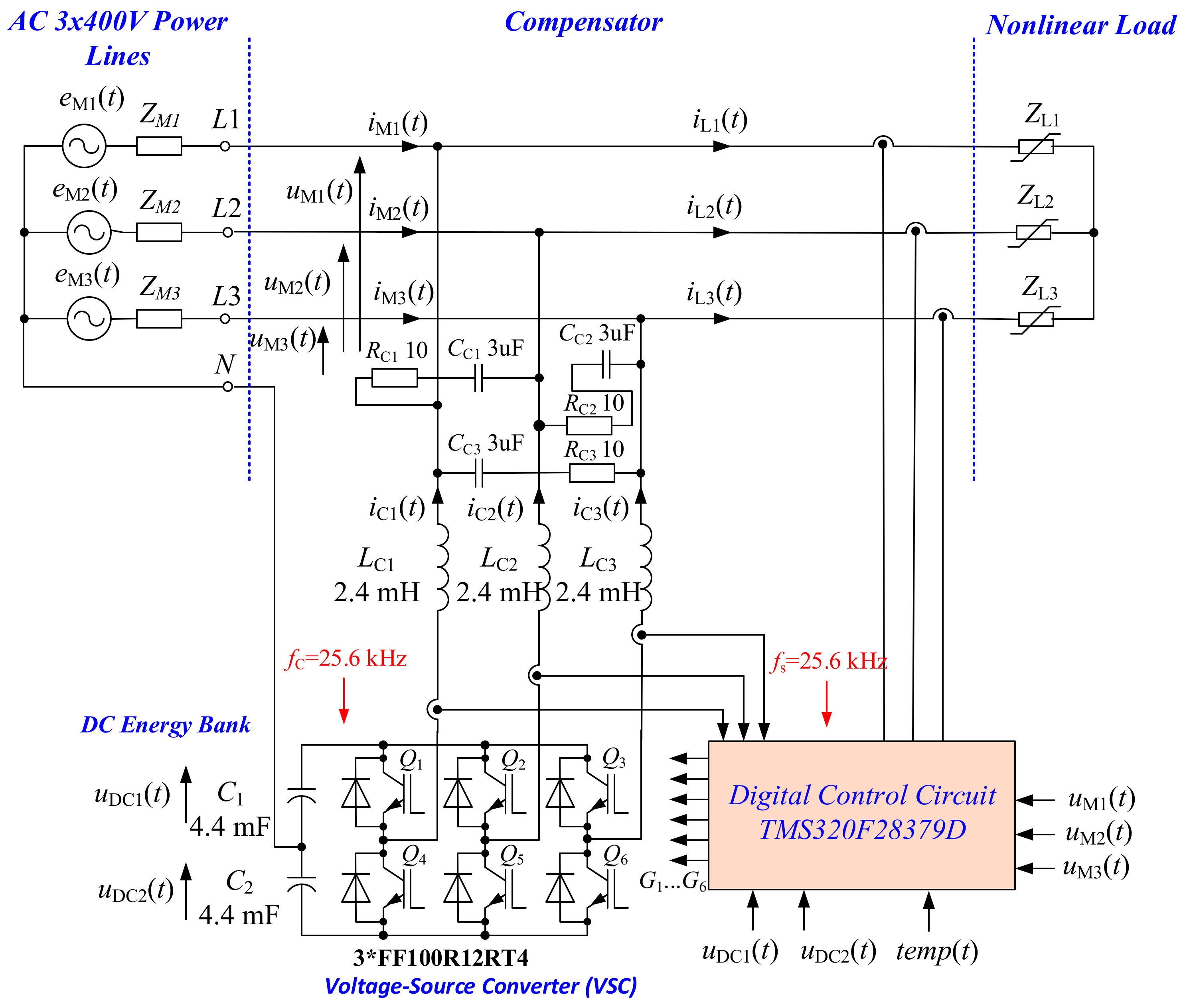
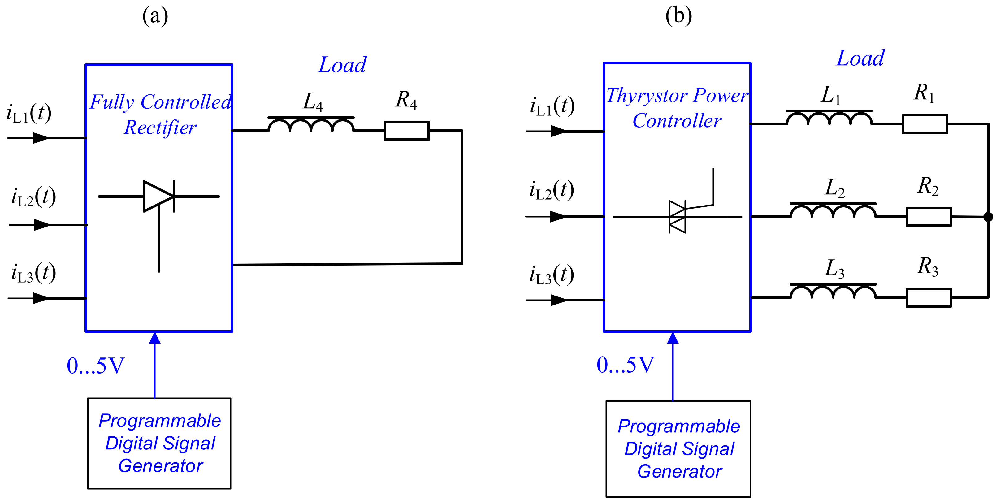
2. Circuit and Operation Description

The APF can be connected in series or in parallel with the power line. The second type, shunt APF (sometimes called: parallel APF or current-fed APF) permits compensation of the harmonics, reactive power, and asymmetries of the line currents caused by nonlinear loads.

A simplified diagram of a compensation circuit with shunt APF without feedback is shown in Figure 1. The APF has unity gain and was chosen because of its assured stability in use.

The shunt APF injects compensation current i_C(t) to cancel out the power line current harmonics content and reactive power. The resulting line current i_M(t) is the sum of the load current i_L(t) and the compensation current i_C(t):

$$i_M\left(t\right)=i_L\left(t\right)-i_C\left(t\right)$$

(1)

In the case of full compensation of reactive power and harmonics, the compensation current can be determined by

$$i_C\left(t\right)=i_L\left(t\right)-I_{H1}\sin \left(2\pi f_{M}t\right)$$

(2)

where: I_H1—amplitude of first harmonic of load current, f_M—power line frequency.

Substituting the Equation (2) into the Equation (1), the following can be obtained:

$$i_M\left(t\right)=i_L\left(t\right)-i_L\left(t\right)+I_{H1}\sin \left(2\pi f_{M}t\right)=I_{H1}\sin \left(2\pi f_{M}t\right)$$

(3)

As a result, full compensation of reactive power and harmonics is achieved.

The purpose of this paper is to present the project, its implementation, and the results of the APF research. In the design process, the following assumptions were made:

• Compensation of line current harmonics;
• Compensation of reactive power;
• Application of the sliding DFT in control algorithm;
• Implementation of the control system using the TMS320F28379D DSP microcontroller;
• Maximum amplitude of compensation current i_C(t) is limited to 50 A;

A simplified diagram of the proposed three-phase APF compensation system is shown in Figure 2. In the APF power circuit, in order to obtain better dynamic parameters, a high transistor switching frequency f_c = 25.6 kHz was adopted, therefore fast IGBT should be used. In the APF IGBT FF100R12RT4, transistors from Infineon are used. The APF control circuit is based on the TMS320F28379D DSP microcontroller [49]. To simplify the design process, a module using the C2000 Delfino MCU F28379D LaunchPad is used [50]. In the design process, the assumption was made to maximize the use of the resources of this microcontroller with the smallest possible number of additional integrated circuits.

The APF inverter circuit is powered from a DC bank. The DC bank contains two sets of capacitors, C₁ and C₂ (Figure 2). It was assumed that the rated operating voltages of these capacitors is equal to 400V.

The shunt APF output circuit acts as a digitally controllable current source. The output circuit is constructed using a three-phase transistor inverter as depicted in Figure 2. The output circuit acts as a voltage source inverter, and therefore it must be converted into a digitally controlled current source. In this solution the digital current controller and the output inductors L_C1, L_C2, and L_C3 should be used. Additional filters R_C1C_C1, R_C2C_C2 and R_C3C_C3 are used to improve the EMC properties of the device. The main parameters of the designed APF are presented in

Table 1. Main parameters of the APF system.

Symbol	Value
C1, C2	4.4 mF/450 V
LC1, LC2, LC3	2.4 mH/50 A
CC1, CC2, CC3	3 µF/1200 V
RC1, RC2, RC3	10 Ω/10 W
fc	25,600 Hz
fs	25,600 Hz
iC1max, iC2max, iC3max,	50 A
uDC1, uDC2	400 V
Q1…Q6	IGBT FF100R12RT4
MCU	TMS320F28379D, 100 MHz

.

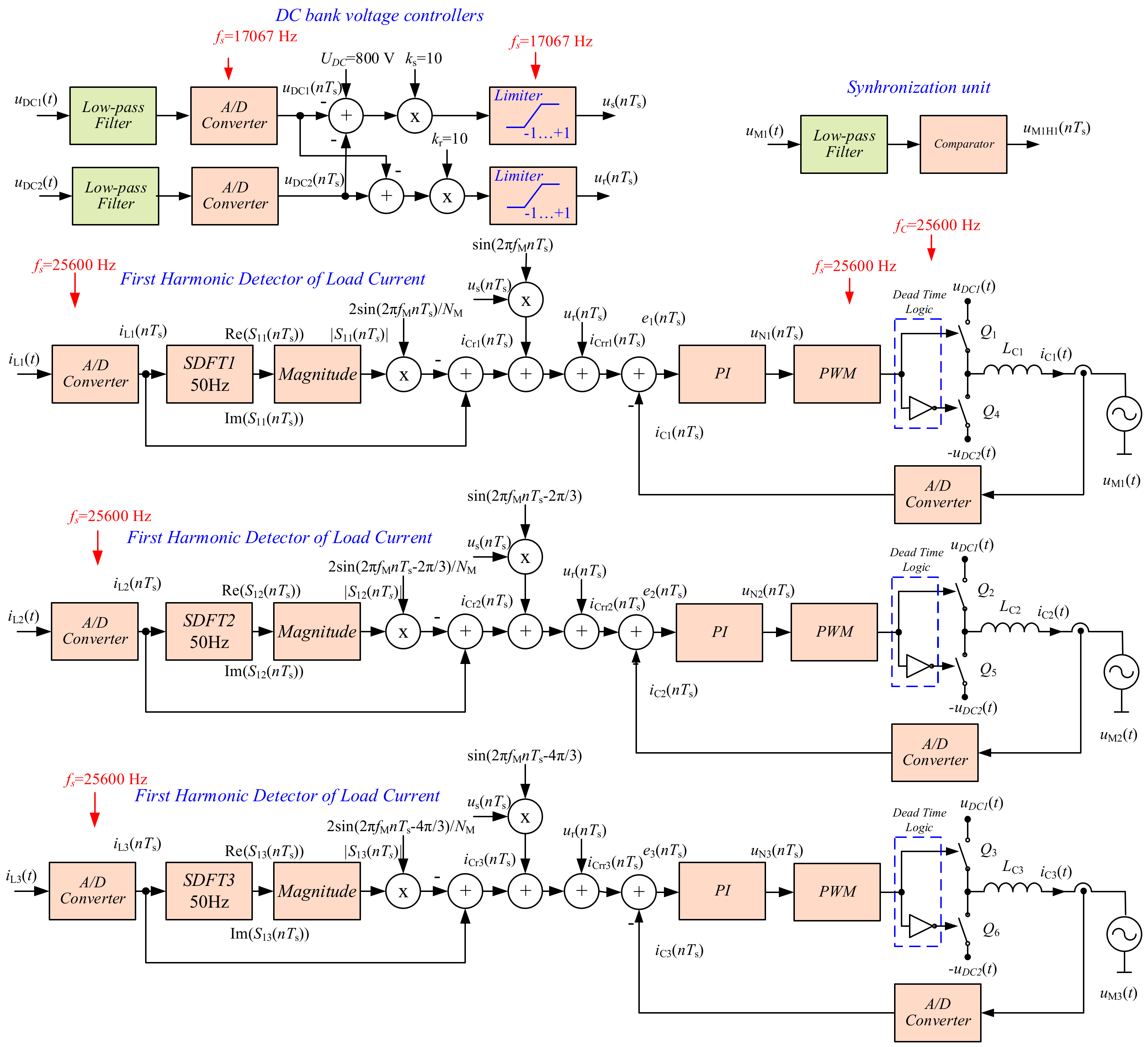
3. Control Circuit of APF

The simplified block diagram of a control circuit is depicted in Figure 3. It has twelve analog inputs: signals from currents i_C1(t), i_C2(t), i_C3(t), i_L1(t), i_L2(t), and i_L3(t), signals from voltages u_DC1(t), u_DC2(t), u_M1(t), u_M2(t), and u_M3(t), and signal from radiator temperature sensor temp(t). The current signals are generated by galvanically isolated high precision linear current sensors, the IC ACS770LCB-050B from Allegro [51]. The device consists of a precision, low-offset linear Hall circuit with a copper conduction path located near the die. The sensors are supplied by +5 V source. Signals from current sensors are connected to microcontroller input by resistor divider to reduce voltage range to 0…3.3 V.

For galvanic isolation of voltage input signals the AMC1311 integrated circuits [52] are used. The AMC1311 is a precision, isolated amplifier with an output separated from the input circuitry by a capacitive isolation barrier. Its advantage is that it is highly resistant to magnetic interference. It is also important that this barrier is certified to provide reinforced galvanic isolation of up to 5 kV_RMS AC-cording to standards DIN EN IEC 60747-17 (VDE 0884-17) and UL1577 and supports a working isolation voltage of up to 1500 V_RMS. It has common mode transient immunity (CMTI) better than 100 kV/µs. So, according to its high EMC immunity, it is highly recommended for power electronics applications.

The control circuit generates signals that control the gates of the inverter transistors. It uses drivers with galvanic isolation type 2ED020I12FA from Infineon. For driver supply, DC/DC MGJD121509SC converters are used, which convert the 12 V voltage into galvanically isolated voltages of +15 V and −8 V.

A view of the APF control circuit, during the development process (during desktop testing), is shown in Figure 4.

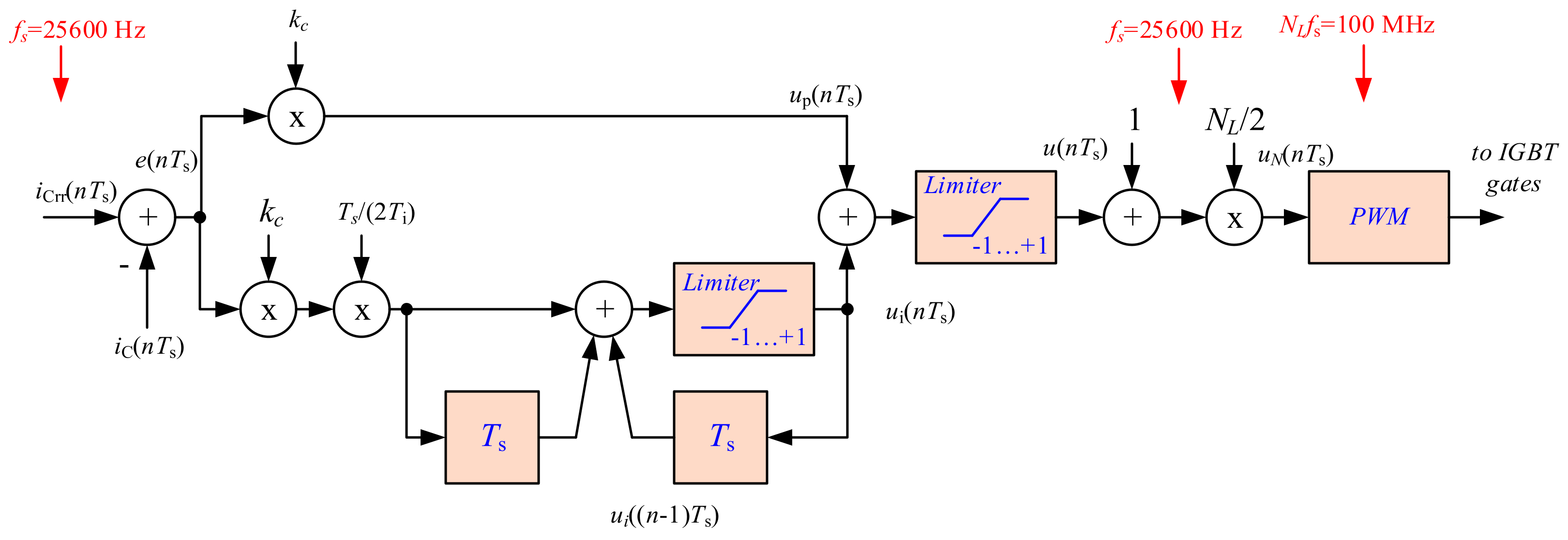
3.1. Control Algorithm

The APF system should ensure compensation of reactive power and harmonics. A simplified block diagram of the control algorithm that meets these requirements is shown in Figure 3. The control circuit consists of a few control loops.

Two digital proportional controllers are used to stabilize and symmetrize DC bank voltages and three digital output current PI controllers (Figure 3).

An algorithm based on sliding DFT is used to determine the first harmonic of the load current [26,37,38].

Due to the high stability of the power line frequency, the deviation is typically less than +/− 50 mHz [53], and the use of the phase lock loop (PLL) circuit has been abandoned. Thanks to this, low frequency oscillations associated with the reaction of the PLL system to disturbances in the supply network are avoided. Instead, a low-pass filter was applied to the u_M1(t) voltage signal and zero-crossing detection to achieve synchronization of the control algorithm. The phase shift of the synchronization signal, which is introduced by the low-pass filter, is compensated digitally.

3.2. Digital Current Controller

The block diagram of the digital current PI controller is depicted in Figure 5. Below is the transfer function of the PI controller

$$H\left(z\right)=k_C+k_C\frac{T_s}{2T_i}\frac{1+z^{-1}}{1-z^{-1}}$$

(4)

where: k_C—controller gain, T_i—integrator time constant, T_s—sampling period.

Using the controller transfer function (4), it is possible to obtain the difference equation of the control signal:

$$u\left(n\right)=k_{C}e\left(n\right)+\stackrel{sum\left(n\right)}{\overbrace{k_C\frac{T_s}{2T_i}\left(e\left(n\right)+e\left(n-1\right)\right)+sum\left(n-1\right)}}$$

(5)

where: e(n) = i_Crr(n) − i_C(n) —error.

In the next step, the input signal of the PWM modulator is calculated:

$$u_N\left(n\right)=1+0.5N_{L}u\left(n\right)$$

(6)

where: N_L—number of PWM modulator states.

In Equations (5) and (6), the influence of the amplitude limiter has been neglected.

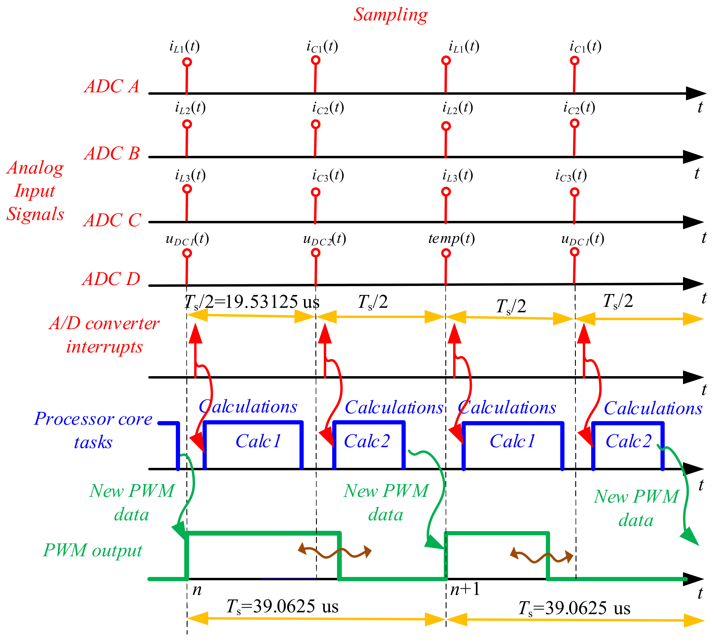
3.3. Analog Signal Sampling

As described above, the conversion of 12 analog signals is necessary to control the power circuit. Only nine signals were selected for A/D conversion, and the conversion of three supply line voltages are omitted. The signals representing currents are fast-varying, and the signals representing, e.g., DC bank voltages and temperatures are slow-varying. Hence, the best solution would be to use A/D converters with simultaneous sampling of current signals. The control circuit requires a minimum of six A/D converters with simultaneous sampling. Unfortunately, the TMS320F28379D has only four 12-bit A/D converters with simultaneous sampling [49]. Due to this, a hybrid solution was implemented in the control system that combines simultaneous and sequential sampling techniques. The sampling frequency of current signals was assumed to be equal to the switching frequency of the inverter transistors, f_s = 25.6 kHz. On the other hand, the frequency of the A/D converter operation was assumed to be twice as high. The process of sampling all signals consists in three cycles; these are described in

Table 2. Sampling cycles.

Sampling Cycle	ADC Channel A	ADC Channel B	ADC Channel C	ADC Channel D
1	iL1(t)	iL2(t)	iL3(t)	uDC1(t)
2	iC1(t)	iC2(t)	iC3(t)	uDC2(t)
3	iL1(t)	iL2(t)	iL3(t)	temp(t)

. In summary, current signals are sampled at the f_s frequency, while voltage and temperature signals are sampled at the frequency of 2/3f_s = 17,066 Hz.

It is very important that the sampling process is triggered by an internal counter in the microcontroller with a constant and stable sampling rate of 2 f_s = 51.2 kHz. This solution minimizes jitter, which deteriorates the signal-to-noise ratio [26].

The entire control algorithm is executed during the interrupt generated by the A/D converter. The four A/D converters can operate in simultaneous sampling mode with a sampling rate of 2f_s = 51.2 kHz. The timing diagram of data flow in the APF control circuit is depicted in Figure 6. The sampling period is equal to T_s/2 = 19.53125 µs, thus, the execution time of the interrupt program must be shorter. This time is too short to implement the whole control algorithm, so it has been divided into two parts, Calc 1 and Calc 2. The tasks for Calc 1 and Calc 2 have been divided so as to obtain almost equal use of the interrupt duration and is about 15 µs. This solution allowed for good use of the microcontroller’s capabilities.

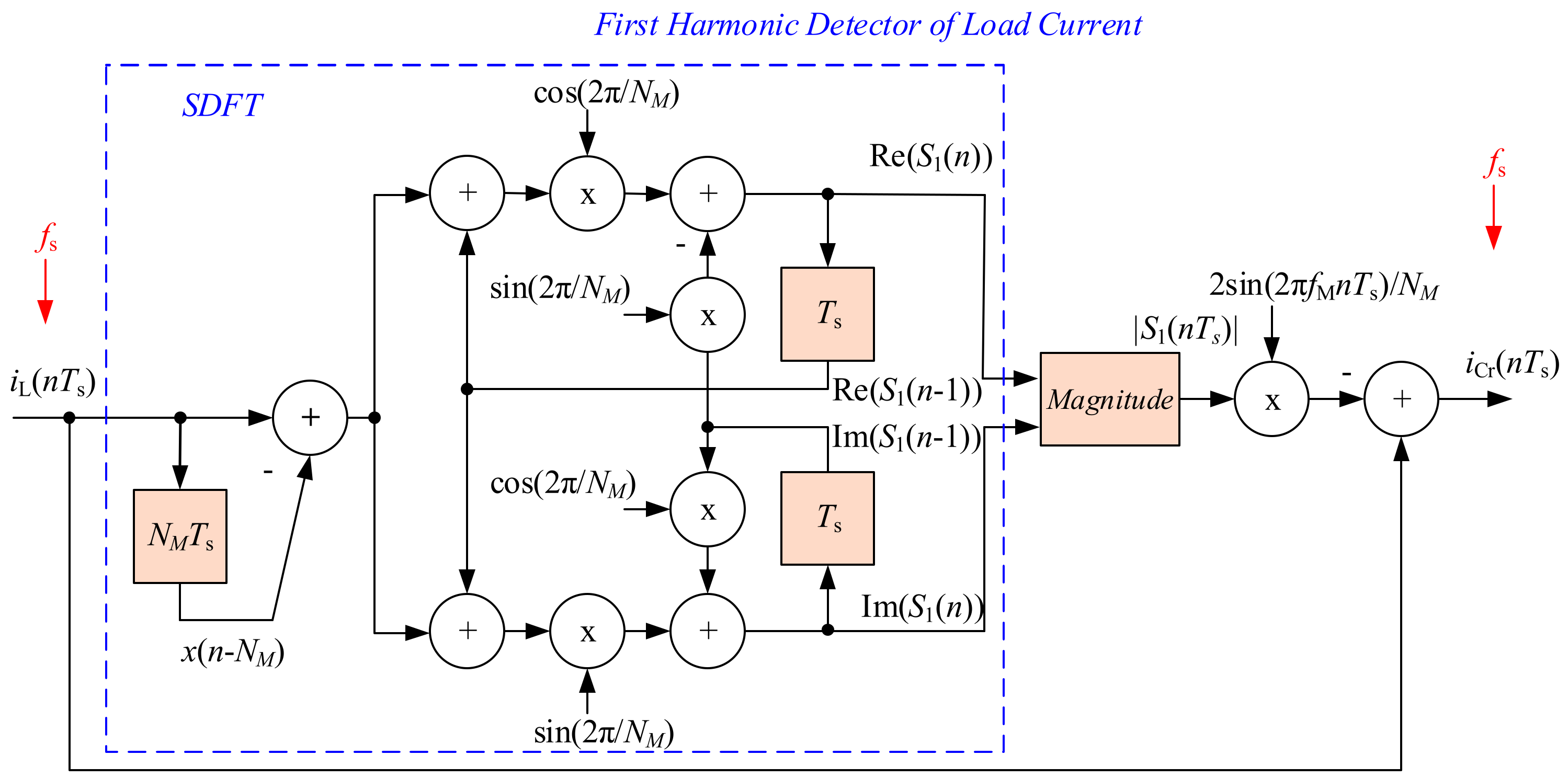
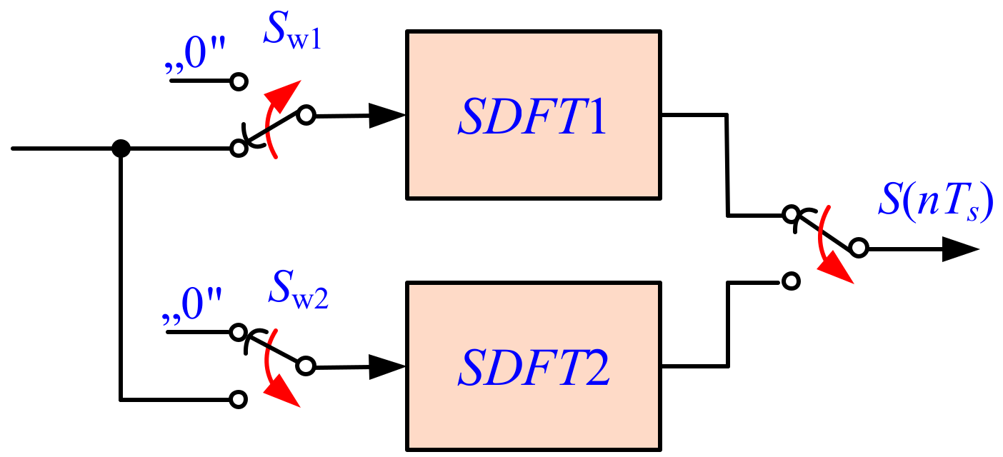
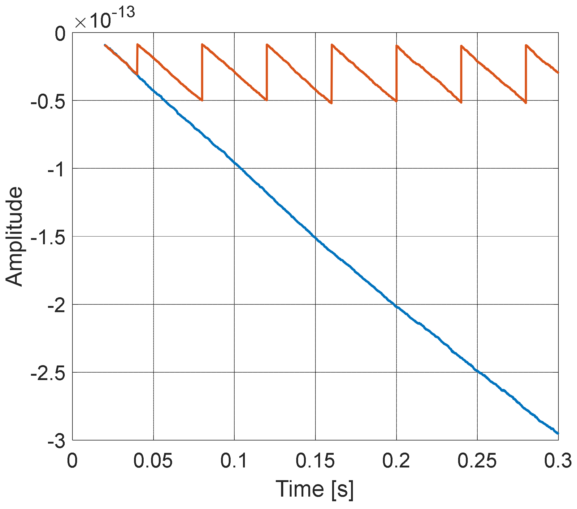
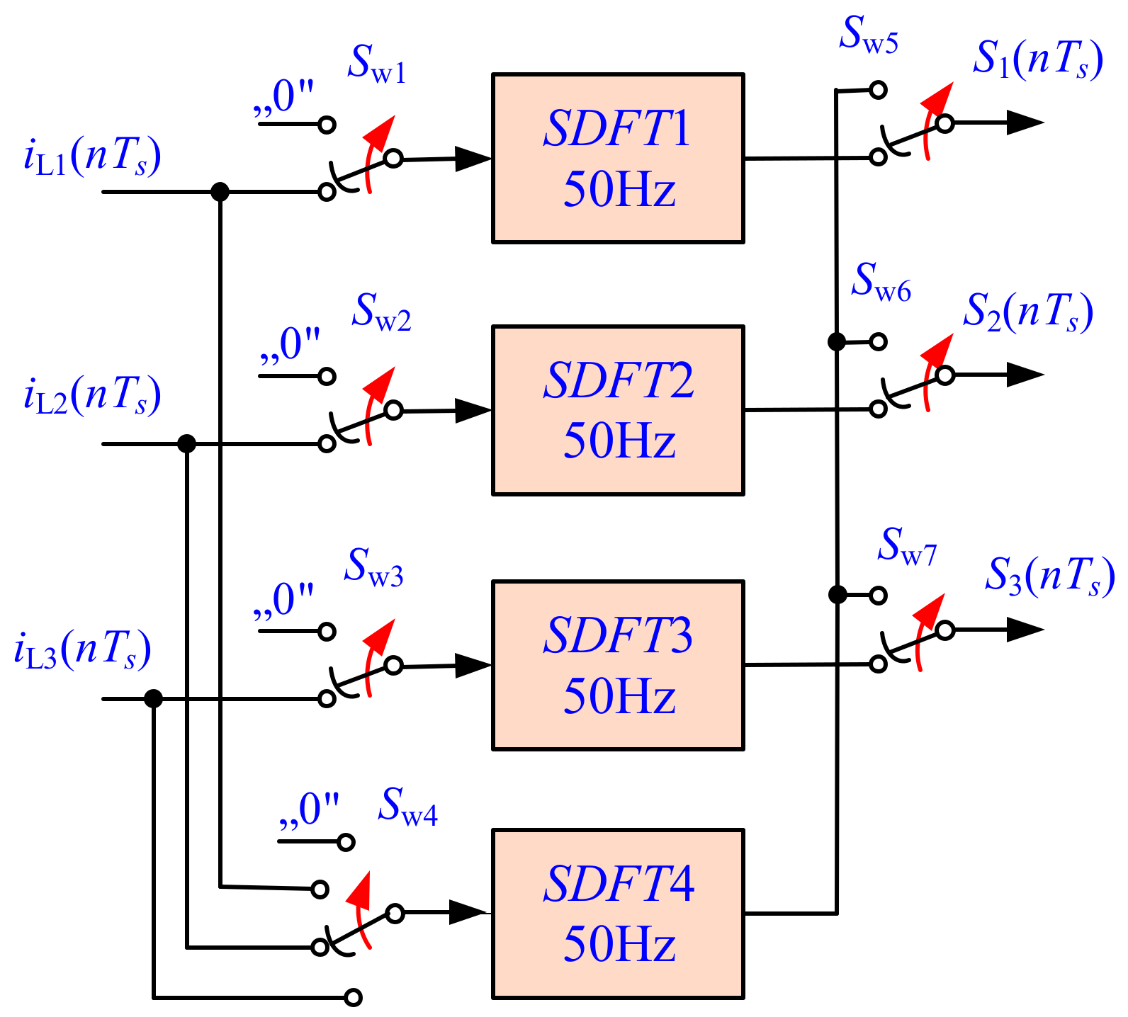
3.4. Sliding DFT Algorithm

The sliding DFT (SDFT) algorithm is featured in publications [26,27,28,29,30,31,32,33,34,35,36,37,38,39,40,41,42,43,44,45,46,47,48,49,50,51,52,53]. The SDFT algorithm is useful for using in APF control circuits [26,37,38]. The principle of the algorithm is considered in publications [26,27,28,29]. For detecting the first harmonic of load current, only one signal-bin SDFT filter structure is used. The first harmonic spectral component signal of load current is calculated

$$S_1\left(n\right)=e^{\mathrm{j}2\mathsf{\pi }k/N_M}\left(S_1\left(n-1\right)-i_L\left(n-N_M\right)+i_L\left(n\right)\right)$$

(7)

where: S₁(n)—discrete signal representing first harmonic complex spectral component of load current, N_M—number samples per line period.

The discrete signal representing the load current first harmonic with zero phase angle between line voltage u_M(t) and line current i_H1(n):

$$i_{H1}\left(n\right)=2/N_M\left|S_1\left(n\right)\right|\sin \left(2\mathsf{\pi }50n{T}_s\right)$$

(8)

Finally, compensation current signal is the result of a difference between the load current signal and the first harmonic sinusoidal signal of load current:

$$i_{Cr}\left(n\right)=i_L\left(n\right)-2/N_M\left|S_1\left(n\right)\right|\sin \left(2\mathsf{\pi }50n{T}_s\right)$$

(9)

The block diagram of the circuit for calculating compensation current is depicted in Figure 7. The algorithm based on SDFT gave very good results during simulation tests and during preliminary laboratory tests. However, during long-term laboratory tests, it turned out that this approach produced a serious numerical error that causes a continuous decrease in the amplitude of the fundamental component. A significant error of the SDFT algorithm occurred after several dozen minutes of APF operation during laboratory tests. This was confirmed during additional simulation studies in Matlab.

It is possible to find many publications devoted to the stabilization method of the SDFT algorithm. For example, the works of Lyons, Duda, and many others [33,34,35,36,37,38]. However, these methods fail for the single precision floating point used in the microcontroller. The authors used their original solution to the problem. The SDFT algorithm has a response settling time equal to N_M∙T_s, i.e., one power line period. This solution consists of two SDFT circuits switched alternately. A block diagram of this switching SDFT (SSDFT) is shown in Figure 8. The working principle of SSDFT is described in

Table 3. Working principle of SSDFT.

State Number	Line Period	SDFT1	SDFT2
1	1	IL -> S	0
2	1	IL -> S	IL
3	1	0	IL -> S
4	1	IL	IL -> S

.

The complete SSDFT concept has been thoroughly tested using simulation testing in Matlab and Psim. The simulation work confirmed that SSDFT works as intended, without a continuous increase in numerical errors. Figure 9 shows a waveform of magnitude error |S₁(nT_s)| (see Figure 7) for unity input signal. Waveforms of the classical approach are shown in blue, whereas the SSDFT approach is marked in red. As can be seen in Figure 9, the error continues to increase throughout the operation of the classical SDFT circuit, whereas the error is constrained for the SSDFT. The difference is that the SSDFT circuit is periodically reset, thanks to which the error does not grow.

In subsequent tests, SSDFT implementation was tested experimentally using the TMS320F28379D microcontroller. To date, extensive experimental tests have confirmed the stability of this implementation.

The SSDFT concept was utilized in the design of three-phase first harmonic detectors. A block diagram of these detectors using a stable SSDFT is depicted in Figure 10. The principle of operation is shown in

Table 4. The principle of three-phase SSDFT operation.

State Number	The Number of Line Period	SDFT1	SDFT2	SDFT3	SDFT4
1	8	IL1 -> S1	IL2 -> S2	IL3 -> S3	0
2	1	IL1 -> S1	IL2 -> S2	IL3 -> S3	IL1
3	8	0	IL2 -> S2	IL3 -> S3	IL1 -> S1
4	1	IL1	IL2 -> S2	IL3 -> S3	IL1 -> S1
5	8	IL1 -> S1	IL2 -> S2	IL3 -> S3	0
6	1	IL1 -> S1	IL2 -> S2	IL3 -> S3	IL2
7	8	IL1 -> S1	0	IL3 -> S3	IL2 -> S2
8	1	IL1 -> S1	IL2	IL3 -> S3	IL2 -> S2
9	8	IL1 -> S1	IL2 -> S2	IL3 -> S3	0
10	1	IL1 -> S1	IL2 -> S2	IL3 -> S3	IL3
11	8	IL1 -> S1	IL2 -> S2	0	IL3 -> S3
12	1	IL1 -> S1	IL2 -> S2	IL3	IL3 -> S3

. Compared to the classical three-phase SDFT algorithm, the three-phase SSDFT requires only about 25% more arithmetic operations.

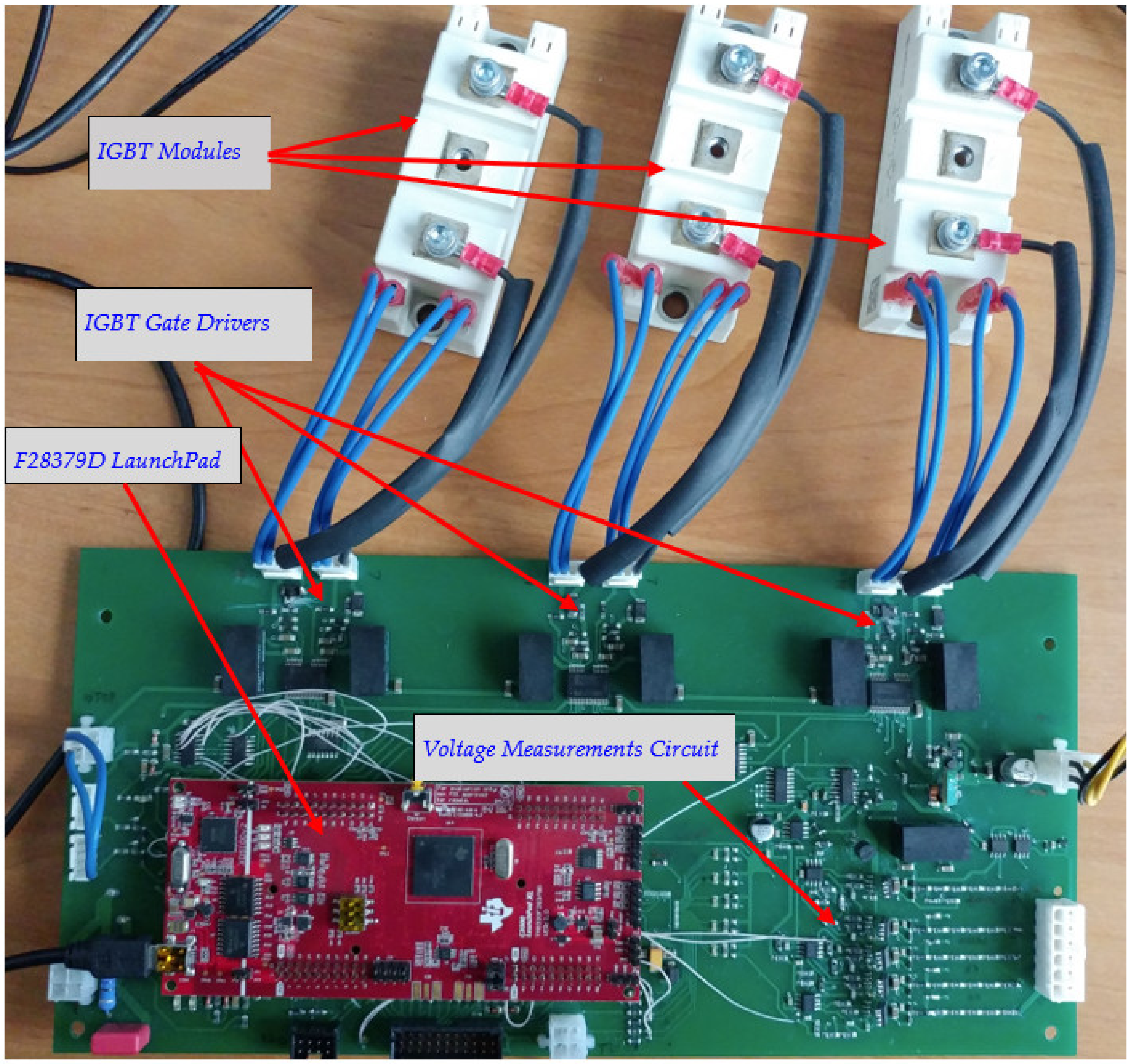
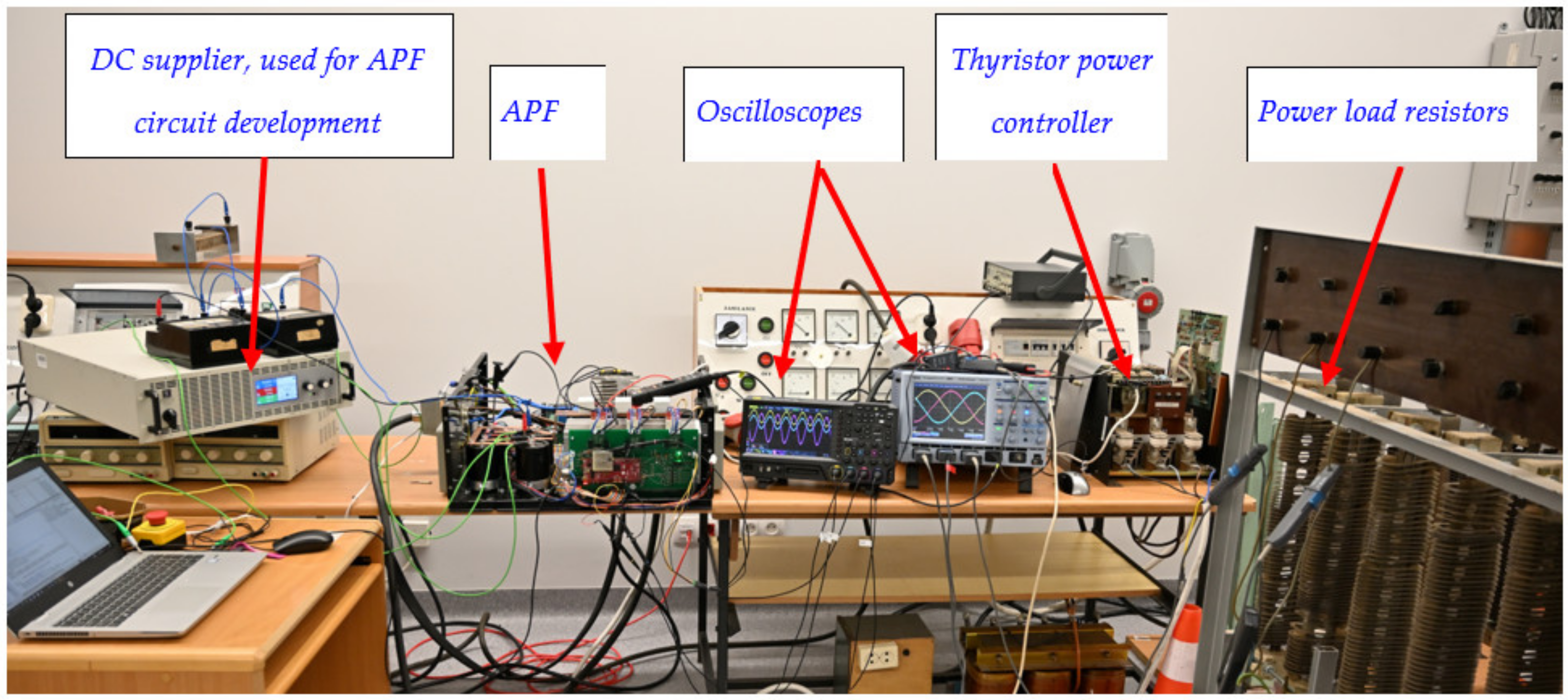
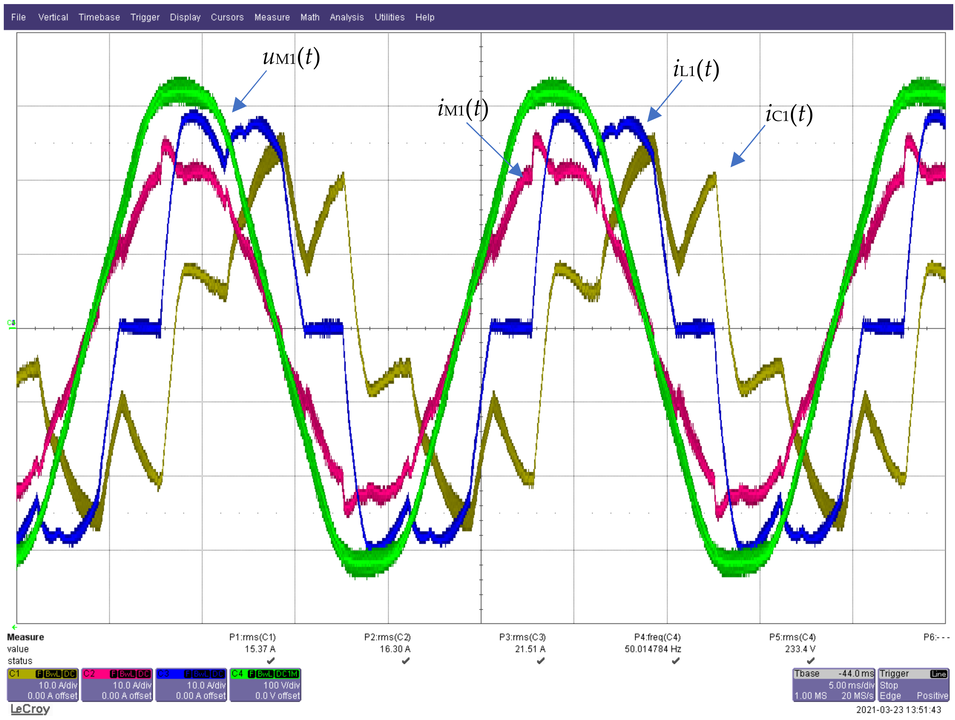
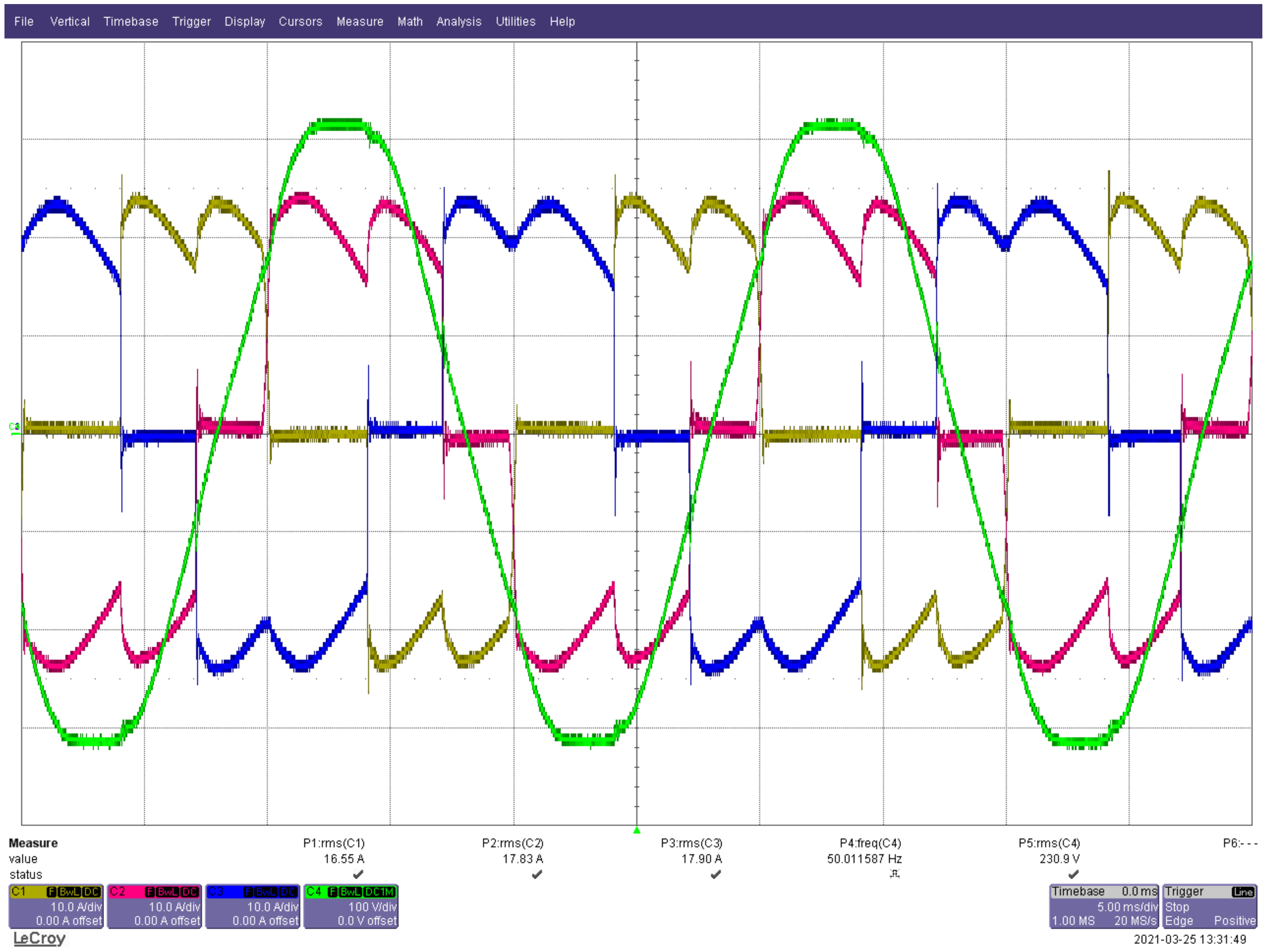
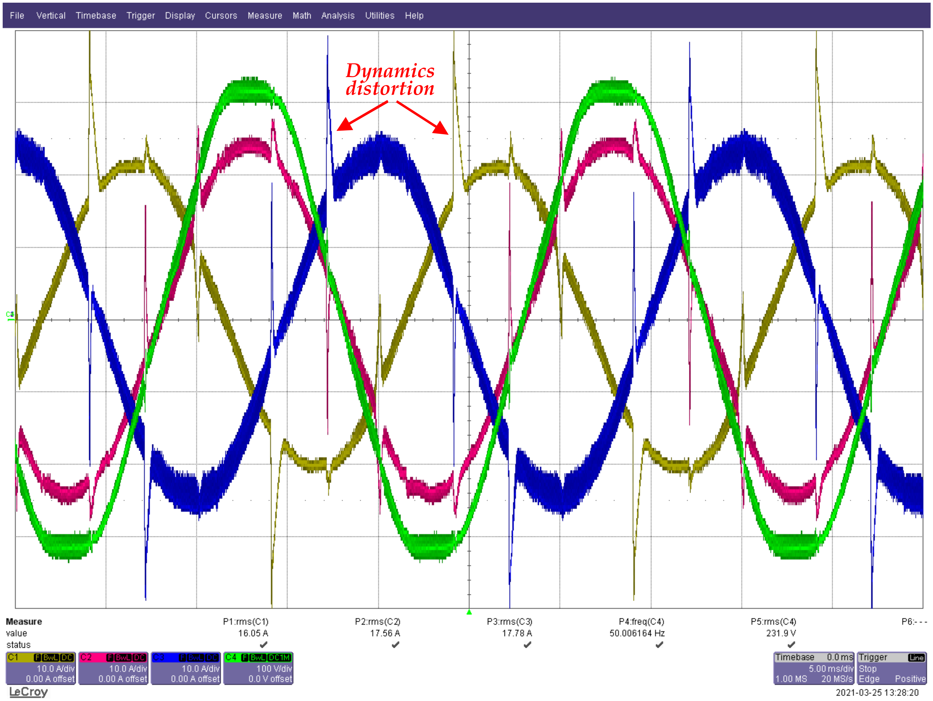
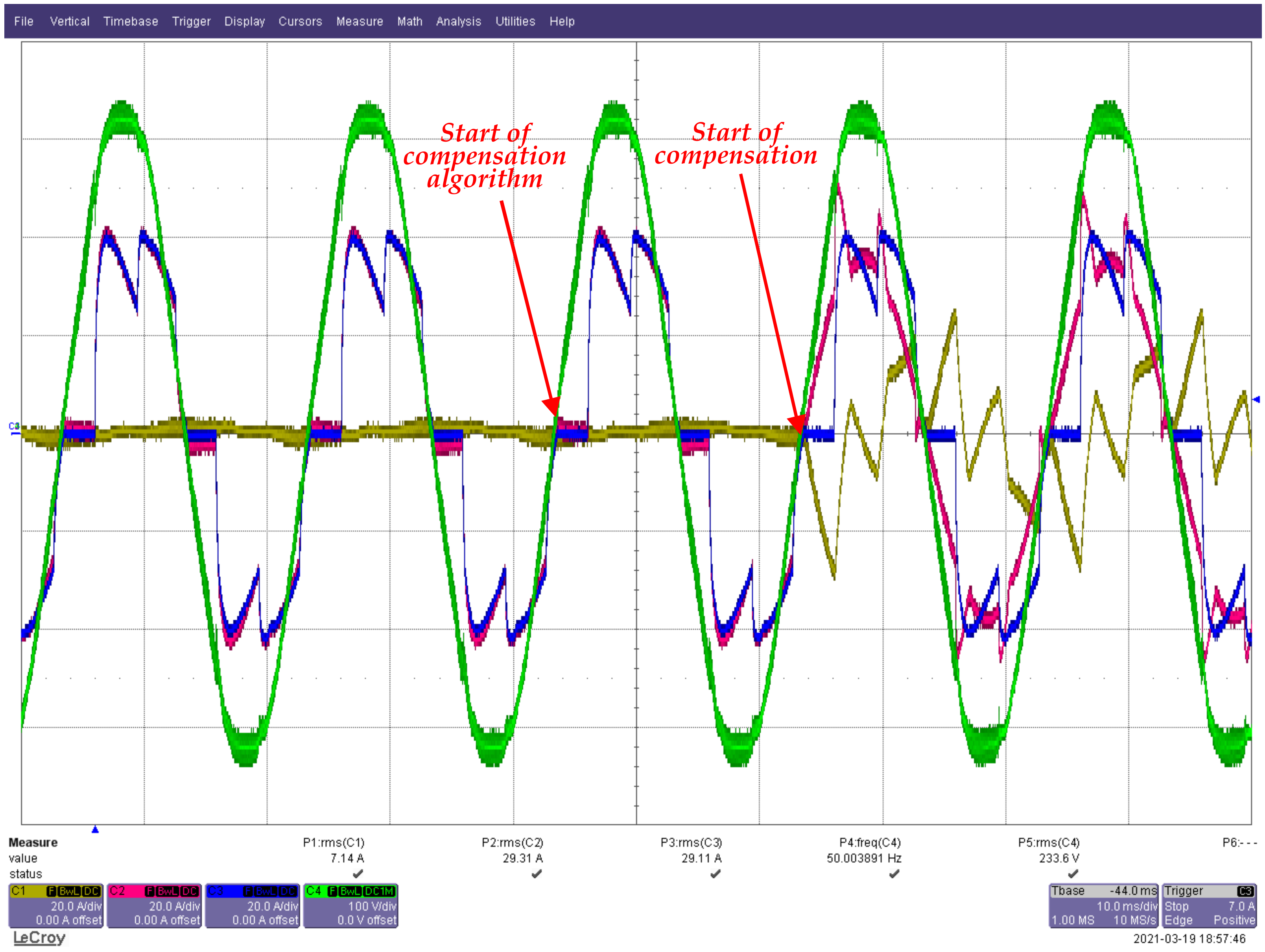
4. Laboratory Test of the APF

The described APF was built and tested experimentally. The view of the laboratory setup is shown in Figure 11. The operation of the APF has been intensively tested in the laboratory for two non-linear loads. The diagram of the loads used in laboratory test are depicted in Figure 12. The three-phase power controller with R and RL load shown in Figure 12a, and the three-phase thyristor-controlled rectifier with R and RL load is shown in Figure 12b. In both cases, positive results of the APF work were obtained.

The APF control current dynamics is mainly dependent on the power inverter output circuit time constant, resulting from APF output inductance and resultant impedance of load and mains. Exemplary experimental waveforms of APF in steady state for nonlinear load with a three-phase thyristor power controller with RL loads are shown in Figure 13—line current i_M1(t), compensation current i_C1(t), load current i_L1(t), and line voltage u_M1(t). As can be seen in Figure 13, line voltage and current have zero-degree phase shift, signifying that the reactive power was fully compensated. When the value of load current changes rapidly, as in current i_L1(t) in Figure 13, the APF transient response is too slow [26,54], and the line current i_M1(t) suffers from dynamic distortion. This distortion causes an increase in harmonic content in the line current. The presence of these distortions increases the value of the total harmonics distortion ratio (THD) of the line current by about 10% [26,54]. The solution to this problem using a predictive control algorithm is presented separately by the author in [54]; this approach can also be combined with SSDFT.

Shown in Figure 14 and Figure 15 are experimental three-phase waveforms of the APF in steady state for load with fully controlled rectifier. Figure 15 also shows the dynamic distortion of the line current resulting from the delay introduced by the inductors. It should be noted that, in the tested load, the rate of current changes is much higher than in typical industrial loads.

Figure 16 illustrates the transient behavior of the APF. As you can see, from the moment the compensation algorithm is switched on to obtaining a full compensation, one period of the power supply network is needed.

The operation of the APF for time-varying load current values is shown in a short video posted on the author’s website [55]. The following waveforms are shown there: load current i_L1(t) (magenta), compensation current i_C1(t) (green), and line current i_M1(t) (yellow). As you can see there, the APF performs well for changing load current.

5. Discussion and Conclusions

The presented method of the implementation of a limited number of A/D converters with simultaneous sampling was practically tested using both simulation and experimental work. This strategy allowed for a full use of the microcontroller’s capabilities, without using any external A/D converters. Using the Delfino MCU F28379D LaunchPad module significantly simplified and accelerated the process of printed board design.

Use of the SSDFT algorithm allowed for agile and reliable SDFT implementation employing a microcontroller with only a single precision floating point arithmetic. The effectiveness of the whole APF was rigorously tested during extensive laboratory testing.

The design and development process of APF is one of the most difficult issues due to the fact that the power supply of the system is from the DC bank. In order for the DC bank to work, the current controllers and DC voltage controllers must work properly. In a DC system, the bank very easily obtains a voltage higher than the permissible voltage of capacitors, which can lead to their destruction, especially if the operating voltage of the capacitors is close to their maximum voltage. Overvoltage can be achieved very easily when creating and debugging a program for a microcontroller. Therefore, it is worth introducing hardware overvoltage protection.

Summing up, the most important contributions of the paper are:

• Development of a method for stabilizing the SDFT algorithm for implementation using single precision floating point;
• The three-phase SSDFT requires only about 25% more arithmetic operations than classic SDFT;
• Development of a method for sampling signals using a limited number of sample and hold systems;
• The sample and hold circuits are triggered by a hardware counter, which minimizes the jitter phenomenon.
• Design and implementation of a complex and difficult device, such as APF.

Currently, the APF is used intensively to research new control algorithms.

Future work in the area could include output LCL filter implementation. The LCL filter would permit reduction in the level of current ripples and would improve dynamic properties of the APF.

References

1. Ciok, Z.; Królikowski, L.; Nowakowski, R.; Szymczak, P. Michał Doliwo-Dobrowolski-Współtwórca Cywilizacji Technicznej XX Wieku; Wiadomości Elektrotechniczne: Warsaw, Poland, 2009; R. 77, nr 1; pp. 38–49. (In Polish) [Google Scholar]
2. Available online: https://bezel.com.pl/2016/11/24/michal-doliwo-dobrowolski/ (accessed on 5 January 2023).
3. Available online: https://en.wikipedia.org/wiki/Mikhail_Dolivo-Dobrovolsky (accessed on 5 January 2023).
4. Klug, W. Die Elektrische Kraftűbertragungsanlage Eichdorf—Grünberg in Schl.; Elektrotechnische Zeitsdrift (ETZ): Berlin, Germany, 1896; H. 45; pp. 686–689. [Google Scholar]
5. Bird, B.; Marsh, J.; McLellan, P. Harmonic reduction in multiple converters by triple-frequency current injection. IEEE Proc. 1969, 116, 1730–1734. [Google Scholar]
6. Gyugi, L.; Strycula, E. Active ac Power Filters. In Proceedings of the IEEE IAS Annual Meeting, Chicago, IL, USA, 11–14 October 1976; pp. 529–535. [Google Scholar]
7. Mohan, N.; Peterson, H.; Long, W.; Dreifuerst, G.; Vithaythil, J. Active Filters for AC Harmonic Suppression. In Proceedings of the IEEE/PES Winter Meeting, New York, NY, USA, 30 January–4 February 1977. [Google Scholar]
8. Uceda, J.; Aldana, F.; Martinez, P. Active filters for static power converters. IEEE Proc. B 1983, 130, 347–354. [Google Scholar]
9. Kawahira, H.; Nakamura, T.; Nakazawa, S.; Nomura, M. Active Power Filter. In Proceedings of the International Power Electronics Conference, Tokyo, Japan, 27–31 March 1983; pp. 981–992. [Google Scholar]
10. Akagi, H.; Kanazawa, Y.; Nabae, A. Generalized Theory of the Instantaneous Reactive Power in Three-Phase Circuits. In Proceedings of the International Power Electronics Conference, Tokyo, Japan, 27–31 March 1983; pp. 1375–1386. [Google Scholar]
11. Akagi, H.; Tsukamoto, Y.; Nabae, A. Analysis and design of an active power filter using quad-series voltage-source PWM converters. IEEE Trans. Ind. Appl. 1990, 26, 93–98. [Google Scholar] [CrossRef]
12. Peng, F.; Akagi, H.; Nabae, A. A study of active power filters using quad-series voltage-source PWM converters for harmonic compensation. IEEE Trans. Power Electron. 1990, 5, 9–15. [Google Scholar] [CrossRef]
13. Moran, S. A Line Voltage Regulator/Conditioner for Harmonic Sensitive Load Isolation. In Proceedings of the IEEE/IAS Annual Meeting, San Diego, CA, USA, 1–5 October 1989; pp. 947–951. [Google Scholar]
14. Akagi, H. Trends in active power line conditioners. IEEE Trans. Power Electron. 1994, 9, 263–268. [Google Scholar] [CrossRef]
15. Akagi, H. New Trends in Active Filters. In Proceedings of the International Conference on Power Electronics, Drives and Energy Systems for Industrial Growth, New Delhi, India, 8–11 January 1996; pp. 17–26. [Google Scholar]
16. Akagi, H. New Trends in Active Filters for Power Conditioning. IEEE Trans. Ind. Appl. 1996, 32, 1312–1322. [Google Scholar] [CrossRef]
17. Singh, B.; Al-Haddad, K.; Chandra, A. A review of active filters for power quality improvement. IEEE Trans. Ind. Electron. 1999, 46, 960–971. [Google Scholar] [CrossRef]
18. Peng, F.Z. Harmonic sources and filtering approaches. IEEE Ind. Appl. Mag. 2001, 7, 18–25. [Google Scholar] [CrossRef]
19. Akagi, H. Active harmonic filters. Proc. IEEE 2005, 93, 2128–2141. [Google Scholar] [CrossRef]
20. Akagi, H.; Watanabe, E.H.; Aredes, M. Instantaneous Power Theory and Applications to Power Conditioning; Wiley-IEEE Press: Hoboken, NJ, USA, 2007. [Google Scholar]
21. Benysek, G.; Pasko, M. (Eds.) Power Theories for Improved Power Quality; Springer: London, UK, 2012. [Google Scholar]
22. Afonso, J.L.; Tanta, M.; Pinto, J.G.O.; Monteiro, L.F.C.; Machado, L.; Sousa, T.J.C.; Monteiro, V. A Review on Power Electronics Technologies for Power Quality Improvement. Energies 2021, 14, 8585. [Google Scholar] [CrossRef]
23. Buła, D.; Grabowski, D.; Maciążek, M. A Review on Optimization of Active Power Filter Placement and Sizing Methods. Energies 2022, 15, 1175. [Google Scholar] [CrossRef]
24. Das, S.R.; Ray, P.K.; Sahoo, A.K.; Ramasubbareddy, S.; Babu, T.S.; Kumar, N.M.; Elavarasan, R.M.; Mihet-Popa, L. A Com-prehensive Survey on Different Control Strategies and Applications of Active Power Filters for Power Quality Improvement. Energies 2021, 14, 4589. [Google Scholar] [CrossRef]
25. Asiminoaei, L.; Blaabjerg, F.; Hansen, S. Detection is key—harmonic detection methods for active power filter applications. IEEE Ind. Appl. Mag. 2007, 13, 22–33. [Google Scholar] [CrossRef]
26. Sozanski, K. Digital Signal Processing in Power Electronics Control Circuits, 2nd ed.; Springer: London, UK, 2017. [Google Scholar]
27. Jacobsen, E.; Lyons, R. The sliding DFT. IEEE Signal Process. Mag. 2003, 20, 74–80. [Google Scholar]
28. Jacobsen, E.; Lyons, R. An update to the sliding DFT. IEEE Signal Process. Mag. 2004, 21, 110–111. [Google Scholar] [CrossRef]
29. Jacobsen, E. Understanding and Implementing the Sliding DFT, dsprelated.com. The Related Media Group. Available online: https://www.dsprelated.com/ (accessed on 5 January 2023).
30. Sherlock, B.G.; Monro, D.M. Moving discrete Fourier transform. IEE Proc. Radar Signal Process. 1992, 139, 279–282. [Google Scholar] [CrossRef]
31. Brown, A. Running Fourier Transforms; Electronics World: Maidstone, UK, 1998; p. 959. [Google Scholar]
32. Assous, S.; Linnett, L. High resolution time delay estimation using sliding discrete Fourier transform. Digit. Signal Process. 2012, 22, 820–827. [Google Scholar] [CrossRef]
33. Lyons, R. Understanding Digital Signal Processing, 3rd ed.; Prentice Hall: Upper Saddle River, NJ, USA, 2011; pp. 479–498. [Google Scholar]
34. Douglas, S.; Soh, J. A Numerically Stable Sliding-Window Estimator and Its Application to Adaptive Filters. In Proceedings of the 31st Asilomar Conference on Signals, Systems, and Computers, Pacific Grove, CA, USA, 31 October–2 November 1997; Volume 1, pp. 111–115. [Google Scholar]
35. Gufovskiy, D.; Chu, L. An accurate and stable sliding DFT computed by a modified CIC filter. IEEE Signal Process. Mag. 2017, 34, 89–93. [Google Scholar] [CrossRef]
36. Lyons, R. Streamlining Digital Signal Processing: A Tricks of the Trade Guide-Book; Wiley: Hoboken, NJ, USA, 2012. [Google Scholar]
37. Sozanski, K.; Jarnut, M. Three-Phase Active Power Filter Using the Sliding DFT Control Algorithm. In Proceedings of the 11th European Conference on Power Electronics and Applications, Dresden, Germany, 11–14 September 2005. [Google Scholar]
38. Sozanski, K. Harmonic Compensation Using the Sliding DFT Algorithm. In Proceedings of the IEEE 35th Annual Power Electronics Specialists Conference —PESC ’04, Aachen, Germany, 20–25 June 2004. [Google Scholar]
39. Lyons, R.; Howard, C. Improvements to the Sliding Discrete Fourier Transform Algorithm. IEEE Signal Process. Mag. 2021, 38, 119–127. [Google Scholar] [CrossRef]
40. Duda, K. Accurate, guaranteed stable, sliding discrete Fourier transform. IEEE Signal Process. Mag. 2010, 27, 124–127. [Google Scholar]
41. Park, C.S. Fast, accurate, and guaranteed stable sliding discrete Fourier transform. IEEE Signal Process. Mag. 2015, 32, 145–156. [Google Scholar] [CrossRef]
42. Li, K.; Nai, W. Rapid Extraction of the Fundamental Components for Non-Ideal Three-Phase Grid Based on an Improved Sliding Discrete Fourier Transform. Electronics 2022, 11, 1915. [Google Scholar] [CrossRef]
43. Tan, G.; Fu, Q.; Xia, T.; Zhang, X. Development of Frequency Fixed Sliding Discrete Fourier Transform Filter Based Single-Phase Phase-Locked Loop. IEEE Access 2021, 9, 110573–110581. [Google Scholar] [CrossRef]
44. Orallo, C.M.; Carugati, I. Single Bin Sliding Discrete Fourier Transform. In Fourier Transforms—High-Tech Application and Current Trends; Nikolic, G.S., Cakic, M.D., Cvetkovic, D.J., Eds.; IntechOpen: London, UK, 2017. [Google Scholar] [CrossRef] [Green Version]
45. Kulshreshtha, T.; Dhar, A.S. Improved VLSI architecture for triangular windowed sliding DFT based on CORDIC algorithm. IET Circuits Devices Syst. 2019, 13, 251–258. [Google Scholar] [CrossRef]
46. Kollar, Z.; Plesznik, F.; Trumpf, S. Observer-Based Recursive Sliding Discrete Fourier Transform [Tips & Tricks]. IEEE Signal Process. Mag. 2018, 35, 100–106. [Google Scholar] [CrossRef]
47. Juang, W.H.; Lai, S.C.; Luo, C.H.; Lee, S.Y. VLSI Architecture for Novel Hopping Discrete Fourier Transform Computation. IEEE Access 2018, 6, 30491–30500. [Google Scholar] [CrossRef]
48. Safapourhajari, S.; Kokkeler, A.B.J. On the Low Complexity Implementation of the DFT-Based BFSK Demodulator for Ultra-Narrowband Communications. IEEE Access 2020, 8, 146666–146682. [Google Scholar] [CrossRef]
49. TMS320F2837xD Dual-Core Microcontrollers, Data Sheet, Texas Instruments, SPRS880O, FEBRUARY 2021. Available online: https://www.ti.com/lit/ds/sprs880m/sprs880m.pdf (accessed on 5 January 2023).
50. LAUNCHXL-F28379D Overview, User’s Guide (Rev. C); SPRUI77C; Texas Instruments: Dallas, TX, USA, 2019.
51. ACS770xCB, Data Sheet; ACS770-Datasheet; Allegro MicroSystems: Manchester, NH, USA, 2021.
52. AMC1311x High-Impedance, 2-V Input, Reinforced Isolated Amplifiers, Data Sheet; SBAS786C; Texas Instruments: Dallas, TX, USA, 2022.
53. Swiss Grid. Available online: https://www.swissgrid.ch/en/home/operation/regulation/frequency.html#grid-time-deviation (accessed on 18 November 2022).
54. Sozanski, K.; Sozanska, A. Multirate Shunt Active Power Filter with Improved Dynamic Parameters. In Proceedings of the Signal Processing, Algorithms, Architectures, Arrangements and Applications, Poznan, Poland, 20–22 September 2017; pp. 137–142. [Google Scholar]
55. Sozanski, K. Video of APF with SSDFT. Available online: https://staff.uz.zgora.pl/ksozansk/files/My%20APF/APF_with_SSDFT.mp4 (accessed on 15 January 2023).
Figure 1. Block diagram of APF.
Energies 16 01453 g001
Figure 2. Three-phase active power filter compensation circuit.
Energies 16 01453 g002
Figure 3. Simplified block diagram of APF control algorithm.
Energies 16 01453 g003
Figure 4. View of the APF control circuit during the development process (during desktop testing).
Energies 16 01453 g004
Figure 5. Simplified block diagram of digital PI current controller.
Energies 16 01453 g005
Figure 6. Timing diagram of data flow in the APF controls circuit.
Energies 16 01453 g006
Figure 7. Block diagram of circuit for calculating compensation current.
Energies 16 01453 g007
Figure 8. Block diagram of stable “switching” SSDFT.
Energies 16 01453 g008
Figure 9. Error amplitudes on the output of first harmonic detector. Classical (blue curve), switching (red curve).
Energies 16 01453 g009
Figure 10. Block diagram of three-phase first harmonic detectors using stable SSDFT.
Energies 16 01453 g010
Figure 11. A view of the APF laboratory setup.
Energies 16 01453 g011
Figure 12. Three-phase nonlinear loads: (a) with fully controlled rectifier, (b) with thyristor power controller.
Energies 16 01453 g012
Figure 13. Exemplary experimental waveforms of the APF in steady state: line current iM1(t), compensation current iC1(t), load current iL1(t), and line voltage uM1(t).
Energies 16 01453 g013
Figure 14. Exemplary experimental waveforms for fully controlled rectifier, load currents iL1(t) (red), iL2(t) (blue), iL3(t) (yellow), and line voltage uM1(t) (green).
Energies 16 01453 g014
Figure 15. Exemplary experimental waveforms for fully controlled rectifier, APF is switch on, line currents: iM1(t) (red), iM2(t) (blue), iM3(t) (yellow), and line voltage uM1(t) (green).
Energies 16 01453 g015
Figure 16. Experimental waveforms of the APF in transition state, line current iM1(t) (red), load current iL1(t) (blue), compensation current iC1(t) (yellow), and line voltage uM1(t) (green).
Energies 16 01453 g016