On the Benefits of Using Metaheuristics in the Hyperparameter Tuning of Deep Learning Models for Energy Load Forecasting

Abstract

An effective energy oversight represents a major concern throughout the world, and the problem has become even more stringent recently. The prediction of energy load and consumption depends on various factors such as temperature, plugged load, etc. The machine learning and deep learning (DL) approaches developed in the last decade provide a very high level of accuracy for various types of applications, including time-series forecasting. Accordingly, the number of prediction models for this task is continuously growing. The current study does not only overview the most recent and relevant DL for energy supply and demand, but it also emphasizes the fact that not many recent methods use parameter tuning for enhancing the results. To fill the abovementioned gap, in the research conducted for the purpose of this manuscript, a canonical and straightforward long short-term memory (LSTM) DL model for electricity load is developed and tuned for multivariate time-series forecasting. One open dataset from Europe is used as a benchmark, and the performance of LSTM models for a one-step-ahead prediction is evaluated. Reported results can be used as a benchmark for hybrid LSTM-optimization approaches for multivariate energy time-series forecasting in power systems. The current work highlights that parameter tuning leads to better results when using metaheuristics for this purpose in all cases: while grid search achieves a coefficient of determination ($R^2$) of 0.9136, the metaheuristic that led to the worst result is still notably better with the corresponding score of 0.9515.

1. Introduction

According to the latest UN report “World Population Prospects 2022”, from 15 November, the Earth’s population has reached 8 billion people. According to the forecasts of the UN Department of Economic and Social Affairs, the world population should increase to 8.5 billion by 2030 and to 9.7 billion by 2050 [1]. Population growth, continued industrialization, and urbanization will be key factors in the growth of energy demand in the coming decades. The development of the economy of any country highly relies on its energy resources, as well as its management [2]. This occurs because energy is necessary for every type of industry and within every stage of development.

Given the current state of facts, it becomes crucial to create accurate models for forecasting the power load since it is subsequently used as the basis for making adequate decisions within the power management domain [3]. Predicting electricity demand is a critical element for power sector planning and development as it helps to match the future power demands of a variety of sectors consuming electricity. Power load forecasting is critical in the capacity planning, scheduling, and maintenance of power systems, along with end-consumer awareness of observing their consumption pattern and bills in real time [4]. Because of the growing deregulation of the energy market, it is more important than ever for utility providers to produce stronger load forecasts. Electric energy storage is either expensive, inefficient, or impracticable. Furthermore, the demand and supply of power must always be balanced [3]. Consequently, good forecasting approaches for energy demand are indispensable for power system governance which further involves efficient resource management [2,5].

Various factors such as weather (e.g., temperature, wind, rain), consumer behavior, plugged load, social and geographical factors, etc., more or less directly influence the quantity of energy that is consumed in different areas [2]. Accordingly, since there are several factors affecting the amount of used energy and due to the nonlinearity and uncertainty of these different predictors, forecasting energy consumption represents a rather complex task [6,7]. While the economical factors affect the consumption trend directly, the modifications concerning the weather induce a cyclical behavior in the time series. The identification of sufficient and adequate information for a good time-series dataset for power load or consumption prediction represents a challenge in the development of methods that would achieve credible forecasts. Forecasting will be poor if there is insufficient information; similarly, modeling will be difficult or even misleading if the information in the dataset is irrelevant or redundant [8].

Most of the research in the literature is made for developing prediction approaches for short-term (up to 1 day or at most 1 week) forecasting and fewer models are dedicated to medium (several weeks and up to a few months) and long term (from a year to 10–20 years ahead) [9]. On the other hand, many methods which do not perform suitably for mid-to-long-term forecasting can work well for short-term forecasting by providing better results. Before using predictive analysis, it is important to understand the limitations of each method [10].

The purpose of this study is manifold. It proposes an overview of the most recent employments of DL for energy forecasting in various ways (e.g., individual household power consumption, building consumption, consumption of the economic sector, electricity load for an energy market operator, etc.) which leads then to an effective oversight of the produced and consumed energy, subsequently. The techniques are varied, ranging from convolutional to recurrent architectures; however, they do not frequently use hyperparameter tuning. Then, the focus is set on the latest entries for power load forecasting, which is a task that is later used in the current work as well. In this context, the second part of the study is devoted to an exemplification of a real-world scenario of power load forecasting using an optimally parameterized LSTM network. We do not aim to propose a state-of-the-art DL model for this task, but, rather, to point that the quality of results clearly improves when efforts are invested in fine-tuning the hyperparameters of the LSTM via metaheuristics.

The article is structured as further described. The next section starts with an overview of recent studies in energy forecasting, where all the presented methods are DL-based and are examined under similar circumstances. The section continues with a subsection dedicated only to recent models that studied the estimation of the power load, which is a task further treated in the current work. Finally, the section closes with a short description of the dataset that is used within it. Section 3 describes the methods that are later exemplified in the experiments section. It presents the used LSTM as well as the various metaheuristics that are utilized for hyperparameter tuning. Section 4 presents the results obtained from the tried implementation and discusses their meaning. The final section concludes the study and suggests new ideas for future work.

2. Materials and Methods

This section covers the state of the art in DL techniques for an efficient energy management and presents an example of the employment of an optimized baseline LSTM network for the prediction of electrical load.

2.1. State of the Art

The state-of-the-art review is proposed in view of the latest applications of DL for the energy market and is subsequently concentrated on power load forecasting, which will be an example of DL performance and tuning in this field.

2.1.1. Overview of Recent Work in Energy Forecasting

Table 1 proposes a list of very recent publications that present DL-related models applied for different forecasting tasks related to energy.

The different columns of the table show the main reference paper and the year of publication, some of the methods presented (as mentioned, the focus is placed on those related to DL), what type of tuning is used in each case, and the different metrics employed in the comparative analyses in the indicated articles, as well as information on the datasets. The last couple of columns refer to the time granularity and the period in which the dataset was collected, as well as to its purpose and the location, where available. A reference to the dataset is also provided for convenience within the last column where this is explicitly given in the original article. The types of datasets vary from individual household power consumption, edifices such as a train station or an academic building, to energy load from industrial market operators that model the power demand in vast regions.

As can be observed from the list of methods presented in Table 1, LSTM (or variants that involve the approach) is most often the method of choice, which seems rather natural, since its recurrent nature represents one of the most appropriate options for time-series forecasting [11]. Most of the time, the hyperparameter tuning is manually performed, meaning that the authors try various values in a pre-experimental session and the results are evaluated on validation data. The hyperparameter values that lead to the best results on the validation set are then used on the test set. Similarly, the values can be discovered via grid or random search on a validation set, or using another model, such as a metaheuristic, a Bayesian optimization algorithm, or software dedicated for ML hyperparameter tuning such as Optuna [12].

The next section is dedicated to an experiment that shows how a simple LSTM can be employed for the specific problem of forecasting the power load, and that utilizes a grid search and several metaheuristics for tuning some hyperparameters of the model. Thus, besides achieving a review of the most recent DL models for prediction within energy management, the current work attempts to underline the importance of tuning the hyperparameters of the DL model for best performance.

Figure 1 illustrates the usual overview of the methodology used when employing an ML or DL approach for time-series prediction in general and, in particular, for energy load forecasting.

Data preparation can refer to various procedures. For instance, the dataset may consist only of information regarding the power load; nevertheless, the future values do not depend only on the preceding ones of the same kind. The temperature in the same period influences, to a great extent, the values of the power load. In this sense, the existing dataset may be enriched by adding another time series that refers to the weather temperature from the same period, and the model will be multivariate by taking the information together into account. Naturally, additional useful information in the form of time series may be included into the existing data. Other data preparation procedures can target its preprocessing, such as identifying missing values and deciding how to deal with them, either by filling the data or erasing these entries completely, or dealing with outliers, etc.

Table 1. Related work. The following abbreviations are used: Method—LSTM: long short-term memory, CNN: convolutional neural network, GRU: gated recurrent unit, TCN: temporal convolutional network, Bi-LSTM: bidirectional LSTM, edRVFL: ensemble deep random vector functional link, CNN-Seq2Seq-Att: CNN with an attention-based sequence-to-sequence. Metrics—MSE: mean squared error, RMSE: root mean squared error, MAE: mean absolute error, APE: absolute percentage error, MAPE: mean APE, ND: normalized deviation, NRMSE: normalized root mean square error, CV: coefficient of variance, FS: forecast skill, MASE: mean absolute scaled error, $R^2$: coefficient of determination, MAR: mean absolute residual.

Reference, Year	Method	Parameter Tuning	Metrics Used	Time Scale	Dataset
Aleksei Mashlakov et al. [13], 2021	DeepAR, DeepTCN, LSTNet and DSANet	Grid and manually	ND, NRMSE	Hourly, from 2012 to 2014	Electricity consumption, wind and solar power generation, Europe [14]
Tae-Young Kim and Sung-Bae Cho [15], 2019	CNN-LSTM	Manually	MSE, RMSE, MAE, MAPE	1 min units from December 2006 to November 2010, but used hourly	Individual household power consumption from Sceaux, France [16]
Nivethitha Somu et al. [17], 2020	LSTM	Improved sine cosine optimization algorithm	MSE, RMSE, MAE, MAPE	30 min interval, from January 2017 to October 2018	KReSIT academic building energy consumption data
Hanjiang Dong et al. [18], 2023	Transformer Seq2Seq Net, LSTM RNN, GRU RNN	Manually, random search	RMSE, MAE, MAPE	Hourly, from January 2019 to December 2019	MFRED power consumption records of 390 apartments [19]
Dalil Hadjout et al. [20], 2022	LSTM, GRU, TCN, ensembles	Grid and Manually	MAPE, MAE, RMSE	Monthly, from 2006 to 2019	Electricity consumption of the economic sector for Algeria
Ruixin Lv et al. [21], 2022	LSTM, GRU, Bi-LSTM, Bi-GRU	Optuna [12]	RMSE, MAE, MAPE, APE	1 min units from 24 October 2021 to 30 January 2022, used in 15 min intervals	Heating load prediction for a train station building in Tibet
Mohamed Aymane Ahajjam et al. [22], 2022	ResNet, Omni-Scale 1D-CNN, LSTM, InceptionTime	Manually	MAPE, RMSE, CV, FS	30 min interval, from summer 2020 to late spring 2021	Electricity consumption of 5 Moroccan households, MORED [23]
Ruobin Gao et al. [24], 2022	edRVFL, LSTM	Bayesian optimization algorithm	RMSE, MASE	30 min interval, from January, April, July, and October 2020	Electricity load forecasting from the Australian Energy Market Operator
Majed A. Alotaibi [25], 2022	LSTM	Manually	$R^2$, MAR	Hourly, 200 randomly chosen readings	Load forecasting modeling power demand in Ontario, Canada
Mosbah Aouad [26], 2022	CNN-Seq2Seq-Att, CNN-Seq2Seq, CNN-LSTM, DNN	Grid search	MSE, RMSE, MAE	1 min units from 2006 to 2010, used by min, hour, day, week	Individual household power consumption from Sceaux, France [16]
Bibi Ibrahim et al. [27], 2022	Bi-LSTM, GRU	Manually	$R^2$, MSE, MAPE, MAE	Hourly, from January 2016 to October 2019	Electricity demand from the National Dispatch Center of Panama

Table 1. Related work. The following abbreviations are used: Method—LSTM: long short-term memory, CNN: convolutional neural network, GRU: gated recurrent unit, TCN: temporal convolutional network, Bi-LSTM: bidirectional LSTM, edRVFL: ensemble deep random vector functional link, CNN-Seq2Seq-Att: CNN with an attention-based sequence-to-sequence. Metrics—MSE: mean squared error, RMSE: root mean squared error, MAE: mean absolute error, APE: absolute percentage error, MAPE: mean APE, ND: normalized deviation, NRMSE: normalized root mean square error, CV: coefficient of variance, FS: forecast skill, MASE: mean absolute scaled error, $R^2$: coefficient of determination, MAR: mean absolute residual.

Reference, Year	Method	Parameter Tuning	Metrics Used	Time Scale	Dataset
Aleksei Mashlakov et al. [13], 2021	DeepAR, DeepTCN, LSTNet and DSANet	Grid and manually	ND, NRMSE	Hourly, from 2012 to 2014	Electricity consumption, wind and solar power generation, Europe [14]
Tae-Young Kim and Sung-Bae Cho [15], 2019	CNN-LSTM	Manually	MSE, RMSE, MAE, MAPE	1 min units from December 2006 to November 2010, but used hourly	Individual household power consumption from Sceaux, France [16]
Nivethitha Somu et al. [17], 2020	LSTM	Improved sine cosine optimization algorithm	MSE, RMSE, MAE, MAPE	30 min interval, from January 2017 to October 2018	KReSIT academic building energy consumption data
Hanjiang Dong et al. [18], 2023	Transformer Seq2Seq Net, LSTM RNN, GRU RNN	Manually, random search	RMSE, MAE, MAPE	Hourly, from January 2019 to December 2019	MFRED power consumption records of 390 apartments [19]
Dalil Hadjout et al. [20], 2022	LSTM, GRU, TCN, ensembles	Grid and Manually	MAPE, MAE, RMSE	Monthly, from 2006 to 2019	Electricity consumption of the economic sector for Algeria
Ruixin Lv et al. [21], 2022	LSTM, GRU, Bi-LSTM, Bi-GRU	Optuna [12]	RMSE, MAE, MAPE, APE	1 min units from 24 October 2021 to 30 January 2022, used in 15 min intervals	Heating load prediction for a train station building in Tibet
Mohamed Aymane Ahajjam et al. [22], 2022	ResNet, Omni-Scale 1D-CNN, LSTM, InceptionTime	Manually	MAPE, RMSE, CV, FS	30 min interval, from summer 2020 to late spring 2021	Electricity consumption of 5 Moroccan households, MORED [23]
Ruobin Gao et al. [24], 2022	edRVFL, LSTM	Bayesian optimization algorithm	RMSE, MASE	30 min interval, from January, April, July, and October 2020	Electricity load forecasting from the Australian Energy Market Operator
Majed A. Alotaibi [25], 2022	LSTM	Manually	$R^2$, MAR	Hourly, 200 randomly chosen readings	Load forecasting modeling power demand in Ontario, Canada
Mosbah Aouad [26], 2022	CNN-Seq2Seq-Att, CNN-Seq2Seq, CNN-LSTM, DNN	Grid search	MSE, RMSE, MAE	1 min units from 2006 to 2010, used by min, hour, day, week	Individual household power consumption from Sceaux, France [16]
Bibi Ibrahim et al. [27], 2022	Bi-LSTM, GRU	Manually	$R^2$, MSE, MAPE, MAE	Hourly, from January 2016 to October 2019	Electricity demand from the National Dispatch Center of Panama

The second important step in Figure 1 refers to the split of the dataset into training, validation, and test sets, ML/DL model development, fine-tuning of the involved hyperparameters, and, finally, the choice of the model that will be trained on the data and tested on the test set in the third step. The most often used method for splitting the data into training, validation, and test considers the first approximately 60% of the data for training, the next 20% for validation, and the final 20% for testing. The sizes of the splits may differ, but the three splits have to follow a chronological order, which implies that training is taken from the initial period and is followed by the validation and test. The values for the hyperparameters of the approaches are usually fine-tuned on the training and validation data, and the best model is then used for the forecasting of the test subset, which is previously unseen data (right section in Figure 1).

Figure 1. Overview of the usual workflow dealing with time-series forecasting.

Figure 1. Overview of the usual workflow dealing with time-series forecasting.

2.1.2. Electrical Power Load Forecasting Advancements

For an experimental demonstration of optimized DL architectures for electrical power management, the current paper focuses on one particular problem formulation and dataset, i.e., electrical power load forecasting. The literature entries with regard to this aspect are herein reviewed with respect to the variables used and the techniques employed, as a comparative background to our experiments.

A reliable estimation of the power load is important for an efficient cyclic process of resource supply and consumption, without any waste. Meteorological (outside) conditions and ambient (inside) characteristics can influence the power load fluctuations, and hence they are typically exogenous predictors in the time-series forecasting task.

Several recent contributions to the task exemplified in the current work can thus be found in the literature. In the study of [28], real-world power load time series is gathered from a distribution company in Bangladesh, and meteorological data are taken from the national weather department. LSTM, feedforward backpropagation and Elman neural networks are employed for short-term prediction, having as exogenous variables power factors and the temperature. The paper [29] presents the prediction of electric load through an LSTM parameterized by a simplex approach. The dataset is also real and was taken from a Chinese power company during the first months of the COVID-19 pandemic. Additionally, COVID-19-related daily data were gathered, in terms of new and cumulative deaths, cures, and confirmed and suspected cases. Another short-term load forecasting model was proposed in [30], where this time a CNN was used to model data from a Romanian power operator. Daily values for temperature were taken as exogenous data, along with COVID-19 pandemic restrictions, the day of the week, the season, and the presence of holidays. A very recent survey [31] brings an encompassing view on this task by formulating the load forecasting problem and discussing the variables involved, the lead times, the locations, and the open data sources. The machine learning approaches are reviewed from multiple facets, including models, feature selection, and data augmentation.

As can be seen, it is also mostly the recurrent architecture of LSTM that is used as well in the problem of the prediction of the electrical load from historical data accompanied by exogenous variables. Nevertheless, the entries on the optimization of the architecture are scarce. An optimal choice of the hyperparameters of the network makes a difference in achieving a good performance. The current paper will therefore show, in what follows, some options for parameterizing an LSTM on a real-world scenario of load forecasting.

2.2. Example Dataset

The conducted research makes use of a collection constructed from two sources of real-world data. The first source concerning hourly energy demand and generation is the European association for the cooperation of transmission system operators for electricity (ENTSO-E) portal. The second source related to weather data is the OpenWeather API. Weather data cover hourly meteorological variables for Valencia, Spain. Energy data include hourly information on the power generated using renewable energy for the same location. Complete data sources are provided in [32]. The combined dataset is made of hourly data, from 1 January 2015 to 28 December 2018, with a total of 35,065 data points.

To reduce computational demands, and improve the overall accuracy, the available data were split and recombined into one more compact dataset that was utilized in this research. The time frame that was taken for the experiments was between 1 June 2018 and 28 December 2018. In addition, as the combined dataset contains a large number of features, attribute importance was examined in order to select the set of features that have the greatest influence on the grid load.

The power load dataset obtained in the previous step thus covers data concerning power-grid load. It contains data on the time of day and total actual power-grid load (expressed in megawatts) needed for time-series forecasting alongside ambient temperature, humidity, and wind speed. These meteorological variables were selected from the available data since they present a significant influence on user habits. Ambient temperature control, including heating and air conditioning, represents one of the key drivers of global electricity-demand growth. Therefore, meteorological variables that contribute to a perceived need for ambient temperature control were included in the prediction problem. However, it is important to note that hourly prices were not included in this dataset. While user behaviors influence power demand at an hourly level, and therefore affect the price of generation, the change in price does not immediately affect users, since price adjustments happen annually and through policy change.

3. Baseline Methods Used within Experiments

This section briefly introduces the baseline methods that were implemented and utilized in the experiments. First, the description of the LSTM model is provided, followed by the explanations of the six swarm intelligence metaheuristics that were employed to tune the LSTM architecture.

3.1. Long Short-Term Memory

The main focus of the recent AI applications is represented by the ANNs, which provide the firm ground for DL. These networks try to mimic the biological structure of the human brain, with neurons and connections between them. During the training process, the neural cells can obtain the correlations to their neighbors, allowing them to solve different prediction problems. With respect to the type of problem that needs to be solved, there are various sorts of ANNs, including shallow, deep, convolutional, and recurrent neural networks [33].

The traditional neural networks can determine the output based on the current input, without consideration of the previous inputs, which renders them useless for time-series predictions. RNNs, on the other hand, can remember the previous input data, and LSTM is additionally capable of retaining the long-term input data. The LSTM consists of a repeating memory cell with three interacting layers, known as the forget gate, the input gate, and the output gate. Gates represent the mechanism utilized to select which processing data will be kept and which will be forgotten.

Data entering the LSTM model will first pass through the forget gate, which will decide if this data should be released from the current state. The function of the forget gate $f_t$ is obtained by Equation (1).

$$f_t=\sigma (W_f{x}_t+U_f{h}_{t-1}+b_f),$$

(1)

where $f_t$ denotes the forget gate, which is in the range $[0,1]$, as the function is defined by the sigmoid expression $\sigma$. $W_f$ and $U_f$ are variable weight matrices and $b_f$ denotes the bias. $x_t$ denotes the input data and $h_{t-1}$ is the previous output.

During the next phase, data are passed to the input gate, which is described by Equations (2) and (3). In Equation (2), $i_t$ represents the output of the sigmoid function, which specifies which data are to be stored within the memory cell. $W_i$, $U_i$, and $b_i$ are parameters to be optimized.

$$i_t=\sigma (W_i{X}_t+U_i{h}_{t-1}+b_i)$$

(2)

To obtain the entire result from the input gate, it is required to establish the potential update vectors $\widetilde{C_t}$, which can be defined with Equation (3). This vector is within the boundaries $(-1,1)$, as it represents the result of the $tanh$ function.

$$\widetilde{C_t}=tanh(W_c{x}_t+U_c{h}_{t-1}+b_c)$$

(3)

To determine the final state at the output gate, it is required to perform calculations by utilizing the potential values that need to be updated, according to Equation (4).

$$C_t=f_t\odot C_{t-1}+i_t\odot \widetilde{C_t}$$

(4)

$f_t\odot C_{t-1}$ represent the values that need to be discarded from the memory, while the novel data that will be stored in the cell are given by $i_t\odot \widetilde{C_t}$.

The final output gate can be expressed as in Equation (5). The gate $o_t$ denotes the sigma function, whose output is utilized in a product with the $tanh$ on the cell state $C_t$, as described by Equation (6).

$$o_t=\sigma (W_o{x}_t+U_o{h}_{t-1}+b_o)$$

(5)

$$h_t=o_t\odot tanh\left(C_t\right)$$

(6)

LSTM models are famous for their superior performance level when it comes to time-series forecasting, as can be seen from recent applications including stock prices [34,35], petroleum production [36], medical diagnosis [37,38], and COVID-19 cases prediction [39,40], to name only a few.

3.2. Metaheuristics

This subsection introduces the six renowned metaheuristics algorithms that are utilized throughout the experiments to optimize the LSTM model. The selected methods are famous optimizers, frequently used for solving a wide range of NP-hard assignments in the last two decades with a significant success. All observed metaheuristics are implemented in their original variants, with the default control parameter values, as proposed by their respective authors in the initial papers.

Among recent successful applications of the population-based methods, the most prominent include COVID-19 cases forecasting [41,42], cloud computing challenges [43,44,45], cloud-edge computing [46], wireless sensor network optimization [47,48,49,50], feature selection [51,52,53], classification of MRI images and other medical solutions [54,55,56], optimization problems [57,58], credit card fraud detection [59,60], pollution estimation [61], network security [62,63], and also the general optimization of the different machine learning models, including LSTM [64,65,66,67].

3.2.1. Genetic Algorithm

The genetic algorithm (GA) is a type of evolutionary metaheuristic that found inspiration in the natural selection. The algorithm simulates the processes of selection, inheritance, crossover, and mutation at the cellular level. A recent overview of the GA can be found in [68].

The individuals in the initial population have a set of properties which are alterable and mutative. Based on the single fitness, parents are designated for producing the individuals in the next generation.

Additionally, they can be crossed-over in pairs and exploit their advantages to create a better one. Finally, the process of mutation can be applied to a single individual to alter its previous properties for better fitness in the next generation.

3.2.2. Particle Swarm Optimization

Kennedy et al. suggested a metaheuristic optimization method and named it particle swarm optimization (PSO) in the year 1995, incited by the flocking habits expressed by birds and fish [69]. The particles, which are considered individuals in the population, act as search agents. Their goal is to provide satisfactory solutions for discrete and continuous optimization problems.

The collective experience is shared while seeking for the best solution, which consists of the individual best experience and those of neighboring solutions. After the evaluation of the gathered experiences, the next move is decided.

Initially, random velocities are given to each particle in the generated population, which are represented as initial positions. The particles move over iterations and the best position of each one is stored.

The velocity with which the particle moves is a sum of the weights for three components: the old velocity, the velocity that leads in the direction of the currently best determined individual, and the velocity towards the best individual attained by neighboring particles.

$$\left\{\begin{array}{c}\overrightarrow{v_i}\leftarrow \overrightarrow{v_i}+\overrightarrow{U}(0,{\varphi }_1)⨂(\overrightarrow{p_i}-\overrightarrow{x_i})+\overrightarrow{U}(0,{\varphi }_2)⨂(\overrightarrow{p_g}-\overrightarrow{x_i})\hfill \\ \overrightarrow{x_i}\leftarrow \overrightarrow{x_i}+\overrightarrow{v_i}\hfill \end{array}\right.$$

(7)

where the $\overrightarrow{U}(0,{\varphi }_1)$ shows a vector consisting of uniformly distributed random values within the limits of 0 to ${\varphi }_i$, randomly produced during every round for all agents. The ⨂ represents the component-wise multiplication. Each component of $v_i$ is inside the range of $[-V_{m}ax,+V_{m}ax]$.

3.2.3. Artificial Bee Colony

Karaboga devised the artificial bee colony (ABC) algorithm [70], modeled after the food-collecting behavior shown by bees in the colony. The ABC differentiates three varieties of bees in the colony: workers, observers, and scouts, being utilized for guidance in respect to exploration and exploitation. The colony is split into two sections, the first consisting of the worker bees and the second formed by the observers. Workers are assigned to execute the exploitation procedure of nourishment sources converted to candidate solutions. Simultaneously, the observers identify the nourishment sources that are the most promising for exploitation, based on the feedback received by the workers. If the individual sticks to the food source that is not possible to enhance, that individual switches their role to scout and begins the exploration procedure. The arbitrary starting set of individuals is produced by utilizing Equation (8):

$$x_{i,j}=l{b}_j+rand(0,1)\ast (u{b}_j-l{b}_j),$$

(8)

where the j-th component belonging to the i-th individual is marked with $x_{i,j}$, and lower and upper limits are given by $u{b}_j$ and $l{b}_j$ for component j.

Equation (9) models the process where every worker bee discovers a novel nourishment source within its proximity in every round of execution.

$$v_{i,j}=\left\{\begin{array}{c}{x}_{i,j}+\varphi \ast (x_{i,j}-x_{k,j}),R_j<MR\hfill \\ x_{i,j},otherwise\hfill \end{array}\right.,$$

(9)

where $x_{i,j}$ gives the j-th component of the former solution i, $x_{k,j}$ describes the j-th component that belongs to the solution’s neighbor k, and parameter $\varphi$ denotes an arbitrary number inside interval $(0,1)$, while the modifying rate is given as $MR$, representing the suboptimal converging control value.

When the solution is discovered in the proximity, the fitness value is determined with respect to the former solution. If the fitness of the novel solution is more suitable, it is stored within the population.

After completing the intensification procedure, workers will give feedback to the observers about the nourishment level of quality. The observers will make a decision over a source i with the probability correlated to the fitness, as defined by Equation (10):

$$p_i=\frac{fi{t}_i}{{\sum }_{j=1}^{m}fi{t}_j},$$

(10)

where $p_i$ represents the likelihood that the nourishment source i will be selected, when the total count of nourishment sources is given by m, while the fitness value is denoted by $fit$.

Equation (10) determines the higher amount of observers that are attracted to the quality nourishment sources. After determining the latest best source of food, observers will continue to seek other fine nourishment sources in the proximity, as described by Equation (9). If the worker abandons the source that cannot be enhanced and changes into the scout unit, that source is removed, and a novel source is produced. The control variable that determines if the source should be deserted is given as $limit$.

3.2.4. Firefly Algorithm

Yang proposed the firefly algorithm (FA) [71] that was inspired by the swarming properties exhibited by fireflies, which they use to communicate among themselves. The fireflies communicate by utilizing the bioluminescence treat, referring to their natural property to radiate light. The specimens communicate with respect to the light’s magnitude, as the individuals that emit less intense light tend to move in the direction of the more bright fireflies. The fireflies are observed as unisex organisms; consequently, the gender does not affect communication. The attractiveness property is used to quantify the brightness of each unit. In case several fireflies have the same attractiveness, random movement will be chosen. The objective function that is tuned influences the volume of light radiated by the single insect.

As stated above, the fitness function is modeled by manipulating the brightness and attractiveness of the fireflies. The majority of the FA variants use the brightness values provided by the fitness function. For the minimization task, the following Equation (11) is utilized:

$$I\left(x\right)=\left\{\begin{array}{cc}\frac{1}{f\left(x\right)}\hfill & ,\mathrm{if}f\left(x\right)>0\hfill \\ 1+\mid f\left(x\right)\mid \hfill & ,\mathrm{otherwise}\hfill \end{array}\right.,$$

(11)

where $I\left(x\right)$ determines the attractiveness, while $f\left(x\right)$ denotes the value of the fitness function at position x. To reflect the physical properties of light, where the intensity fades with the increase in distance from the source, the attractiveness also decreases at larger distances, as shown by Equation (12).

$$I\left(r\right)=\frac{I_0}{1+\gamma r^2},$$

(12)

where $I\left(r\right)$ gives the volume of light at range r, assuming that the intensity at the origin is represented by $I_0$. Additionally, to reflect the effect of absorption of light by surrounding objects, parameter $\gamma$ is introduced to model the absorption coefficient. This property is mathematically modeled by using the Gaussian form that outlines the effect with Equation (13).

$$I\left(r\right)=I_0·e^{-\gamma r^2}$$

(13)

The attractiveness $\beta$ of the fireflies in the flock changes with respect to the light volume emitted by the individual, taking into account also the range between the insects, as defined by Equation (14).

$$\beta \left(r\right)={\beta }_0·e^{-\gamma r^2}$$

(14)

where the ${\beta }_0$ value denominates the attractiveness level of the firefly at range $r=0$. It should be noted that the majority of FA applications do not use Equation (14) directly, but recommend using Equation (15) instead.

$$\beta \left(r\right)=\frac{{\beta }_0}{1+\gamma r^2}$$

(15)

Equation (16) describes the search for the i-th random firefly that moves into the direction of j—representing the firefly that emits more intense light, by step of $t+1$ in every round. The randomization parameter is given by $\alpha$, while $\kappa$ is an arbitrary value from the Gaussian distribution. The range among two insects i and j is given by $r_{i,j}$. Exhaustive simulations have shown that the FA attains the best level of performance with values of $[0,1]$ and 1 for the $\alpha$ and ${\beta }_0$ parameters.

$$x_i^{t+1}=x_i^t+{\beta }_0·e^{-\gamma r_{i,j}^2}(x_j^t-x_i^t)+{\alpha }^t(\kappa -0.5)$$

(16)

Finally, Equation (17) is used to calculate the Cartesian distance $r_{i,j}$, where the number of particular problem dimensions is represented by D.

$$r_{i,j}=\left|\right|x_i-x_j\left|\right|=\sqrt{\sum _{k=1}^D{(x_{i,k}-x_{j,k})}^2}$$

(17)

3.2.5. Bat Algorithm

Bats are very interesting animals in nature. This animal is the only winged mammal and it possesses an advanced echolocation ability as well. The echolocation behavior of bats should be correlated to the objective function that is required to be tuned, making it suitable for creating a metaheuristic solution called the bat algorithm (BA) [72]. The solution is formulated by multiple factors that influence the way bats move. Firstly, every unit from the population flies at random velocity $V_i$ towards the position, which is the solution $x_i$ in this case. The frequency varies on wavelength and loudness. During its hunt, a bat has varying frequency, loudness, and pulse emission rate. The intensification of the search is performed by random walk. The criteria need to be set, after which it is decided that the best possible results are achieved. The tuning of the exploitation and exploration phases is controlled through the parameters of the algorithm.

To keep the algorithm simple, the following approximations or idealized guidelines were employed:

• All units utilize the echolocation to feel the distance, and they can also differentiate betwixt the target prey and surrounding structures.
• Even though the loudness can be varied in numerous ways, it is assumed that it differs, starting with a large (positive) ${\mathbf{A}}_0$ to the minimal value of ${\mathbf{A}}_{min}$.

The current solution is marked by $x_i^{t-1}$, and the novel, adjusted location during round t of the i-th solution is represented by $x_i^t$. It is computed as in Equation (18). The velocity is denoted by $v_i^t$.

$$x_i^t=x_i^{t-1}+v_i^t$$

(18)

The speed of the bat at iteration t can be attained by Equation (19).

$$v_i^t=v_i^{t-1}+(x_i^{t-1}-x_{*})f_i,$$

(19)

where the most recent global best location is marked by $x_{*}$, while $f_i$ describes the frequency level utilized by the i-th individual.

The frequency used by the individual is uniformly taken from the specified interval bounded by the minimum and maximum frequencies, and it can be obtained in the following way:

$$f_i=f_{min}+(f_{max}-f_{min})\beta ,$$

(20)

where $f_{min}$ and $f_{max}$ represent the minimum and maximum frequencies, while the $\beta$ value is an arbitrary number, $\beta \in [0,1]$.

The random walk is used to modify the most recent best individual, directing the algorithm’s exploitation procedure, that can be formulated as presented in Equation (21).

$$x_{new}=x_{old}+ϵA^t,$$

(21)

where the mean loudness value of the entire population is represented by $A^t$, while $ϵ$ denotes a scaling parameter produced as an arbitrary number in the range $[0,1]$.

When the target prey has been discovered by the bats, they will update the loudness with respect to Equation (22).

$$A_i^t=\alpha A_i^{t-1},r_i^t=r_i^0[1-exp(-\gamma t)]$$

(22)

$$A_i^t\to 0,r_i^t\to r_i^0,\mathrm{while}t\to \infty ,$$

where $A_i^t$ denotes the loudness level of the i-th individual, during round t, while r represents the pulse-emitting rate. The parameters $\alpha$ and $\gamma$ are fixed values.

3.2.6. Sine Cosine Algorithm

The sine cosine algorithm (SCA) was suggested by Mirjalili [73]. Standardly, population-based optimization methods begin the tuning procedure with a collection of arbitrary options. This arbitrary set is assessed repetitively by the objective function enhanced by the series of regulations that represent the kernel of the tuning method.

Regardless of the differences among the formulas utilized in the stochastic population-based algorithms, the tuning task is separated into two procedures: exploration and exploitation. During exploration, the metaheuristic integrates the random services in the collection of individuals quickly by applying a high level of randomness, aiming to determine the auspicious areas of the entire search realm. During the exploitation procedure, nevertheless, there are steady modifications in the arbitrary remedies, and also arbitrary perturbations are significantly lower than compared to the expedition stage. The search is defined by Equation (23).

$$X_i^{t+1}=\left\{\begin{array}{cc}{X}_i^t+r_1\times sin\left(r_2\right)\times |r_3{P}_i^t-X_i^t|\hfill & r_4<0.5\hfill \\ X_i^t+r_1\times cos\left(r_2\right)\times |r_3{P}_i^t-X_{i_i}^t|\hfill & r_4\ge 0.5\hfill \end{array}\right.$$

(23)

where $X_i^t$ represents the setting of the observed individual in the i-th measurement within the t-th model, $r_1$, $r_2$, and $r_3$ are arbitrary control variables, $P_i$ is placement of the location factor in i-th dimension, and || shows the absolute value.

As the above equations reveal, there are four primary specifications in SCA: $r_1$, $r_2$, $r_3$, and $r_4$. The parameter $r_1$ determines the following setting regions (or motion direction) that can be either in the area between the individual and destination or outside it. The criterion $r_2$ specifies exactly how far the activity needs to be towards or outwards from the destination. The specification $r_3$ offers arbitrary weights for location, aiming to emphasize ($r_3$ > 1) in a stochastic fashion, or play down ($r_3$ < 1) the result of desalination in specifying the distance. Ultimately, the specification $r4$ equally changes in between the two components in Equation (23). As a result of using basic trigonometrical functions in this metaheuristic, the algorithm was named sine cosine algorithm (SCA).

The cyclic patterns of trigonometrical functions permit a service to be repositioned around an additional remedy. This can ensure the exploitation of the area located betwixt two options. For checking out the search area, the individuals need to be also capable of browsing externally in the area between their equivalent locations. This can be attained by transforming the series of the sine and cosine features.

4. Results

The observed dataset described previously was divided into training, validation, and test subsets (70%, 10%, and 20%), and multivariate time-series forecasting was performed by utilizing the tuned LSTM network. The dataset visualization is shown in Figure 2.

All six observed metaheuristic algorithms were assigned to determine the optimal set of hyperparameters for the LSTM model inside a collection of empirically established boundaries. The LSTM models were developed in Python by utilizing the Keras and TensorFlow 2.0 libraries. The hyperparameters that were subjected to the tuning process, together with their respective search boundaries, are, namely,

• count of neurons $[100,200]$;
• learning rate $[0.0001,0.01]$;
• training epochs’ count $[300,600]$;
• dropout $[0.001,0.01]$.

The recurrent dropout was fixed to $0.01$. Additionally, the early stopping criteria was utilized in the following way. If the results were not improved for $\frac{epochs}{3}$ rounds, training would halt to avoid overfitting. The metaheuristics were initialized with a starting population size of four units and the tuning process was executed in five rounds (iterations), across five independent runs. Finally, the metaheuristic-tuned LSTM was referred to by adding the LSTM suffix to help with the clarity of the presented experimental outcomes (for example, LSTM-FA denotes LSTM model tuned by FA algorithm). It is noted that a relatively low number of individuals in population, iterations, and runtime was used because experiments need computational power.

The training of an LSTM is very resource-intensive, and the graphical processing unit (GPU) that supports the CUDA technology is needed in order to finish training in a reasonable amount of time. By adding the LSTM layer, the training process requirements grow exponentially. Therefore, it should be noted that this research employs a relatively simple network structure with only one LSTM layer that can be trained relatively inexpensively, yet obtaining satisfying performance.

The results of each LSTM network are evaluated by utilizing a standard set of metrics (which are largely used in similar works, as seen in Table 1), that includes the mean squared error (MSE)—Equation (24), root mean squared error (RMSE)—Equation (25), mean absolute error (MAE)—Equation (27), and the coefficient of determination ($R^2$)—Equation (27).

$$MSE=\frac{1}{N}\sum _{i=1}^N{\left(\widehat{y_i}-y_i\right)}^2$$

(24)

$$RMSE=\sqrt{\frac{1}{N}\sum _{i=1}^N{\left(\widehat{y_i}-y_i\right)}^2}$$

(25)

$$MAE=\frac{1}{N}\sum _{i=1}^N\left|\widehat{y_i}-y_i\right|$$

(26)

$$R^2=1-\frac{{\sum }_{i=1}^n{\left(y_i-\widehat{y_i}\right)}^2}{{\sum }_{i=1}^n{\left(y_i-\overline{y}\right)}^2},$$

(27)

where $y_i$ and $\widehat{y_i}$ represent the vectors containing the observed set of values and the predicted ones, both having the size N. This research utilizes MSE as the objective function with the goal to minimize it.

In all tables that contain the results, the best outcome for each category is marked in bold.

Table 2. Overall metrics for objective function. Best results are written in bold.

Method	Best	Worst	Mean	Median	Std	Var
LSTM-GA	0.002254	0.002336	0.002287	0.002279	3.01 × 10${}^{-5}$	9.05 × 10${}^{-10}$
LSTM-PSO	0.002304	0.002431	0.002364	0.002360	5.23 × 10${}^{-5}$	2.73 × 10${}^{-9}$
LSTM-ABC	0.002259	0.002392	0.002331	0.002335	4.82 × 10${}^{-5}$	2.32 × 10${}^{-9}$
LSTM-FA	0.002182	0.002426	0.002315	0.002326	9.57 × 10${}^{-5}$	9.16 × 10${}^{-9}$
LSTM-BA	0.002302	0.002515	0.002369	0.002329	8.51 × 10${}^{-5}$	7.24 × 10${}^{-9}$
LSTM-SCA	0.002302	0.002335	0.002319	0.002319	1.19 × 10${}^{-\mathbf{5}}$	1.42 × 10${}^{-\mathbf{10}}$

presents the experimental outcomes in terms of objective function indicators for the best, worst, mean, and median run, as well as the standard deviation and variance throughout five independent runs. As can be observed from Table 2, the LSTM-FA achieved the best result, while the LSTM-SCA scored the best value for the metric denoting the worst run. The best mean and median values were achieved by the LSTM-GA algorithm.

Table 3. Normalized metrics for one-step-ahead predictions. Best results are written in bold.

Method	${\mathit{R}}^2$	MAE	MSE	RMSE
LSTM-GA	0.952567	0.036396	0.002254	0.047475
LSTM-PSO	0.951516	0.036617	0.002304	0.047998
LSTM-ABC	0.952452	0.036990	0.002259	0.047533
LSTM-FA	0.954082	0.036149	0.002182	0.046711
LSTM-BA	0.951545	0.036855	0.002302	0.047984
LSTM-SCA	0.951550	0.036639	0.002302	0.047982

and

Table 4. Denormalized metrics for one-step-ahead predictions. Best results are written in bold.

Method	${\mathit{R}}^2$	MAE	MSE	RMSE
LSTM-GA	0.952567	819.429950	1,142,449.879411	1068.854471
LSTM-PSO	0.951516	824.388429	1,167,766.517877	1080.632462
LSTM-ABC	0.952452	832.800399	1,145,217.749855	1070.148471
LSTM-FA	0.954082	813.859923	1,105,974.502970	1051.653224
LSTM-BA	0.951545	829.748974	1,167,073.215332	1080.311629
LSTM-SCA	0.951550	824.885492	1,166,963.126895	1080.260675

show the normalized and denormalized metrics of one-step-ahead estimations, for the best runs of all six observed models. The LSTM-FA was superior in terms of all observed metrics (MSE—the objective function, $R^2$, MAE, and RMSE). Lastly,

Table 5. The best LSTM determined hyperparameters by each algorithm.

Method	Neurons	Learning Rate	Epochs	Dropout
LSTM-GA	163.000000	0.010000	464.000000	0.004250
LSTM-PSO	171.000000	0.010000	390.000000	0.010000
LSTM-ABC	114.000000	0.007583	484.000000	0.001305
LSTM-FA	200.000000	0.010000	496.431039	0.002726
LSTM-BA	100.000000	0.010000	434.000000	0.010000
LSTM-SCA	151.000000	0.004171	438.000000	0.006704

shows the best hyperparameter values established by each one of the six observed metaheuristic algorithms.

The visualizations of the executed experiments are shown in Figure 3 and Figure 4, and outline the following for the objective function (MSE) and $R^2$ indicator: the convergence graphs for the best run, box plots and violin plots for the objective function distribution over five runs, and swarm plot for population diversity in the last iteration of the best run. From the swarm plots, it is interesting to note that the ABC exhibits the highest diversity in the last round, while all solutions of the FA metaheuristic are concentrated around the best subset of the search space. This behavior is expected because the ABC uses the $limit$ parameter that ensures high population diversity on the whole, while, at the other end, the FA exhibits strong exploitation towards the current best solution.

Figure 5 shows the kernel distribution estimation (KDE) plots for both the objective function (MSE) and R², depicting the probability density function. These plots present the distribution of the results of the runs, and it can be noted that all run results come from the normal distribution, which proves that all metaheuristics exhibit relatively stable behavior throughout different runs.

Finally, the visualizations of the best forecasts of the results determined by the best-generated LSTM network by all six metaheuristics are shown in Figure 6. It can be noted that the LSTM model produced by the FA algorithm achieved the best predictions of the observed power load time series.

Additionally, in order to make sure that the very-resource-intensive LSTM tuning by using metaheuristics is worthwhile, an experiment with its variable setting by employing a simple grid search was also conducted, and the same LSTM hyperparameters were used. The search space boundaries for each hyperparameter (shown at the beginning of Section 4) are divided into 10 subsets, e.g., the number of neurons used for the grid search consists of the following values $[110,120,130,...,200]$. The best-performing LSTM structure generated by grid search obtained the MSE value of 0.002665 and an $R^2$ of 0.913574, which are substantially worse than the results of any metaheuristic included in analysis that were generated in the worst run.

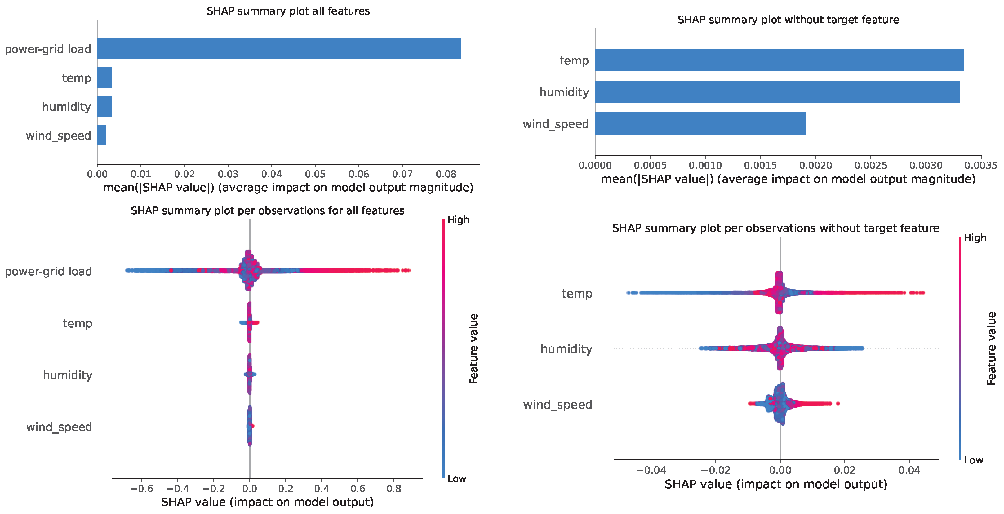
Best Model Interpretation Using Explainable AI

The possibility to explain the behavior exhibited by an ML model is vital to comprehend the process that is modeled and the obtained results. In order to explain the LSTM model that achieved the best level of performance on the power load dataset, the advanced explainable AI method Shapley additive explanations (SHAP) was employed. The SHAP procedure successfully evades the balancing betwixt the accuracy and the possibility to interpret the results, by providing a straightforward and relevant interpretation of the obtained LSTM predictions. SHAP relies on Shapley values, inspired by game theory, that represent the feature importance metric, providing an insight into what attributes have the largest influence on the predictions [74].

Simply said, Shapley values denote a set of distributed payouts between players that work together (representing the features) with respect to their contributions to the joint payout (denoting the prediction). Consequently, the SHAP method allocates to each feature an additional metric—the importance, that measures the contribution of that feature to the specific prediction, by calculating the impact of the model’s prediction in comparison to the prediction if that particular feature was set to a baseline value.

The best-performing LSTM model obtained from experiments (LSTM-FA) was taken and Shapley values were calculated. To observe the influence of each predictor on the final output in the testing set, SHAP summary plots for all features with and without the target variable, which was also used as predictor, were created and are shown in Figure 7. Summary plots in the form of bars (first row in the figure) represent the relative importance of each feature, calculated by taking the average absolute value of the SHAP values. Plots shown in the second row of the figure depict the influence that each observation has on the target variable (power-grid load).

From Figure 7, some important conclusions can be observed. First, the feature that has the most relative importance on the target is the power-grid load in the past period, in this case in the previous h. Secondly, the second most influential predictor is the temperature and, from the summary plots per each observation, it can be clearly noted that with the increase of temperature for most observations, the power-grid load is also increasing. This implication is logical because it is generally hot in Spain and people are using air conditioning systems for cooling that use a lot of electricity. Similar conclusions can be made for humidity and wind speed predictors on the total power-grid load (energy consumption).

5. Conclusions

Some of the most recent DL architectures for energy modeling, in general, are reviewed, with an emphasis on energy load prediction. Although there exist recent shallow ML approaches for energy forecasting, the supremacy of the DL-based models is generally acknowledged. The models are assessed from several facets, and one of them refers to whether hyperparameter tuning was used or not in previous works. When not specifically mentioned whether the hyperparameters were tuned via a specific method and their values were simply provided, it is assumed that manual tuning was performed.

As many of the recent research works made in this area do not use any dedicated tool or method for parameter tuning, a straightforward experiment was assembled herein that evaluates the necessity and adequacy of employing a specific tool for this task, e.g., a metaheuristic. As a counterpart, a grid search is used for tuning the same hyperparameters. A simple LSTM architecture to allow numerous simulations in a relatively short time was used. The overall results indicate that FA led to the best results out of the entire set of used heuristics, although the differences in the outputs are very small. Nevertheless, the results obtained when using any of the six metaheuristics for parameter tuning led to results notably better than when grid search was used for the same purpose. While it is true that DL is rarely a fast procedure, it is shown that even with an economical metaheuristic (e.g., a population of only four individuals evolved over five iterations), the results are improved to a great extent and, when possible, the integration of such supplementary mechanism pays off.

The goal of the current experiment was not to propose the most appropriate model for the problem at hand, but rather to demonstrate that hyperparameter tuning via metaheuristics leads to considerably better results. More complex DL approaches, such as bidirectional LSTM (BiLSTM) or gated recurrent units (GRUs), would probably improve the results, especially if properly tuned. Still, the results that are presented in the current work can be used for comparative studies in the future, as obtained from baseline approaches. We conclude by recommending the use of metaheuristics for the hyperparameters of the DL models since these generally lead to better-tailored models and, consequently, to improved results.

References

1. World Population to Reach 8 Billion on 15 November 2022. Available online: https://www.un.org/en/desa/world-population-reach-8-billion-15-november-2022 (accessed on 15 November 2022).
2. Shah, I.; Iftikhar, H.; Ali, S. Modeling and Forecasting Medium-Term Electricity Consumption Using Component Estimation Technique. Forecasting 2020, 2, 163–179. [Google Scholar] [CrossRef]
3. Chinnaraji, R.; Ragupathy, P. Accurate electricity consumption prediction using enhanced long short-term memory. IET Commun. 2022, 16, 830–844. [Google Scholar] [CrossRef]
4. Jaaz, Z.A.; Rusli, M.E.; Rahmat, N.A.; Khudhair, I.Y.; Al Barazanchi, I.; Mehdy, H.S. A Review on Energy-Efficient Smart Home Load Forecasting Techniques. In Proceedings of the 2021 8th International Conference on Electrical Engineering, Computer Science and Informatics (EECSI), Semarang, Indonesia, 20–21 October 2021; pp. 233–240. [Google Scholar] [CrossRef]
5. Reddy, S.; Akashdeep, S.; Harshvardhan, R.; Kamath, S. Stacking Deep learning and Machine learning models for short-term energy consumption forecasting. Adv. Eng. Inform. 2022, 52, 101542. [Google Scholar] [CrossRef]
6. Salam, A.; El Hibaoui, A. Energy consumption prediction model with deep inception residual network inspiration and LSTM. Math. Comput. Simul. 2021, 190, 97–109. [Google Scholar] [CrossRef]
7. Mahanta Barua, A.; Goswami, P. A Survey on Electric Power Consumption Prediction Techniques. Int. J. Eng. Res. Technol. 2020, 13, 2568. [Google Scholar] [CrossRef]
8. Liang, Y.; Niu, D.; Hong, W.C. Short term load forecasting based on feature extraction and improved general regression neural network model. Energy 2019, 166, 653–663. [Google Scholar] [CrossRef]
9. Xu, L.; Hou, L.; Zhu, Z.; Li, Y.; Liu, J.; Lei, T.; Wu, X. Mid-term prediction of electrical energy consumption for crude oil pipelines using a hybrid algorithm of support vector machine and genetic algorithm. Energy 2021, 222, 119955. [Google Scholar] [CrossRef]
10. Gupta, A.; Chawla, M.; Tiwari, N. Electricity Power Consumption Forecasting Techniques: A Survey; SSRN: Rochester, NY, USA, 2022. [Google Scholar] [CrossRef]
11. Torres, J.F.; Hadjout, D.; Sebaa, A.; Martínez-Álvarez, F.; Troncoso, A. Deep learning for time series forecasting: A survey. Big Data 2021, 9, 3–21. [Google Scholar] [CrossRef]
12. Akiba, T.; Sano, S.; Yanase, T.; Ohta, T.; Koyama, M. Optuna: A Next-generation Hyperparameter Optimization Framework. In Proceedings of the 25rd ACM SIGKDD International Conference on Knowledge Discovery and Data Mining, Anchorage, AK, USA, 4–8 August 2019. [Google Scholar]
13. Mashlakov, A.; Kuronen, T.; Lensu, L.; Kaarna, A.; Honkapuro, S. Assessing the performance of deep learning models for multivariate probabilistic energy forecasting. Appl. Energy 2021, 285, 116405. [Google Scholar] [CrossRef]
14. Wiese, F.; Schlecht, I.; Bunke, W.D.; Gerbaulet, C.; Hirth, L.; Jahn, M.; Kunz, F.; Lorenz, C.; Mühlenpfordt, J.; Reimann, J.; et al. Open Power System Data—Frictionless data for electricity system modelling. Appl. Energy 2019, 236, 401–409. [Google Scholar] [CrossRef]
15. Kim, T.Y.; Cho, S.B. Predicting residential energy consumption using CNN-LSTM neural networks. Energy 2019, 182, 72–81. [Google Scholar] [CrossRef]
16. Hebrail, G.; Berard, A. Individual Household Electric Power Consumption Data Set; UCI Machine Learning Repository: Irvine, CA, USA, 2012. [Google Scholar]
17. Somu, N.; Raman, M.R.G.; Ramamritham, K. A hybrid model for building energy consumption forecasting using long short term memory networks. Appl. Energy 2020, 261, 114131. [Google Scholar] [CrossRef]
18. Dong, H.; Zhu, J.; Li, S.; Wu, W.; Zhu, H.; Fan, J. Short-term residential household reactive power forecasting considering active power demand via deep Transformer sequence-to-sequence networks. Appl. Energy 2023, 329, 120281. [Google Scholar] [CrossRef]
19. Meinrenken, C.J.; Rauschkolb, N.; Abrol, S.; Chakrabarty, T.; Decalf, V.C.; Hidey, C.; McKeown, K.; Mehmani, A.; Modi, V.; Culligan, P.J. MFRED, 10 s interval real and reactive power for groups of 390 US apartments of varying size and vintage. Sci. Data 2020, 7, 375. [Google Scholar] [CrossRef]
20. Hadjout, D.; Torres, J.; Troncoso, A.; Sebaa, A.; Martínez-Álvarez, F. Electricity consumption forecasting based on ensemble deep learning with application to the Algerian market. Energy 2022, 243, 123060. [Google Scholar] [CrossRef]
21. Lv, R.; Yuan, Z.; Lei, B.; Zheng, J.; Luo, X. Building thermal load prediction using deep learning method considering time-shifting correlation in feature variables. J. Build. Eng. 2022, 61, 105316. [Google Scholar] [CrossRef]
22. Ahajjam, M.A.; Bonilla Licea, D.; Ghogho, M.; Kobbane, A. Experimental investigation of variational mode decomposition and deep learning for short-term multi-horizon residential electric load forecasting. Appl. Energy 2022, 326, 119963. [Google Scholar] [CrossRef]
23. Ahajjam, M.A.; Bonilla Licea, D.; Essayeh, C.; Ghogho, M.; Kobbane, A. MORED: A Moroccan Buildings’ Electricity Consumption Dataset. Energies 2020, 13, 6737. [Google Scholar] [CrossRef]
24. Gao, R.; Du, L.; Suganthan, P.N.; Zhou, Q.; Yuen, K.F. Random vector functional link neural network based ensemble deep learning for short-term load forecasting. Expert Syst. Appl. 2022, 206, 117784. [Google Scholar] [CrossRef]
25. Alotaibi, M.A. Machine Learning Approach for Short-Term Load Forecasting Using Deep Neural Network. Energies 2022, 15, 6261. [Google Scholar] [CrossRef]
26. Aouad, M.; Hajj, H.; Shaban, K.; Jabr, R.A.; El-Hajj, W. A CNN-Sequence-to-Sequence network with attention for residential short-term load forecasting. Electr. Power Syst. Res. 2022, 211, 108152. [Google Scholar] [CrossRef]
27. Ibrahim, B.; Rabelo, L.; Gutierrez-Franco, E.; Clavijo-Buritica, N. Machine Learning for Short-Term Load Forecasting in Smart Grids. Energies 2022, 15, 8079. [Google Scholar] [CrossRef]
28. Saha, B.; Ahmed, K.F.; Saha, S.; Islam, M.T. Short-Term Electrical Load Forecasting via Deep Learning Algorithms to Mitigate the Impact of COVID-19 Pandemic on Power Demand. In Proceedings of the 2021 International Conference on Automation, Control and Mechatronics for Industry 4.0 (ACMI), Rajshahi, Bangladesh, 8–9 July 2021; pp. 1–6. [Google Scholar] [CrossRef]
29. Li, X.; Wang, Y.; Ma, G.; Chen, X.; Shen, Q.; Yang, B. Electric load forecasting based on Long-Short-Term-Memory network via simplex optimizer during COVID-19. Energy Rep. 2022, 8, 1–12. [Google Scholar] [CrossRef]
30. Tudose, A.M.; Picioroaga, I.I.; Sidea, D.O.; Bulac, C.; Boicea, V.A. Short-Term Load Forecasting Using Convolutional Neural Networks in COVID-19 Context: The Romanian Case Study. Energies 2021, 14, 4046. [Google Scholar] [CrossRef]
31. Zhu, J.; Dong, H.; Zheng, W.; Li, S.; Huang, Y.; Xi, L. Review and prospect of data-driven techniques for load forecasting in integrated energy systems. Appl. Energy 2022, 321, 119269. [Google Scholar] [CrossRef]
32. Hourly Energy Demand Generation and Weather. Available online: https://www.kaggle.com/datasets/nicholasjhana/energy-consumption-generation-prices-and-weather (accessed on 21 November 2022).
33. Sherstinsky, A. Fundamentals of recurrent neural network (RNN) and long short-term memory (LSTM) network. Phys. D Nonlinear Phenom. 2020, 404, 132306. [Google Scholar] [CrossRef]
34. Stoean, C.; Paja, W.; Stoean, R.; Sandita, A. Deep architectures for long-term stock price prediction with a heuristic-based strategy for trading simulations. PLoS ONE 2019, 14, e0223593. [Google Scholar] [CrossRef] [Green Version]
35. Bukhari, A.H.; Raja, M.A.Z.; Sulaiman, M.; Islam, S.; Shoaib, M.; Kumam, P. Fractional neuro-sequential ARFIMA-LSTM for financial market forecasting. IEEE Access 2020, 8, 71326–71338. [Google Scholar] [CrossRef]
36. Sagheer, A.; Kotb, M. Time series forecasting of petroleum production using deep LSTM recurrent networks. Neurocomputing 2019, 323, 203–213. [Google Scholar] [CrossRef]
37. Stoean, C.; Stoean, R.; Atencia, M.; Abdar, M.; Velázquez-Pérez, L.; Khosravi, A.; Nahavandi, S.; Acharya, U.R.; Joya, G. Automated Detection of Presymptomatic Conditions in Spinocerebellar Ataxia Type 2 Using Monte Carlo Dropout and Deep Neural Network Techniques with Electrooculogram Signals. Sensors 2020, 20, 3032. [Google Scholar] [CrossRef]
38. Stoean, R.; Stoean, C.; Atencia, M.; Rodríguez-Labrada, R.; Joya, G. Ranking Information Extracted from Uncertainty Quantification of the Prediction of a Deep Learning Model on Medical Time Series Data. Mathematics 2020, 8, 1078. [Google Scholar] [CrossRef]
39. Shahid, F.; Zameer, A.; Muneeb, M. Predictions for COVID-19 with deep learning models of LSTM, GRU and Bi-LSTM. Chaos Solitons Fractals 2020, 140, 110212. [Google Scholar] [CrossRef] [PubMed]
40. Chimmula, V.K.R.; Zhang, L. Time series forecasting of COVID-19 transmission in Canada using LSTM networks. Chaos Solitons Fractals 2020, 135, 109864. [Google Scholar] [CrossRef] [PubMed]
41. Zivkovic, M.; Bacanin, N.; Venkatachalam, K.; Nayyar, A.; Djordjevic, A.; Strumberger, I.; Al-Turjman, F. COVID-19 cases prediction by using hybrid machine learning and beetle antennae search approach. Sustain. Cities Soc. 2021, 66, 102669. [Google Scholar] [CrossRef] [PubMed]
42. Zivkovic, M.; Venkatachalam, K.; Bacanin, N.; Djordjevic, A.; Antonijevic, M.; Strumberger, I.; Rashid, T.A. Hybrid Genetic Algorithm and Machine Learning Method for COVID-19 Cases Prediction. In Proceedings of the International Conference on Sustainable Expert Systems: ICSES 2020; Springer Nature: Berlin/Heidelberg, Germany, 2021; Volume 176, p. 169. [Google Scholar]
43. Bacanin, N.; Bezdan, T.; Tuba, E.; Strumberger, I.; Tuba, M.; Zivkovic, M. Task scheduling in cloud computing environment by grey wolf optimizer. In Proceedings of the 2019 27th Telecommunications Forum (TELFOR), Belgrade, Serbia, 26–27 November 2019; pp. 1–4. [Google Scholar]
44. Bezdan, T.; Zivkovic, M.; Tuba, E.; Strumberger, I.; Bacanin, N.; Tuba, M. Multi-objective Task Scheduling in Cloud Computing Environment by Hybridized Bat Algorithm. In Proceedings of the International Conference on Intelligent and Fuzzy Systems, Istanbul, Turkey, 21–23 July 2020; pp. 718–725. [Google Scholar]
45. Bezdan, T.; Zivkovic, M.; Antonijevic, M.; Zivkovic, T.; Bacanin, N. Enhanced Flower Pollination Algorithm for Task Scheduling in Cloud Computing Environment. In Machine Learning for Predictive Analysis; Springer: Berlin/Heidelberg, Germany, 2020; pp. 163–171. [Google Scholar]
46. Zivkovic, M.; Bezdan, T.; Strumberger, I.; Bacanin, N.; Venkatachalam, K. Improved Harris Hawks Optimization Algorithm for Workflow Scheduling Challenge in Cloud–Edge Environment. In Computer Networks, Big Data and IoT; Springer: Berlin/Heidelberg, Germany, 2021; pp. 87–102. [Google Scholar]
47. Zivkovic, M.; Bacanin, N.; Tuba, E.; Strumberger, I.; Bezdan, T.; Tuba, M. Wireless Sensor Networks Life Time Optimization Based on the Improved Firefly Algorithm. In Proceedings of the 2020 International Wireless Communications and Mobile Computing (IWCMC), Limassol, Cyprus, 15–19 June 2020; pp. 1176–1181. [Google Scholar]
48. Zivkovic, M.; Bacanin, N.; Zivkovic, T.; Strumberger, I.; Tuba, E.; Tuba, M. Enhanced Grey Wolf Algorithm for Energy Efficient Wireless Sensor Networks. In Proceedings of the 2020 Zooming Innovation in Consumer Technologies Conference (ZINC), Novi Sad, Serbia, 26–27 May 2020; pp. 87–92. [Google Scholar]
49. Bacanin, N.; Tuba, E.; Zivkovic, M.; Strumberger, I.; Tuba, M. Whale Optimization Algorithm with Exploratory Move for Wireless Sensor Networks Localization. In Proceedings of the International Conference on Hybrid Intelligent Systems, Bhopal, India, 10–12 December 2019; pp. 328–338. [Google Scholar]
50. Zivkovic, M.; Zivkovic, T.; Venkatachalam, K.; Bacanin, N. Enhanced Dragonfly Algorithm Adapted for Wireless Sensor Network Lifetime Optimization. In Data Intelligence and Cognitive Informatics; Springer: Berlin/Heidelberg, Germany, 2021; pp. 803–817. [Google Scholar]
51. Bezdan, T.; Cvetnic, D.; Gajic, L.; Zivkovic, M.; Strumberger, I.; Bacanin, N. Feature Selection by Firefly Algorithm with Improved Initialization Strategy. In Proceedings of the 7th Conference on the Engineering of Computer Based Systems, Novi Sad, Serbia, 26–27 May 2021; pp. 1–8. [Google Scholar]
52. Stoean, C. In Search of the Optimal Set of Indicators when Classifying Histopathological Images. In Proceedings of the 2016 18th International Symposium on Symbolic and Numeric Algorithms for Scientific Computing (SYNASC), Timisoara, Romania, 24–27 September 2016; pp. 449–455. [Google Scholar] [CrossRef]
53. Nadimi-Shahraki, M.H.; Zamani, H.; Mirjalili, S. Enhanced whale optimization algorithm for medical feature selection: A COVID-19 case study. Comput. Biol. Med. 2022, 148, 105858. [Google Scholar] [CrossRef] [PubMed]
54. Bezdan, T.; Zivkovic, M.; Tuba, E.; Strumberger, I.; Bacanin, N.; Tuba, M. Glioma Brain Tumor Grade Classification from MRI Using Convolutional Neural Networks Designed by Modified FA. In Proceedings of the International Conference on Intelligent and Fuzzy Systems, Istanbul, Turkey, 21–23 July 2020; pp. 955–963. [Google Scholar]
55. Postavaru, S.; Stoean, R.; Stoean, C.; Caparros, G.J. Adaptation of Deep Convolutional Neural Networks for Cancer Grading from Histopathological Images. In Proceedings of the Advances in Computational Intelligence, Cadiz, Spain, 14–16 June 2017; Rojas, I., Joya, G., Catala, A., Eds.; Springer International Publishing: Cham, Switzerland, 2017; pp. 38–49. [Google Scholar]
56. Zivkovic, M.; Bacanin, N.; Antonijevic, M.; Nikolic, B.; Kvascev, G.; Marjanovic, M.; Savanovic, N. Hybrid CNN and XGBoost Model Tuned by Modified Arithmetic Optimization Algorithm for COVID-19 Early Diagnostics from X-ray Images. Electronics 2022, 11, 3798. [Google Scholar] [CrossRef]
57. Strumberger, I.; Tuba, E.; Zivkovic, M.; Bacanin, N.; Beko, M.; Tuba, M. Dynamic search tree growth algorithm for global optimization. In Proceedings of the Doctoral Conference on Computing, Electrical and Industrial Systems, Costa de Caparica, Portugal, 8–10 May 2019; pp. 143–153. [Google Scholar]
58. Preuss, M.; Stoean, C.; Stoean, R. Niching Foundations: Basin Identification on Fixed-Property Generated Landscapes. In Proceedings of the 13th Annual Conference on Genetic and Evolutionary Computation, GECCO’11, Dublin, Ireland, 12–16 July 2011; Association for Computing Machinery: New York, NY, USA, 2011; pp. 837–844. [Google Scholar] [CrossRef]
59. Jovanovic, D.; Antonijevic, M.; Stankovic, M.; Zivkovic, M.; Tanaskovic, M.; Bacanin, N. Tuning Machine Learning Models Using a Group Search Firefly Algorithm for Credit Card Fraud Detection. Mathematics 2022, 10, 2272. [Google Scholar] [CrossRef]
60. Petrovic, A.; Bacanin, N.; Zivkovic, M.; Marjanovic, M.; Antonijevic, M.; Strumberger, I. The AdaBoost Approach Tuned by Firefly Metaheuristics for Fraud Detection. In Proceedings of the 2022 IEEE World Conference on Applied Intelligence and Computing (AIC), Sonbhadra, India, 17–19 June 2022; pp. 834–839. [Google Scholar]
61. Bacanin, N.; Sarac, M.; Budimirovic, N.; Zivkovic, M.; AlZubi, A.A.; Bashir, A.K. Smart wireless health care system using graph LSTM pollution prediction and dragonfly node localization. Sustain. Comput. Inform. Syst. 2022, 35, 100711. [Google Scholar] [CrossRef]
62. Bacanin, N.; Zivkovic, M.; Stoean, C.; Antonijevic, M.; Janicijevic, S.; Sarac, M.; Strumberger, I. Application of Natural Language Processing and Machine Learning Boosted with Swarm Intelligence for Spam Email Filtering. Mathematics 2022, 10, 4173. [Google Scholar] [CrossRef]
63. Stankovic, M.; Antonijevic, M.; Bacanin, N.; Zivkovic, M.; Tanaskovic, M.; Jovanovic, D. Feature Selection by Hybrid Artificial Bee Colony Algorithm for Intrusion Detection. In Proceedings of the 2022 International Conference on Edge Computing and Applications (ICECAA), Coimbatore, India, 21–23 September 2022; pp. 500–505. [Google Scholar]
64. Milosevic, S.; Bezdan, T.; Zivkovic, M.; Bacanin, N.; Strumberger, I.; Tuba, M. Feed-Forward Neural Network Training by Hybrid Bat Algorithm. In Proceedings of the Modelling and Development of Intelligent Systems: 7th International Conference, MDIS 2020, Sibiu, Romania, 22–24 October 2020; Revised Selected Papers 7. Springer International Publishing: Berlin/Heidelberg, Germany, 2021; pp. 52–66. [Google Scholar]
65. Gajic, L.; Cvetnic, D.; Zivkovic, M.; Bezdan, T.; Bacanin, N.; Milosevic, S. Multi-layer Perceptron Training Using Hybridized Bat Algorithm. In Computational Vision and Bio-Inspired Computing; Springer: Berlin/Heidelberg, Germany, 2021; pp. 689–705. [Google Scholar]
66. Bacanin, N.; Stoean, C.; Zivkovic, M.; Jovanovic, D.; Antonijevic, M.; Mladenovic, D. Multi-Swarm Algorithm for Extreme Learning Machine Optimization. Sensors 2022, 22, 4204. [Google Scholar] [CrossRef]
67. Jovanovic, L.; Jovanovic, D.; Bacanin, N.; Jovancai Stakic, A.; Antonijevic, M.; Magd, H.; Thirumalaisamy, R.; Zivkovic, M. Multi-Step Crude Oil Price Prediction Based on LSTM Approach Tuned by Salp Swarm Algorithm with Disputation Operator. Sustainability 2022, 14, 14616. [Google Scholar] [CrossRef]
68. Mirjalili, S. Genetic algorithm. In Evolutionary Algorithms and Neural Networks; Springer: Berlin/Heidelberg, Germany, 2019; pp. 43–55. [Google Scholar]
69. Kennedy, J.; Eberhart, R. Particle swarm optimization. In Proceedings of the ICNN’95-International Conference on Neural Networks, Perth, WA, Australia, 27 November–1 December 1995; Volume 4, pp. 1942–1948. [Google Scholar]
70. Karaboga, D.; Basturk, B. On the performance of artificial bee colony (ABC) algorithm. Appl. Soft Comput. 2008, 8, 687–697. [Google Scholar] [CrossRef]
71. Yang, X.S.; Slowik, A. Firefly algorithm. In Swarm Intelligence Algorithms; CRC Press: Boca Raton, FL, USA, 2020; pp. 163–174. [Google Scholar]
72. Yang, X.S. A new metaheuristic bat-inspired algorithm. In Nature Inspired Cooperative Strategies for Optimization (NICSO 2010); Springer: Berlin/Heidelberg, Germany, 2010; pp. 65–74. [Google Scholar]
73. Mirjalili, S. SCA: A Sine Cosine Algorithm for Solving Optimization Problems. Knowl.-Based Syst. 2016, 96, 120–133. [Google Scholar] [CrossRef]
74. Lundberg, S.M.; Lee, S.I. A unified approach to interpreting model predictions. In Proceedings of the Advances in Neural Information Processing Systems 30 (NIPS 2017), Long Beach, CA, USA, 4–9 December 2017; Volume 30. [Google Scholar]
Figure 2. The visual representation of the used dataset. The training, validation, and test sets are highlighted using different colors.
Energies 16 01434 g002
Figure 3. Visualizations of the executed LSTM experiments for all 6 algorithms in terms of convergence, box plot, violin diagrams, and swarm diversity diagrams for the objective function (MSE).
Energies 16 01434 g003
Figure 4. Visualizations of the executed LSTM experiments for all 6 algorithms in terms of convergence, box plot, violin diagrams, and swarm diversity diagrams for the R 2 indicator.
Energies 16 01434 g004
Figure 5. Visualizations of the kernel distribution estimation plots for both the objective function (MSE) and R2.
Energies 16 01434 g005
Figure 6. The best predictions by the LSTM model determined by each observed metaheuristic.
Energies 16 01434 g006
Figure 7. SHAP summary plots for the testing set based on the LSTM-FA tuned model.
Energies 16 01434 g007