Classification of Wear State for a Positive Displacement Pump Using Deep Machine Learning ^†

Abstract

Hydraulic power systems are commonly used in heavy industry (usually highly energy-intensive) and are often associated with high power losses. Designing a suitable system to allow an early assessment of the wear conditions of components in a hydraulic system (e.g., an axial piston pump) can effectively contribute to reducing energy losses during use. This paper presents the application of a deep machine learning system to determine the efficiency state of a multi-piston positive displacement pump. Such pumps are significant in high-power hydraulic systems. The correct operation of the entire hydraulic system often depends on its proper functioning. The wear and tear of individual pump components usually leads to a decrease in the pump’s operating pressure and volumetric losses, subsequently resulting in a decrease in overall pump efficiency and increases in vibration and pump noise. This in turn leads to an increase in energy losses throughout the hydraulic system, which releases excess heat. Typical failures of the discussed pumps and their causes are described after reviewing current research work using deep machine learning. Next, the test bench on which the diagnostic experiment was conducted and the selected operating signals that were recorded are described. The measured signals were subjected to a time–frequency analysis, and their features, calculated in terms of the time and frequency domains, underwent a significance ranking using the minimum redundancy maximum relevance (MRMR) algorithm. The next step was to design a neural network structure to classify the wear state of the pump and to test and evaluate the effectiveness of the network’s recognition of the pump’s condition. The whole study was summarized with conclusions.

1. Introduction

A positive displacement pump is one of the most important components of hydrostatic systems. A special place in the construction of such systems is occupied by axial piston pumps, which, due to the possibility of working with high and very high pressures (higher than other pump designs such as gear pumps) and the possibility of working with a wide range of regulators and adjusters (e.g., regulators of power, pressure, and flow), are regarded as the main pumps of such drives [1,2,3].

The possibility of assessing the state of wear of an operating pump is not only an interesting research issue but also leads to the elimination of the uncontrolled downtime of hydrostatic systems due to their failures.

Maintaining a hydraulic system in good working order requires constant supervision of both its basic hydraulic parameters (pressures and flow rates) and additional operating signals associated with the working of such a system, including vibration signals, temperature changes, and the purity class of the operating medium, that are often present in these types of systems. This usually requires retrofitting a system in operation with additional measuring transducers found in their typical locations. The signals measured with the transducers provide diagnostic information that is used to develop a system that monitors the condition of the hydraulic system.

In current research work and the systems already in use to control the performance of entire hydraulic systems (as well as individual components), it is possible to distinguish three main approaches [4,5]:

✓

Diagnostic systems for hydraulics (components) based on the developed model of the diagnosed system

Such a solution was used in specific papers [6,7] to detect malfunctions in axial displacement pumps and consisted of assessing the resulting leaks in the piston–cylinder pairs of these pumps using an extended Kalman filter [8] as a condition observer. The detection of hydraulic cylinder piston seal leaks by means of an adaptive Kalman filter was suggested in [9]. An interesting application of a sliding observer with modified (adaptable) gain in an electrohydraulic positioning system diagnosis was presented in [10].

✓

Diagnostic systems for hydraulic systems (components) based on signal analysis

Wavelet analysis and the Hilbert–Huang transform as well as well-known methods of the time–frequency analysis of signals are commonly used in these types of systems [11].

The use of the wavelet transform to monitor the condition of hydraulic cylinder seals, the failure of which lead to leaks outside (and inside) the cylinder, was described in [12]. Moreover, the issue of leakage inside the actuator and its detection using the Hilbert–Huang transform to analyze the measured signals was described in [13]. Another example of the use of signal analysis in the diagnosis of a common malfunction of multi-piston pumps, i.e., damage to the piston rod feet, is the use of adaptive morphological analysis [14].

✓

Diagnostic systems for hydraulics (components) using the so-called intelligent fault identification

A lot of research on intelligent fault identification has been conducted and successfully applied to the diagnostics of hydraulic systems [15,16,17,18]. This type of system is based on using machine learning algorithms and deep machine learning [19].

In [20], the authors describe the use of the support vector machine (SVM) algorithm in the classification of the degree of wear of hydraulic brakes. Another example of the use of machine learning methods is the use of the extreme learning machine (ELM) classifier described in [21] to assess the wear condition of the piston feet of multi-piston pumps.

The application of deep machine learning in monitoring the performance of hydraulic system components was described using the example of employing such a system in the diagnostics of a two-stage hydraulic distributor [22]. The article presented the possibility of classifying the damage of such a distributor based on the newly developed multi-stage classifier using the Dezert–Smarandache theory. The proposed method had a high efficiency (98.1%) and was compared with other systems utilizing convolutional neural networks (CNNs) and long short-term memory network (LSTM) recurrent networks as classifiers. The use of deep machine learning to detect cavitation phenomena in centrifugal pumps’ suction ports based on the pressure signal measurements in their discharge ports was described in [23].

Articles presented the application of deep machine learning using DBNs (deep belief networks) in fault classification in axial piston pumps [24]. An experimental study was carried out to detect and classify the four most typical axial piston pump faults. The classification accuracy rate was 97.40%, which confirmed the feasibility and effectiveness of detecting multiple faults in axial piston pumps with the use of DBNs (deep belief networks).

From the examples of the diagnosis of hydrostatic components and systems presented above, it can be seen that the diagnosis of these systems is usually conducted under stationary operating conditions, i.e., at a stabilized working fluid temperature. In the authors’ opinion, this approach places a significant limitation on the assessment of the degree of wear of the components being tested. Therefore, to assess the wear condition of a multi-piston pump, it was proposed to analyze the signals measured both in stationary and non-stationary conditions of its operation [5].

A large proportion of the work devoted to the subject of the diagnosis of malfunctions in positive displacement pumps is based on the use of pre-prepared failures of pump components, which are then incorporated into their design. With this approach, the damage development cannot be fully pictured and is only an approximation. The authors of an article used a different approach [5] based on obtaining the wear of elements of the tested pump in a natural way based on its lengthy operation under the assumed load at a lower oil-cleanliness class. Except for achieving the natural wear of the pump components, the presented method gives the opportunity to control the development of damage and associated symptoms.

In this article, the authors present the use of deep machine learning [25,26] to classify the wear state of a multi-piston positive displacement pump. In engineering applications, deep machine learning systems are valued due to numerous advantages, among which is the ability to develop a system with good classification accuracy utilizing a reasonable amount of learning data and short learning times for the developed diagnostic models. From the outset [5], it was assumed that the learning system would rest upon measures (features) derived from vibration signals recorded at characteristic locations in the pump body and additional signals from static and dynamic pressure transducers fitted in the discharge port obtained as a result of a passive diagnostic experiment. The selection of measures calculated from the measured signals and the subsequent ranking of their relevance in the classification of the pump’s wear state was completed using the minimum redundancy maximum relevance (MRMR) algorithm [27].

The original nature of this paper is the result of the following methods:

-

The application of the minimum redundancy maximum relevance (MRMR) algorithm in ranking the features determined from the measured signals;

-

Designing a neural classifier of the pump wear state based on the ranked features of the measured signals;

-

Preparing and carrying out a test experiment to naturally obtain the wear and tear of the pump components based on the lengthy operation of the pump at a lower oil grade;

-

The use of signals measured across the entire operating range of the pump (i.e., when in stationary and non-stationary operating conditions) to assess the wear state of the tested pump.

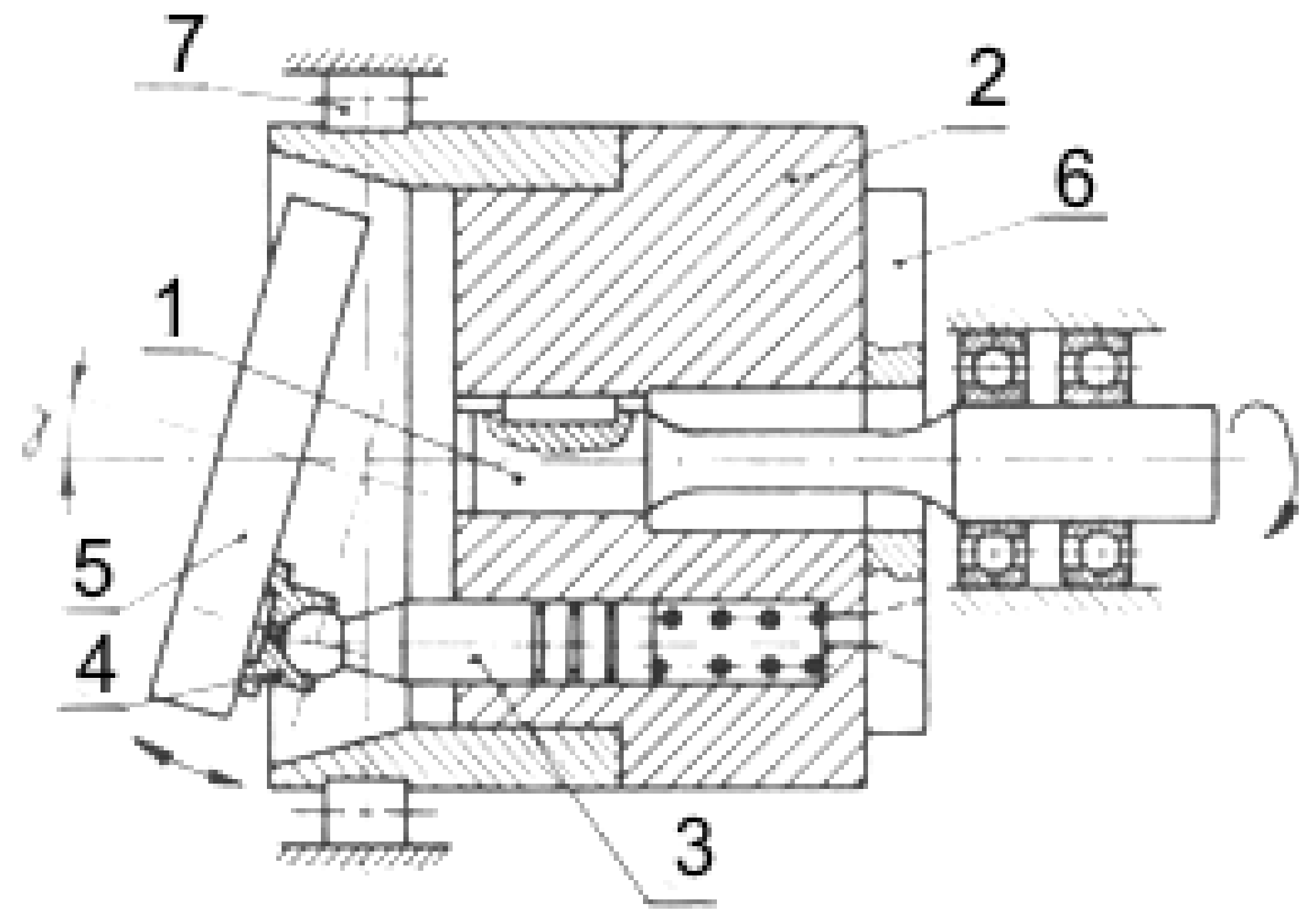
2. Object of the Study

An axial multi-piston pump with a swashplate (the simplified design scheme of which is shown in Figure 1) was the object of the research. This type of design is characterized by the rotor (2) and piston assembly (3) mounted coaxially on the drive shaft (1). The feet (4) of the pistons cooperating with a stationary disc (5) pivoted at an angle (γ) with regard to the axis of the pump rotor.

The pistons, together with the rotor, perform a rotary motion, and, sliding on the surface of the stationary swashplate, their feet (4) further force a progressive-return motion in the rotor cylinders. The rotor slides on a stationary valve plate (6) in which the pump’s suction and discharge ports are provided. The wear and tear of the elements within the positive displacement pumps are determined by the forces that occur during the cooperation of various elements forming kinematic pairs (e.g., piston–cylinder, valve plate–rotor, and piston foot–swashplate) and the inadequate operating conditions of the pumps, e.g., exceeding the nominal working pressure, low viscosity of the operating medium, or its insufficient filtration. The type of wear that occurs most typically in positive displacement pump components is abrasive wear [29,30]. This type of wear appears in all elements of the pump experiencing relative motion and contact between them. In the case of the analyzed multi-piston pump designs, this applies, for instance, to the surface of its swashplate. Swashplate wear is associated with the phenomenon of a deepening elliptical depression on its surface, caused by a permanent or partial loss of hydrostatic support between the surface of the disc and the surface of the piston foot sliding on it. The lack of hydrostatic support of the piston foot–swashplate pair can be a result of the excessive operating pressure of the pump at the same time as its operating medium has low viscosity. This leads to the disappearance of the lubricating layer between the moving components (the disappearance of hydrostatic support) and a shift of the components working together into the mixed or dry friction range.

The progressive wear of pump components can be tracked using conventional diagnostic methods, which are based on time and time–frequency analyses of the measured signals [11].

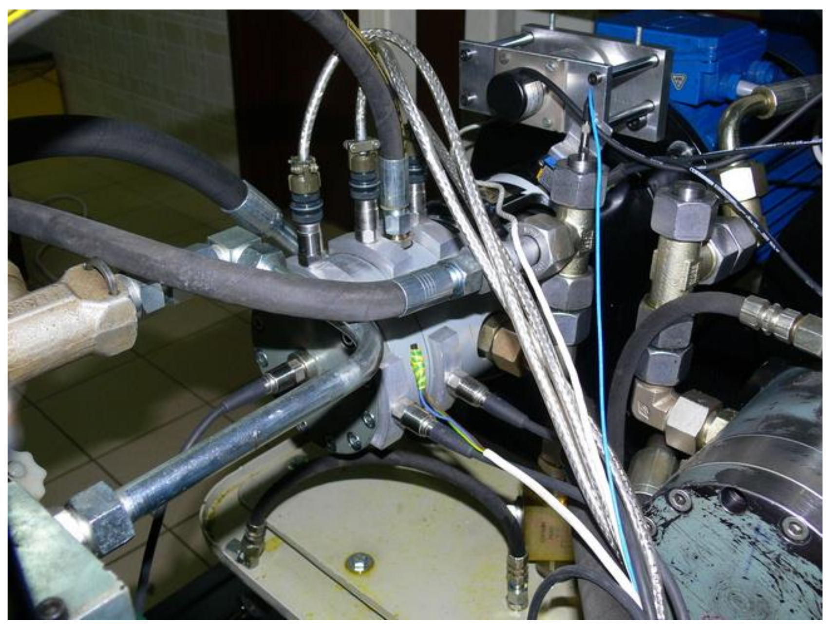
3. Course of the Study

Studies devoted to the subject of wear development in the multi-piston pump components were conducted on a laboratory bench specially built for this purpose. One of the main objectives of this study was to achieve the wear of the pump components in a natural way; therefore, the tests lasted many hours and were conducted in the actual operating conditions of the pump. During the study experiment, the live recording of diagnostic signals was carried out with the following assembled measuring transducers:

• A static pressure transducer;
• A dynamic pressure transducer;
• A pump body vibration acceleration transducer.

Measurements of vibrating body acceleration were made for three measurement axes (X, Y, and Z) after mounting transducers on the pump body near the swashplate, rotor, and valve plate (Figure 2).

The pressures (static and dynamic) were measured in the pump’s discharge line directly at its outlet. The sampling frequency of the measured signals equaled 50 kHz. A simplified diagram of the test bench is shown in Figure 3. Taking advantage of the fact that during the measurements of the signals the pump shaft rotation marker signal was also measured, each of the recorded signals underwent division according to this signal. In the case of the pump operating at nominal speed (n = 1500 rpm), 25 splits were obtained from a signal of 1 s. This provided signal matrices with a length of one rotation (i.e., with a duration of: 0.04 s). One-second signals were recorded with fifteen-minute intervals between the measurements. Under a static load, the experiment included 10 h of pump operation per day (the whole experiment took about a week).

The operating status of the pump was supervised by measuring the change in static pressure at its output. Comparing the pressure values (for individual measurements) day by day, it was assumed that if the permissible pressure drop at the outlet of the pump reached a value of up to 10% of the value of the constant pressure of its load (this pressure was 70 bar), the tested pump remained operational (classifier: pump in working order). A further increase in the pressure drop at the pump outlet (up to 20% from the initial pressure) was classified as a near end-of-life condition of the pump (classifier: end of life). If the pressure drop at the pump outlet exceeded 20% of its initial value, the pump was treated as worn out (classifier: worn-out pump). A total of 441 waveforms of the measured signals (pump body vibration, static pressure, and dynamic pressure) were recorded, out of which 294 (147 each) constituted signals measured for an operational pump (classifier: pump in working order) or a pump in the transition condition (classifier: end of life). The last 147 runs were obtained in the operation process of a worn-out pump (classifier: worn-out pump). The next step in preparing the data for the pump performance status classification system was to divide them into data used in the learning process of the neural network and data meant for its subsequent testing and validation. It was assumed that a total of 30% of the general data would be used for validation and testing the correctness of the resulting classifier. The rest of the data (i.e., 70% of the general data) would be used in the process of network learning. The data thus prepared were loaded into the workspace of the Matlab package [31,32], where their further analysis was carried out, consisting of the following steps:

• The selection and calculation of appropriate signal features;
• The ranking of the calculated features with regard to the information they contained;
• Designing the structure of a neural network in a classifier system;
• Evaluating the effectiveness of the designed network in the classification of the wear state of the studied pump.

Selection of Classification System Features

Another critical issue in the classification system construction was selecting signal features on which the system would rely. The features of signals in the time domain, as well as the frequency domain, were identified for each of the obtained pump body vibration signal matrices [22,33]. The same was performed to analyze the signals from the static and dynamic pressure transducers fitted in the pump discharge port.

When the temporal characteristics of the measured signals were determined, their variability and the amount of information they contained were determined. Statistical measures of location, concentration, and variability were used. A summary of the mathematical relationships (with their descriptions), according to which the characteristics of the measured signals were calculated, is included in table in the next section.

The following were taken as frequency measures commonly used to describe signals in the frequency domain: the maximum value of the power spectral density (PSD) and the frequency value at which the amplitude of the PSD reached its maximum.

A total of 84 features were calculated from the measured signals, 66 of which were features derived from vibration signals, and 22 of which were obtained from measured pressures (static and dynamic). The calculated features of the signals (vibration and pressure) were sorted in tables, the last columns of which presented the classes (labels) of the pump’s operating status, i.e., pump in working order, end of life, and worn-out pump.

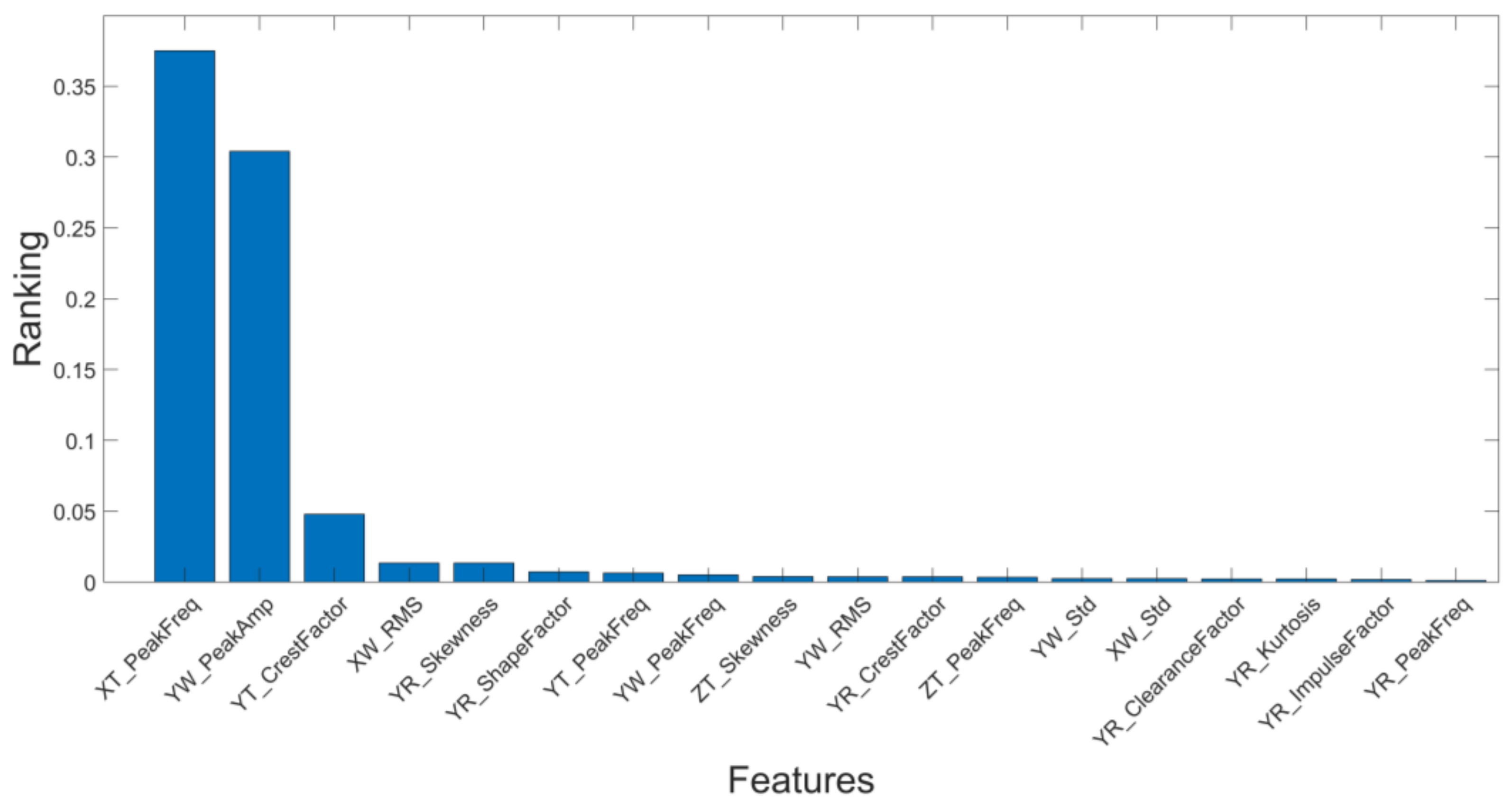
4. Significance Ranking of Signal Features

The calculated characteristics of the signals (

Table 1. List of features of the measured signals.

No.	Expression:	Feature:	Description:
1	$\stackrel{̲}{\mathrm{x}}=\frac{1}{\mathrm{n}}{\displaystyle \sum _{\mathrm{i}=1}^{\mathrm{n}}}{\mathrm{x}}_{\mathrm{i}}$	Mean	sum of all data divided by the number of data
2	$\mathsf{\delta }=\sqrt{{\mathsf{\delta }}^2}$ where ${\mathsf{\delta }}^2=\frac{1}{\mathrm{n}-1}{\displaystyle \sum _{\mathrm{i}=1}^{\mathrm{n}}}{\left({\mathrm{x}}_{\mathrm{i}}-\stackrel{̲}{\mathrm{x}}\right)}^2$	Standard deviation	square root of variance; the variance was estimated using a consistent and unbiased estimator
3	${\mathrm{x}}_{\mathrm{RMS}}=\sqrt{\frac{1}{\mathrm{n}}{\displaystyle \sum _{\mathrm{i}=1}^{\mathrm{n}}}{\mathrm{x}}_{\mathrm{i}}{}^2}$	Root mean square	square root of the arithmetic mean of the data squared
4	${\mathrm{x}}_{\mathrm{kurt}}=\frac{\frac{1}{\mathrm{n}}{\sum }_{\mathrm{i}=1}^{\mathrm{n}}{\left({\mathrm{x}}_{\mathrm{i}}-\stackrel{̲}{\mathrm{x}}\right)}^4}{{\mathsf{\delta }}^4}$	Kurtosis	measure of the shape of feature distribution
5	${\mathrm{x}}_{\mathrm{skw}}=\frac{\frac{1}{\mathrm{n}}{\sum }_{\mathrm{i}=1}^{\mathrm{n}}{\left({\mathrm{x}}_{\mathrm{i}}-\stackrel{̲}{\mathrm{x}}\right)}^3}{{\mathsf{\delta }}^3}$	Skewness	defines the degree to which the distribution differs from the normal distribution
6	${\mathrm{x}}_{\mathrm{sf}}=\frac{{\mathrm{x}}_{\mathrm{RMS}}}{\frac{1}{\mathrm{n}}{\sum }_{\mathrm{i}=1}^{\mathrm{n}}\left|{\mathrm{x}}_{\mathrm{i}}\right|}$	Shape factor	root mean square of the signal divided by the mean value of the signal
7	${\mathrm{x}}_{\mathrm{if}}=\frac{\max \left(\left|{\mathrm{x}}_{\mathrm{i}}\right|\right)}{\frac{1}{\mathrm{n}}{\sum }_{\mathrm{i}=1}^{\mathrm{n}}\left|{\mathrm{x}}_{\mathrm{i}}\right|}$	Impulse Factor	maximum absolute value of the signal divided by the mean absolute value of the signal
8	${\mathrm{x}}_{\mathrm{crest}}=\frac{\max \left(\left|{\mathrm{x}}_{\mathrm{i}}\right|\right)}{{\mathrm{x}}_{\mathrm{RMS}}}$	Crest Factor	maximum absolute value in the data divided by the root mean square of the data
9	${\mathrm{x}}_{\mathrm{clear}}=\frac{\max \left(\left|{\mathrm{x}}_{\mathrm{i}}\right|\right)}{{\left(\frac{1}{\mathrm{n}}{\sum }_{\mathrm{i}=1}^{\mathrm{n}}\sqrt{\left|{\mathrm{x}}_{\mathrm{i}}\right|}\right)}^2}$	Clearance Factor	maximum absolute value of the signal divided by the square root of the signal amplitude
10	max PSD	Peak amplitude of PSD	maximum value of the power spectral density
11	max Freq.	Peak frequency of PSD	frequency of the maximum value of power spectral density
xi—i-th measurement data point, n—total number of data in the measurement

) were carriers of information about the wear status of the monitored pump. As a general perception, the more information, the better the discriminatory power of the method used to classify sets of varying characteristics [34,35]. In theory, the number of calculated signal features (the input data for the classifier) is infinite, but the actual aim was to obtain the smallest number of features that provides a good description of the studied object’s properties. This was conducive to obtaining a compact model with a good fit in this article. The authors assumed that the five most relevant features would be selected to determine the wear state of the analyzed pump.

In order to improve the performance of the practical classifiers, it was necessary to remove correlated or irrelevant features, which led to a reduction in the dimensionality of the feature matrix and saved computational effort in developing the classifier models [36].

In this article, the minimum redundancy maximum relevance (MRMR) algorithm was used as a method for ranking the relevance of the calculated features.

A discussion of the feature relevance ranking algorithm is presented below.

Application of the Minimum Redundancy Maximum Relevance (MRMR) Algorithm in Ranking Calculated Features of Measured Signals

Optimizing the selection of features suitable for evaluating the wear rate of a multi-piston pump was carried out with the use of the minimum redundancy maximum relevance (MRMR) algorithm [27]. This algorithm identified the optimal—given a pump state classification (y)—set (S) of features x and z that maximized their applicability (V_S) and simultaneously minimized redundancy (W_S). The algorithm relied on the pairwise computed mutual information (I(x, z)) of features and the mutual information of features and pump condition (I(x, y)).

$$V_{\mathrm{s}}=\frac{1}{\left|S\right|}{\displaystyle \sum }_{x\in S}I\left(x,y\right)$$

(1)

$$W_{\mathrm{s}}=\frac{1}{{\left|S\right|}^2}{\displaystyle \sum }_{x,z\in S}I\left(x,z\right)$$

(2)

where:

V_s—applicability of features from set S;

W_s—redundancy of features from set S;

$\left|S\right|$—number of features in set S;

I(x, y)—calculated value of the mutual information of features x and y for the condition of the pump;

I(x, z)—calculated value of the mutual information of features x and z from set S.

The mutual information value (3) of features x and z in set S was calculated according to their joint probability distribution (p(x, y)) and the separate probability distributions (p(x) and p(y)) of the variables x and y by means of the adaptive algorithm described in [37]. In the same way, the mutual information value (I(x, y)) of the x features and the y state of the pump were calculated.

$$I\left(x, y\right)={\displaystyle \sum }_{i, j}p\left(x_i,y_j\right)·\log \frac{p\left(x_i,y_j\right)}{p\left(x_i\right)p\left(y_j\right)}$$

(3)

where:

p(x, y)—joint probabilistic distribution of feature x and state y;

p(x)—probability distribution of feature x;

p(y)—probability distribution of feature y.

Finding the optimal set (S) of features (from the full set (Ω) of all 62 calculated features from vibration signals and 22 features calculated on the basis of pressure signals) that minimized their redundancy and, at the same time, maximized their applicability required an algorithm that calculated the value of the mutual information coefficient (MIQ_X) (the quotient of a feature’s applicability to its redundancy). Feature classification rested upon the selection of those characterized by the largest MIQ_X coefficient values (practically, larger than the assumed cut-off value).

$$\begin{array}{c}max\\ x\in S^c\end{array}{\mathrm{MIQ}}_{\mathrm{X}}=\begin{array}{c}max\\ x\in S^c\end{array}\frac{I\left(x,y\right)}{\frac{1}{\left|S\right|}{\sum }_{z\in S}I\left(x,z\right)}$$

(4)

The significance rankings of the features calculated separately from vibration signal measurements and pressure signal measurements are graphically shown in Figure 4 (for vibration signals) and Figure 5 (for pressure signals).

Among the 62 features that were obtained from the pump body vibration measurements, the 5 most relevant features (i.e., the 3 features with calculated MIQ_X coefficient values greater than 0.05 and the next 2 highest-ranked coefficients) were chosen to evaluate the wear state of the pump. The features that satisfied the foregoing condition are listed in

Table 2. Fundamental features of vibration signals.

Feature	MIQX Coefficient Value
XT_PeakFreq	0.37
YW_PeakAmp	0.31
YT_CreastFactor	0.05
XW_RMS	0.015
YR_Skewness	0.015

XT_PeakFreq—frequency of the maximum value of the power spectral density (PSD) of the vibration signal measured on the pump disc in the X direction, YW_PeakAmp—maximum value of the power spectral density (PSD) of the vibration signal measured on the pump rotor in the Y direction, YT_CreastFactor—peak factor of the vibration signal measured on the pump disc in the Y direction, XW_RMS—RMS of the vibration acceleration signal measured on the pump rotor in the X direction, YR_Skewness—skewness of the vibration signal measured on the pump timing in the Y direction.

.

Among the 22 features obtained from measurements of static and dynamic pressure in the pump’s discharge port, the 5 most significant features (i.e., with calculated MIQ_X coefficient values greater than 0.05) were chosen for the evaluation of the pump’s wear state. The features that satisfied the foregoing condition are listed in

Table 3. Fundamental features of pressure signals.

Feature	MIQX Coefficient Value
CD_PeakAmp	0.33
CS_Skewness	0.24
CS_Kurtosis	0.07
CD_ImpulseFactor	0.06
CS_PeakAmp	0.05

CD_PeakAmp—maximum value of the power spectral density (PSD) of the dynamic pressure signal, CS_Skewness—skewness of the static pressure signal, CS_Kurtosis—kurtosis of the static pressure signal, CD_ImpulseFactor—impulse factor of the dynamic pressure signal, CS_PeakAmp—maximum value of power spectral density (PSD) for the static pressure signal.

.

The most relevant features of vibration signals and pressure signals obtained from the ranking were used as input variables in the designed system.

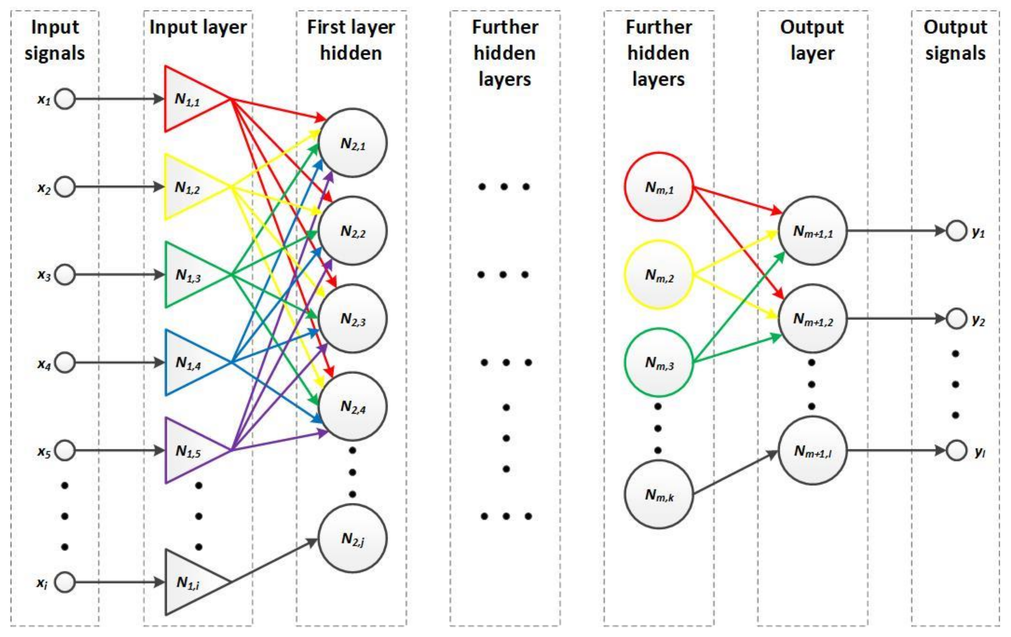
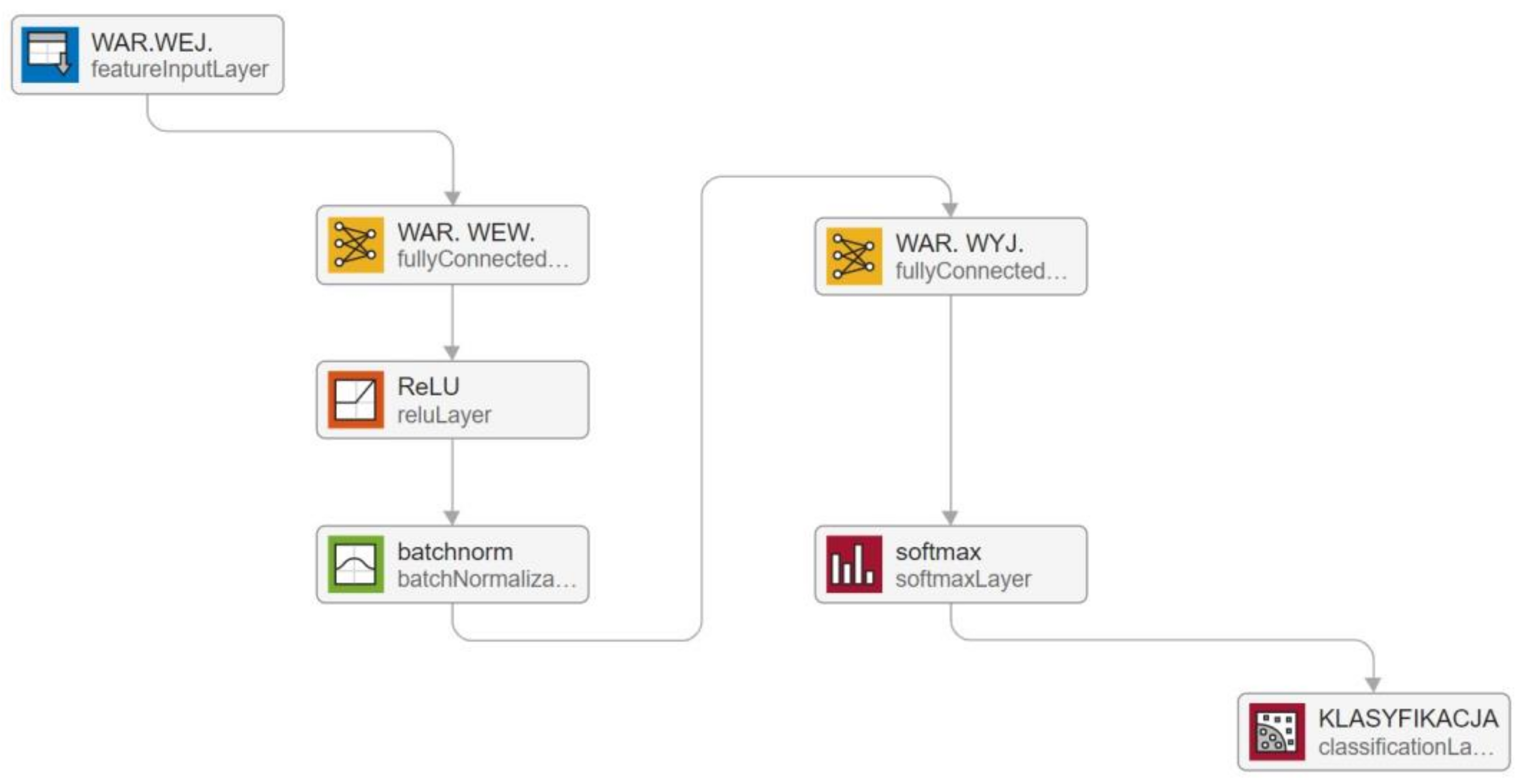
5. Structure of the Neural Network Used in the Classification System

A typical neural network used in classification problems consists of an input layer, one or more hidden layers, and an output layer (Figure 6). The number of neurons in the input and output layers depends on the number of input variables (selected from a ranking of signal features) and the number of states to be classified. The number of hidden layers and the number of neurons contained therein determine the network’s ability to obtain a correct classification result and are is usually selected experimentally or by means of appropriate algorithms [38,39].

The designed classification system using deep machine learning involved a network consisting of three layers, i.e., an input layer, an output layer, and a hidden layer with N, M, and Q nodes (neurons). A block diagram of the neural network (modeled in the MATLAB suite [40]), with additional blocks to normalize the data flow between the neurons of each layer, is provided in Figure 7.

The input layer (WAR. WEJ.) allowed the entry of data into the network and performed data normalization. This layer was composed of N input neurons, to which the values of the previously selected N most relevant (determined from the ranking) signal features were given. The entered values of the most relevant features were subjected to normalization, which involved obtaining data with a mean value of zero and a standard unit of standard deviation. The normalized feature input vector was written as follows:

$$x={\left(x_{1 },x_2 ,x_{3 },x_4 ,\dots x_N\right)}^T$$

(5)

Thus prepared, the data were further analyzed in the hidden layer (WAR. WEW.) composed of M nodes. The normalized input data were multiplied by a weight matrix (w_{i, j}) with the dimensions N × M, and a load vector (bj) with the dimensions M × 1 was added. This operation in mathematical notation was expressed as follows:

$$y_j={\displaystyle \sum }_{i=1}^N{x}_i·w_{i,j}+b_j$$

(6)

In order to speed up network training, input data are divided into blocks. The size of each data block affects the network’s learning time and classification accuracy and is usually chosen experimentally. In the work presented here, it was assumed that the 308 data points needed for network learning (representing 70% of the 441 available input data) would be divided into seven blocks containing 44 data points each. The batchnorm block first normalized the activation of each neuron by subtracting the mean value from the mini-batch (data block) and dividing it by the standard deviation of the mini-batch. The layer then shifted the input data by offset β, which was a variable in the learning process, and performed scaling by a scale factor (ϑ), which was also a variable in the learning process. Mathematically, the operation was calculated as follows:

$$\widehat{x_i}=\frac{x_i-{\mu }_b}{\sqrt{{\delta }_b^2-\epsilon }}$$

(7)

$$y_i=\vartheta ·\widehat{x_i}+\beta$$

(8)

where:

$\widehat{x_i}$—normalized i-th input;

${\mu }_b$—mean value of the data block;

${\delta }_b$—standard deviation from a data block;

ε—calculation constant (usually 1 × 10⁻⁶).

The nonlinear function ReLU was used as the function activating each node (neuron) of the network [24,41], which can be written as follows:

$$y_i=max\left[y_i,0\right]$$

(9)

The data prepared in this way were further analyzed in the output layer (WAR.WYJ.), which consisted of K neurons. The input data of this layer were multiplied by a weight matrix (w_i,q) with the dimensions M × K. Then, a load vector (bq) with the dimensions K × 1 was added. The next step involved activation by means of the activation function (φ), which was usually the Softmax function in classification issues.

The mathematical activation of an example neuron at the output (q) of the network is shown below:

$$z_q=\phi ·{\displaystyle \sum }_{q=1}^k\left({\displaystyle \sum }_{l=1}^M{y}_i·w_{i,q}+b_q\right)$$

(10)

The Softmax (φ) activation function calculated the probability P(z_q) that a variable given to the input of the network belonged to a given class (label) at the output of the network:

$$P\left(z_q\right)=\frac{exp\left(z_q\right)}{{\sum }_{q=1}^k\exp \left(z_q\right)}$$

(11)

The classification layer took the calculated value from the Softmax activation function and assigned the input variable to one of k mutually exclusive classes using the CE cross entropy function:

$$CE=-{\displaystyle \sum }_{i=1}^N{\displaystyle \sum }_{q=1}^k{t}_{i,q}·\ln z_{i,q}$$

(12)

where:

N—number of samples;

k—number of class-independent output variables;

t_i,q—belonging index of the i-th sample to the q-th class;

z_i,q—output value assigning the i-th sample (input) to the q-th class (output); probability and association by the network of the i-th input with the q-th output (class).

The normalized input vector of the designed system contained the five most relevant features (selected from each of the rankings), and the three operating states of the pump were classified:

• Pump in working order;
• Pump at its end of life;
• Worn-out pump.

The network structure consisted of:

• 5 neurons in the input layer;
• 3 neurons in the classification layer;
• 12 neurons in the hidden layer.

The number of neurons in the hidden layer was identified according to the following relationship [38]:

$$M=2·E+i$$

(13)

where:

M—number of neurons in the hidden (inner) layer;

E—number of neurons in the input layer;

i—constant from the interval: 0 ÷ 8 (i = 2 was assumed in the study).

The parameters of the designed network, including the number of activated variables and the variables to be learned, are summarized in

Table 4. Main network parameters.

Network Parameters
No.	Name	Type	Number of Activated Variables	Variables Subject to Learning
1	WAR. WEJ.	Input layer	5	-
2	WAR. WEW.	Inner layer	12	12 × 5 (weights), 12 × 1 (load)
3	ReLU	Activation	12	-
4	Batchnorm	Data normalization	12	12 × 1 (offset), 12 × 1 (scaling)
5	WAR. WYJ.	Output layer	3	3 × 12 (weights), 3 × 1 (load)
6	Softmax	Smoothing	3	-
7	KLASYFIKACJA	Classification	-	-

.

Network Training—Learning Parameters

After adopting the structure and parameters of the neural network, the next step was to subject it to training. In the training process, the stochastic gradient method [42] using the Adam (Adaptive moment estimation) solver was used to change the network parameters (weights and load). The network was trained using seven blocks of data (each block contained 44 data points for training (MiniBatchSize)). The maximum number of network training epochs was assumed to be equal to 500.

In addition, the training data were reshuffled before each training epoch, and the validation data (which accounted for 15% of the 441 available data points) were reshuffled before each network validation.

A summary of the parameters used in the network training and validation process is included in

Table 5. Parameters used in network training and validation process.

No.	Parameter Name	Parameter Value
1	Gradient Decay Factor	0.95
2	Squared Gradient Decay Factor	0.99
3	Epsilon	1 × 10−8
4	Initial Learn Rate	1 × 10−3
5	Learn Rate Schedule	‘none’
6	Learn Rate Drop Factor	0.1
7	Learn Rate Drop Period	10
8	L2Regularization	1 × 10−3
9	Gradient Threshold Method	‘l2norm’
10	Gradient Threshold	Inf.
11	Max Epochs	500
12	MiniBatch Size	44
13	Verbose	1
14	Verbose Frequency	50
15	Validation Data	66 × 6 table
16	Validation Frequency	20
17	Validation Patience	Inf.
18	Shuffle	every epoch
20	Execution Environment	gpu

.

Using the features of vibration signals and pressure signals determined earlier from the rankings, they were given to the network’s inputs for training and subsequent validation. The progress of network training in the learning and validation process is separately shown in the waveforms of changes in accuracy and network error for features obtained from vibration signals (Figure 8) and features obtained from pressure signals (Figure 9).

A quantitative measure of the accuracy of the waveforms and network errors was the RMS values determined from the waveforms during the learning and validation process. The RMS values were determined from the last three hundred epochs of the received waveforms (i.e., between 200 and 500 epochs) according to the following relationship:

$$x_{RMS}=\sqrt{\frac{1}{N}{\displaystyle \sum }_{n=1}^N{\left|x_i\right|}^2}$$

(14)

where:

$x_i$—value of the data string;

N—number of data points.

A summary of the calculated RMS values is shown in

Table 6. Accuracy and error values during training and network validation.

Diagnostic Signal Type	Method of Determining Features	Accuracy		Error
		Training (%)	Validation (%)	Training (-)	Validation (-)
Vibrations	MRMR	94	93.9	0.17	0.16
Static and dynamic pressure	MRMR	98.7	96.7	0.07	0.11

.

An accuracy evaluation of the learned models for classifying the wear state of the studied displacement pump was carried out in the testing process using the remaining 15% of the data (15% of the 441 available data) that had not been used before (in training and validating the models). The accuracy (acc) of pump condition classification by the developed models was calculated from the following relationship:

$$\mathrm{acc}=\frac{{\sum }_{\mathrm{l}}^{\mathrm{N}}\left(\widehat{y_{\mathrm{i}}}==y_l\right)}{N}·100\%$$

(15)

where:

$\widehat{y_i}$—estimated state of the pump at the i-th data point;

$y_l$—the actual state of the pump at the i-th data point;

N—the total number of data.

The error matrices of the networks’ classification of pump status, along with the calculated values of the accuracy coefficients, are shown below (Figure 10 and Figure 11) and in

Table 7. Accuracy of pump status classification.

Type of Diagnostic Signal	Method of Determining Features	Accuracy of acc Classifier (%)
Vibrations	MRMR	95.5
Static and dynamic pressure	MRMR	100

.

6. Analysis of Obtained Results and Final Conclusions

Following the analysis of the obtained test results of the learned diagnostic models, it should be noted that one hundred percent accuracy in classifying the wear state of the pump was achieved with a network trained on features obtained from pressure signals (both static and dynamic) and ranked using the MRMR algorithm. Another classifier tested using features obtained from vibrations measured at characteristic locations on the pump body achieved a classification accuracy of 95.5%, misclassifying three states of pump efficiency as the end of pump operation. The adopted structure of a three-layer neural classifier with additional blocks normalizing the data flow between neurons in each layer proved to be sufficient to conduct the classification of the wear state of the studied pump. The use of the minimum redundancy maximum relevance (MRMR) algorithm as a feature relevance ranking method for the designed deep machine learning system allowed the development of a classifier with relatively good classification accuracy, regardless of whether vibration signals measured at characteristic pump body sites or pressure signals recorded at the pump’s discharge port were used as input data. It should be emphasized that the obtained features were derived from signals measured across the entire range of pump operation, i.e., under stationary operating conditions (in a thermally steady state) and under non-stationary operating conditions (i.e., with a changing viscosity of the hydraulic fluid caused by the conversion of system power losses into heat).

In conclusion, it should be mentioned that using a deep machine learning system consisting of a three-layer neural network trained on the features of the measured signals ranked using the MRMR algorithm allowed the evaluation of the wear state of the analyzed displacement pump, providing a high degree of accuracy.

References

1. Merritt, H.E. Hydraulic Control Systems; John Wiley & Sons: New York, NY, USA, 1967. [Google Scholar]
2. Manring, N.D.; Fales, R.C. Hydraulic Control Systems, 2nd ed.; John Wiley & Sons: New York, NY, USA, 2019. [Google Scholar]
3. Manring, N. Fluid Power Pumps and Motors: Analysis, Design and Control; McGraw Hill Professional: New York, NY, USA, 2013. [Google Scholar]
4. Watton, J. Modelling, Monitoring and Diagnostic Techniques for Fluid Power Systems; Springer: Berlin, Germany, 2007. [Google Scholar]
5. Konieczny, J.; Stojek, J. Use of the K-Nearest Neighbour Classifier in Wear Condition Clssification of a Positive Displacement Pump. Sensors 2021, 21, 6247. [Google Scholar] [CrossRef]
6. Bensaad, D.; Soualhi, A.; Guillet, F. A new leaky piston identification method in an axial piston pump based on the extended Kalman filter. Measurement 2019, 148, 106921. [Google Scholar] [CrossRef]
7. Dabrowska, R.; Stetter, H.; Sasmito, H.; Kleinmann, S. Extended Kalman filter algorithm for advanced diagnosis of positive displacement pumps. In Proceedings of the 8th IFAC Symposium on Fault Detection, Supervision and Safety of Technical Processes (SAFEPROCESS), Mexico City, Mexico, 29–31 August 2012. [Google Scholar]
8. Grewal, M.S.; Andrews, A.P. Kalman Filtering Theory and Practice Using MATLAB; John Wiley & Sons: New York, NY, USA, 2008. [Google Scholar]
9. Asl, R.M.; Hagh, Y.S.; Simani, S.; Handroos, H. Adaptive square-root unscented Kalman filter: An experimental study of hydraulic actuator state estimation. Mech. Syst. Signal Process. 2019, 132, 670–691. [Google Scholar]
10. Bahrami, M.; Naraghi, M.; Zareinejad, M. Adaptive super-twisting observer for fault reconstruction in electro-hydraulic systems. ISA Trans. 2018, 76, 235–245. [Google Scholar] [CrossRef] [PubMed] [Green Version]
11. Stojek, J. Application of time-frequency analysis for diagnostics of valve plate wear in axial-piston pump. Arch. Mech. Eng. 2010, 57, 309–322. [Google Scholar] [CrossRef]
12. Goharrizi, A.Y.; Sepehri, N.A. Wavelet-Based Approach for External Leakage Detection and Isolation from Internal Leakage in Valve-Controlled Hydraulic Actuators. IEEE Trans. Ind. Electron. 2011, 58, 4374–4384. [Google Scholar] [CrossRef]
13. Goharrizi, A.Y.; Sepehri, N. Internal Leakage Detection in Hydraulic Actuators Using Empirical Mode Decomposition and Hilbert Spectrum. IEEE Trans. Instrum. Meas. 2012, 61, 368–378. [Google Scholar] [CrossRef]
14. Jiang, W.; Zheng, Z.; Zhu, Y.; Li, Y. Demodulation for hydraulic pump fault signals based on local mean decomposition and improved adaptive multiscale morphology analysis. Mech. Syst. Signal Process. 2015, 58–59, 179–205. [Google Scholar] [CrossRef]
15. Yang, J.; Xie, G.; Yang, Y.; Zhang, Y.; Liu, W. Deep model integrated with data correlation analysis for multiple intermittent faults diagnosis. ISA Trans. 2019, 95, 306–319. [Google Scholar] [CrossRef]
16. Hajnayeb, A.; Ghasemloonia, A.; Khadem, S.E.; Moradi, M.H. Application and comparison of an ANN-based feature selection method and the genetic algorithm in gearbox fault diagnosis. Exp. Syst. Appl. 2011, 38, 10205–10209. [Google Scholar] [CrossRef]
17. Pan, Z.Z.; Meng, Z.; Chen, Z.J.; Gao, W.Q.; Shi, Y. A two-stage method based on extreme learning machine for predicting the remaining useful life of rollingelement bearings. Mech. Syst. Signal. 2020, 144, 106899. [Google Scholar] [CrossRef]
18. Ji, X.; Ren, Y.; Tang, H.; Shi, C.; Xiang, J. An intelligent fault diagnosis approach based on Dempster-Shafer theory for hydraulic valves. Measurement 2020, 165, 108129. [Google Scholar] [CrossRef]
19. Zhao, R.; Yan, R.; Chen, Z.; Mao, K.; Wang, P.; Gao, R.X. Deep learning and its applications to machine health monitoring. Mech. Syst. Signal Process. 2019, 115, 213–237. [Google Scholar] [CrossRef]
20. Jegadeeshwaran, R.; Sugumaran, V. Fault diagnosis of automobile hydraulic brake system using statistical features and support vector machines. Mech. Syst. Signal Process. 2015, 52–53, 436–446. [Google Scholar] [CrossRef]
21. Lan, Y.; Hu, J.; Huang, J.; Niu, L.; Zeng, X.; Xiong, X.; Wu, B. Fault diagnosis on slipper abrasion of axial piston pump based on Extreme Learning Machine. Measurement 2018, 124, 378–385. [Google Scholar] [CrossRef]
22. Ji, X.; Ren, Y.; Tang, H.; Xiang, J. DSmT-based three-layer method using multi-classifier to detect faults in hydraulic systems. Mech. Syst. Signal Process. 2021, 153, 107513. [Google Scholar] [CrossRef]
23. Tiwari, R.; Bordoloi, D.J.; Dewangan, A. Blockage and cavitation detection in centrifugal pumps from dynamic pressure signal using deep learning algorithm. Measurement 2021, 173, 108676. [Google Scholar] [CrossRef]
24. Wang, S.; Xiang, J.; Zhong, Y. Hesheng Tang: A data indicator-based deep belief networks to detect multiple faults in axial piston pumps. Mech. Syst. Signal Process. 2018, 112, 154–170. [Google Scholar] [CrossRef]
25. Joshi, A.V. Machine Learning and Artificial Intelligence; Springer Nature: Cham, Switzerland, 2020. [Google Scholar]
26. Li, X.; Xu, Y.; Li, N.; Yang, B.; and Lei, Y. Remaining Useful Life Prediction With Partial Sensor Malfunctions Using Deep Adversarial Networks. IEEE/CAA J. Autom. Sin. 2023, 10, 121–134. [Google Scholar] [CrossRef]
27. Peng, H.C.; Long, F.; Ding, C. Feature Selection Based on Mutual Information: Criteria of Max-Dependency, Max-Relevance, and Min-Redundancy. IEEE Trans. Pattern Anal. Mach. Intell. 2005, 27, 1226–1238. [Google Scholar]
28. Guillon, M. Teoria i Obliczanie Układów Hydraulicznych; Wydawnictwo Naukowo Techniczne: Warszawa, Poland, 1966. [Google Scholar]
29. Ma, J.; Chen, J.; Li, J.; Li, Q.; Ren, C. Wear analysis of swash plate/slipper pair of axis piston hydraulic pump. Tribol. Int. 2015, 90, 467–472. [Google Scholar] [CrossRef]
30. Lyu, F.; Zhang, J.; Sun, G.; Xu, B.; Pan, M.; Huang, X.; Xu, H. Research on wear prediction of piston/cylinder pair in axial piston pumps. Wear 2020, 456–457, 203338. [Google Scholar] [CrossRef]
31. Roberts, M.J. Signals and Systems Analysis Using Transform Methods and MATLAB; McGraw-Hill Higher Education: New York, NY, USA, 2004. [Google Scholar]
32. Esfandiari, R.S. Numerical Methods for Engineers and Scientists Using MATLAB, 2nd ed.; CRC Press: Boca Raton, FL, USA; Taylor & Francis Group: Boca Raton, FL, USA, 2017. [Google Scholar]
33. Bin, G.F.; Gao, J.J.; Li, X.J.; Dhillon, B.S. Early fault diagnosis of rotating machinery based on wavelet packets—Empirical mode decomposition feature extraction and neural network. Mech. Syst. Signal Process. 2012, 27, 696–711. [Google Scholar] [CrossRef]
34. Kroese, D.P.; Botev, Z.I.; Taimre, T.; Vaisman, R. Data Science and Machine Learning: Mathematical and Statistical Methods; CRC Press: Boca Raton, FL, USA; Taylor & Francis Group: Boca Raton, FL, USA, 2017. [Google Scholar]
35. Bhattacharyya, S.; Bhaumik, H.; Mukherjee, A.; De, S. Machine Learning for a Big Data Analysis; Walter de Gruyter: Berlin, Germany, 2019. [Google Scholar]
36. Leis, J.W. Digital Signal Processing Using MATLAB for Students and Researchers; John Wiley & Sons: New York, NY, USA, 2011. [Google Scholar]
37. Darbellay, G.A.; Vajda, I. Estimation of the information by an adaptive partitioning of the observation space. IEEE Trans. Inf. Theory 1999, 45, 4. [Google Scholar] [CrossRef] [Green Version]
38. Samanta, B. Gear Fault Detection Using Artificial Neural Networks and Support Vector Machines with Genetic Algorithms. Mech. Syst. Signal Process. 2004, 18, 625–644. [Google Scholar] [CrossRef]
39. Meyes, R.; Lu, M.; de Puiseau, C.W.; Meisen, T. Ablation studies in artificial neural networks. arXiv 2019, arXiv:1901.08644. [Google Scholar]
40. Available online: https://www.mathworks.com/ (accessed on 1 September 2021).
41. Zhu, Y.; Li, G.; Wanga, R.; Tanga, S.; Su, H.; Cao, K. Intelligent fault diagnosis of hydraulic piston pump combining improved LeNet-5 and PSO hyperparameter optimization. Appl. Acoust. 2021, 183, 108336. [Google Scholar] [CrossRef]
42. Kingma, D.P.; Ba, J. Adam: A Method for Stochastic Optimization. In Proceedings of the 3rd International Conference for Learning Representations, San Diego, CA, USA, 7–9 May 2015. [Google Scholar]
Figure 1. Simplified design diagram of an axial piston pump with a swashplate: 1—shaft, 2—rotor, 3—piston, 4—sliding shoe, 5—swashplate, 6—valve plate, 7—bearing [28].
Energies 16 01408 g001
Figure 2. View of the vibration transducers mounted on the body of the tested pump.
Energies 16 01408 g002
Figure 3. Simplified diagram of the test bench: Pb—multi-piston pump being tested, Pw—booster pump, Zb—maximum valve, Zp—bypass valve, Zd—throttle valve, Zo—shut-off valve, Z1—non-return valve, Fs—low-pressure filter, Fw—filler filter, M—pressure gauge, n—rotometer, Q—flow meter, Ps—static pressure transducer, Pd—dynamic pressure transducer.
Energies 16 01408 g003
Figure 4. Significance ranking of features that satisfied the condition of the most significant applicability with minimal redundancy. Obtained from pump body vibration runs.
Energies 16 01408 g004
Figure 5. Significance ranking of the features that satisfied the condition of the greatest applicability with minimal redundancy. Obtained from the pressure waveforms (static and dynamic) in the discharge port of the pump.
Energies 16 01408 g005
Figure 6. General structure of a typical multilayer neural network.
Energies 16 01408 g006
Figure 7. Block structure of the network adopted for the classification of the wear state of the studied pump [40].
Energies 16 01408 g007
Figure 8. Waveforms of changes in accuracy and network error during training and validation process for the features of the received vibration signals.
Energies 16 01408 g008
Figure 9. Curves of changes in accuracy and network error during training and validation process for the features of the received pressure signals.
Energies 16 01408 g009
Figure 10. Matrix for classifying the wear state of the pump on the basis of features obtained from vibration signals.
Energies 16 01408 g010
Figure 11. Matrix for classifying the wear state of the pump based on features obtained from pressure signals.
Energies 16 01408 g011