Advanced Method of Variable Refrigerant Flow (VRF) Systems Designing to Forecast On-Site Operation—Part 1: General Approaches and Criteria

Abstract

All the energetic management and controlling strategies in ambient air conditioning systems (ACS) are aimed to match design load to current needs. This might be achieved by determining a rational value of design thermal load without overestimation that can minimize its deviation from the actual values. The application of variable refrigerant flow (VRF) systems with speed-regulated compressors (SRC) is considered as the most advanced trend in building air conditioning due to the ability of SRCs to cover changeable heat loads without lowering their efficiency. The level of load regulation by SRC is evaluated as the ratio of the load range, regulated by SCR, to the overall design load range. With this, the range of actual changeable loads is usually supposed to be covered by SRC entirely while keeping the rest, unregulated, and load range unchangeable. However, to confirm this, the rest load range behind the regulated one should be investigated to estimate the efficiency of SRC operation. Therefore, the approach to dividing the overall thermal load range of ambient air conditioning into the ranges of changeable and unchangeable loads to compare with those covered by SRC is used. From this approach, the method of rational designing and shearing a design refrigeration capacity in response to current loading, based on the principle of two-stage ambient air conditioning, has been widened on the VRF systems to estimate the efficiency of SCR application. This was realized by imposing the load ranges regulated by SRC onto the ranges of changeable and unchangeable loads within the overall range of actual loading. The proposed innovative criteria and indicators for rational shearing the load ranges to match current duties and load level evaluation can reveal the reserves for improving the efficiency of SRC compressor operation and the ACS of VRF type as a whole.

1. Introduction

Ambient air conditioning systems (ACS) are widely applied for comfortable air conditioning of buildings [1,2] as well as for combined energy supply to buildings and districts. ACS have achieved a wide application in trigeneration [3,4], integrated energy systems for combined cooling, heat and power (CCHP) [5,6], as well as in combustion engine cyclic air cooling, such as gas engines [7,8] and gas turbines [9,10], in transport applications [11,12]. Practically all ACS design and control methods are aimed for adaptation to actual climatic conditions [13,14]. The majority of methodological approaches [15,16] and heat recuperation solutions in energetic applications [17,18] can be efficiently introduced to building conditioning [19,20].

There is need for the application of efficient heat exchangers due to actual changeable thermal loads and to recuperate excessive energy. Many investigations are focused on intensifying heat transfer [21,22,23,24,25] and hydrodynamic enhancement [26,27], in particular, by mitigating flow maldistribution [28,29] and flow turbulization [30,31], evaporation [32,33] and condensation [34,35] in conditions of hydrodynamic instabilities [36,37] in conventional channels and minichannels [38,39], and their simulations [40,41]. Innovative circulation circuits [42,43], devices as ejectors [44,45] and aerothermopressors [46,47] are developed for efficient ACS applications in building and energetics.

The off-design modes dominate practically in the performance of all ACS [48,49]. One of the preferable reserves for enhancing energy efficiency of ACS consists in operating refrigeration compressors in nominal modes close to design thermal load and its rational distribution according to thermal load change in actual climatic conditions.

Generally, the overall range of current thermal loads of ACS involves the range of changeable thermal loads according to the parameters of incoming outdoor air and a relatively unchangeable share for further air conditioning with decreasing cooled air temperature from a definite threshold temperature to the set value [15,17,20].

It is preferable that a stable range of thermal load is offset when operating a conventional compressor in a mode close to the nominal value, while preconditioning of the outdoor air with significant fluctuations of thermal load requires regulation of refrigeration capacity by using a compressor with speed regulation (SRC). The load regulated level (LRL) of the SRC compressor must be consistent with the ranges with different behaviors of load change.

Numerous investigations are aimed to improve the operation efficiency of variable refrigerant flow (VRF) systems [50,51]. The VRF systems provide energy saving above 20% compared to variable air volume systems [52,53]. The VRF systems of combined type include outdoor and indoor subsystems [54,55]. The first subsystem is focused on treating the outdoor air to compensate for changeable thermal loads to avoid overloading the indoor subsystems [56,57].

However, despite the widespread application of SRC compressors, their load-regulated levels (LRL) rarely correspond to the required values and should be adopted to actual loading in site climatic conditions. Otherwise, the performance of the SRC compressor will be inefficient. There needs to be a development of ACS design methodology focused on matching the load regulation level of SRC compressors to climatic conditions.

There are many performance efficiency criteria [58,59] used as indicators [60,61] in thermal demand management (TDM) and primary energy-saving (PES) management methods [62,63] proposed for providing a high level of loading [64,65] and estimating the effect gained due to the application of combined energy systems [66,67], including ACS as a subsystem [68,69] or autonomic ACS of the VRF type with SRC compressors [70,71].

Despite the existence of various methods of multi-criteria analysis and synthesis [72,73], there is still a lack of studies on the methods for estimating the efficiency of SRC compressor applications in ACS of the VRF type from the point of providing full loading of the range, remaining outside the load regulation by SRC and usually supposed as full loaded one, which is not correct in real performance practice.

All the existing methods and criteria aimed at determining the design values of refrigeration capacity [74,75] are inappropriate for estimating the efficiency of SRC compressor performance with a definite load regulation level (LRL) and, consequently, for determining a required LRL of SRC compressors providing full loading in the unregulated range.

None of the above criteria [48,51,53,54,56,57,74] can assess actual loading of the range outside the load regulation, whereas the lack of load indicates a reduction in the performance efficiency of SRC.

All the energetic management and controlling strategies are aimed to match a design load to current needs through its reduction, which a priori testifies its overestimation and compressor and ACS oversizing as a result [4,60,61,62,63,64,65,74,75]. In reality, the SRC is an oversized compressor operating at part load but without lowering its efficiency. Moreover, the SRC runs in both ranges of thermal load simultaneously—regulated and unregulated refrigeration capacity. Therefore, it is preferable to develop a phenomenological basis for determining a rational value of design load of ACS to forecast its distribution with minimum deviation from the current duties and to adopt the load-regulated level (LRL) of SRC to this distribution at the design stage.

The corresponding criteria and indicators for rational shearing of the load to match the current duties and load level evaluation must reveal the reserves to improve the efficiency of the SRC compressor operation in ACS of the VRF type.

The aims of the research are to develop approaches, criteria and methods for variable refrigerant flow (VRF) systems designed through shearing the overall range of actual thermal loads on the ACS into ranges of changeable and unchangeable loads and, accordingly, to design refrigeration capacity that covers both ranges by a speed-regulated compressor SRC within its relevant ranges with and without regulations of refrigeration capacity to forecast its efficient on-site operation.

The following tasks are to be solved to reach these aims:

-

determine a rational design refrigeration capacity of an ambient air conditioning system (ACS) to provide practically maximum annual refrigeration energy generation according to its current consumption without overestimation;

-

develop a method for shearing the overall range of actual thermal loads on ACS into the ranges of changeable and unchangeable loads and, accordingly, adopt a design refrigeration capacity to cover both loads;

-

develop a method to determine the required load regulation level (LRL) of RSC proceeding from the relation between the ranges of changeable and unchangeable thermal loads as the objects for refrigeration capacity regulation by RSC and estimation of the RSC application efficiency by the level of loading both ranges, with emphasis on the second range.

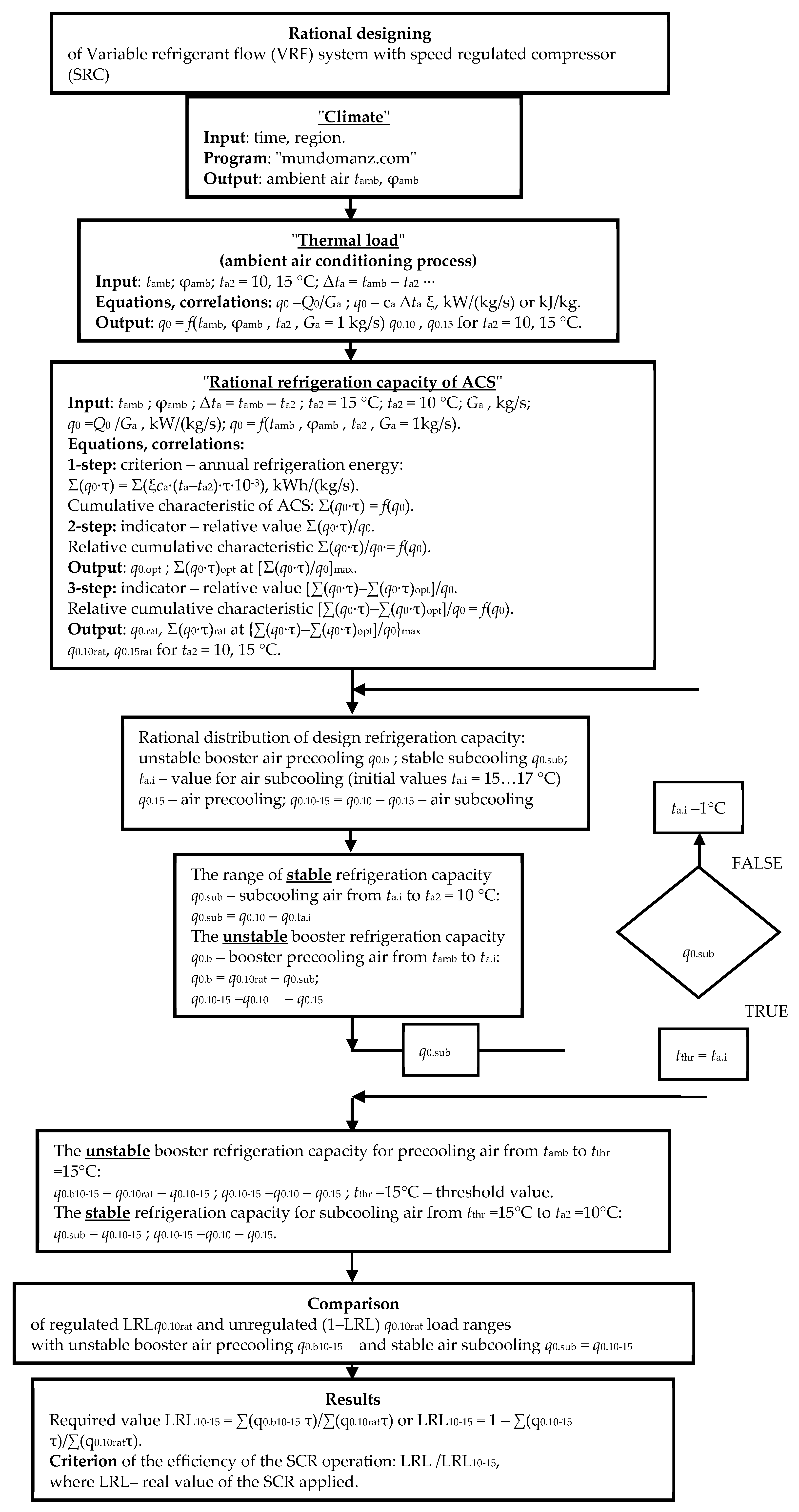
2. Methods

The following approaches and assumptions have been accepted in the design methodology of ACS to simplify quantifying the results of the analysis.

The ambient ACS as an autonomous system, the main subsystem of combined outdoor and indoor ACS of the VRF type [48,51,53,54,56,57,70,71], and the ranges of changeable and unchangeable thermal loads are accepted as the objects of investigation.

The efficiency of ACS performance is estimated by the efficiency of installed (design) refrigeration capacity utilization to cover current consumption without oversizing and depends on their thermal loading and time duration τ. Therefore, the annual refrigeration energy consumption Σ(Q₀∙τ) according to current needs Q₀∙τ is accepted as a primary criterion to define a design refrigeration capacity Q₀ of ACS.

For this, the annual refrigeration energy cumulative curve dependent on the refrigeration capacity Q₀ is received by summation of the current values:

Σ(Q₀∙τ) = f(Q₀).

(1)

To generalize the results and to extend them for any value of refrigeration capacity Q₀, the latter is used as the specific value q₀ = Q₀/G_a, which is related to air mass flow rate G_a:

q₀ = ξ∙c_a∙Δt_a, kW/(kg/s),

(2)

where Δt_a = (t_amb − t_a2);

t_amb—ambient air temperature, K or °C;

t_a2—set air temperature, accepted as the example in the investigation t_a2 = 10 °C;

ξ—relative heat ratio of latent and sensible heat to its sensible heat;

c_a—air specific heat, kJ/(kg·K).

The real input data on site of actual ambient air temperatures t_amb and relative humidity φ were taken by using the well-known and verified program “meteomanz” [76].

A specific annual refrigeration energy consumption:

Σ(q₀∙τ) = Σξ·c_a∙(t_a − t_a2)∙τ∙10⁻³, kWh/(kg/s).

(3)

Accordingly, the specific values of refrigeration capacity q_0.10 and refrigeration energy consumption q_0.10∙τ are required for conditioning the air to t_a2 = 10 °C.

The changes in the current actual specific refrigeration energy consumption q₀∙τ are considered by the rate of their annual summation ∑(q₀∙τ) increment that can build the annual refrigeration energy cumulative curve as a function of refrigeration capacity q₀: Σ(q₀∙τ) = f(q₀).

Thus, the rate of the annual refrigeration energy consumption ∑(q₀∙τ) increment according to refrigeration capacity q₀ as its relative value ∑(q₀∙τ)/q₀ is applied as an indicative criterion to determine the optimum value of specific refrigeration capacity q_0.opt, providing the maximum rate of annual specific refrigeration energy ∑(q₀∙τ) increment and minimum sizes of ACS accordingly (Figure 1a).

The rational value of designed specific refrigeration capacity q_0.rat, providing a close-to-maximum annual refrigeration energy production ∑(q₀∙τ) according to its current consumption, is associated with the second, local, maximum rate of the annual specific refrigeration energy production ∑(q₀∙τ) increment within its range beyond the first, global, maximum rate: q₀ > q_0opt and ∑(q₀∙τ) > ∑(q₀∙τ)_opt, accordingly (Figure 1b).

With this, a similar relative parameter [∑(q₀∙τ) − ∑(q₀∙τ)_opt]/q₀ is used as the indicator to choose a rational value q_0.rat, which can practically cover the maximum annual refrigeration energy consumption ∑(q₀∙τ) (Figure 1b). Such a method of rational design can reduce the designed specific refrigeration capacity q_0.rat by about 15 to 20% compared to its value q_0.max (Figure 1c) according to the widespread design practice based on the maximum value of current refrigeration consumption, which inevitably leads to chiller and ACS oversizing.

The rational value q_0.rat of the designed refrigeration capacity can offset the annual refrigeration consumption ∑(q₀∙τ)_rat = 48 MWh/(kg/s) close to its maximum value of 50 MWh/(kg/s) but at reduced designed refrigeration capacity q_0.10rat=35 kW/(kg/s) of less than q_0.10max = 42 kW/(kg/s) (Figure 1).

Further development of the methodology for rational design of ACS with regulated refrigeration capacity is aimed at developing a method for shearing the total designed refrigeration capacity according to current thermal loads into ranges with different behaviors regarding their change (Appendix A). The range of fluctuations of thermal load requires the application of a speed-regulated compressor (SRC), whereas the range of comparably unchangeable thermal load for deeper air conditioning to the final temperature, for example t_a2 = 10 °C, can be offset by a conventional compressor without refrigeration capacity regulation. In order to apply the compressor with refrigeration capacity regulation to offset both ranges of load, it is necessary to analyze the ratio between both ranges and to compare it to the level of refrigeration capacity regulation by the SRC, id est., the load-regulated level (LRL).

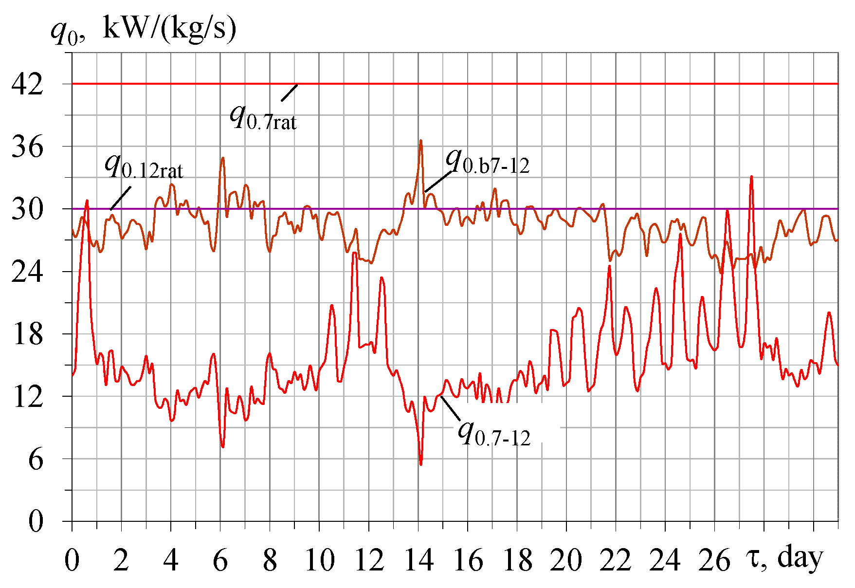
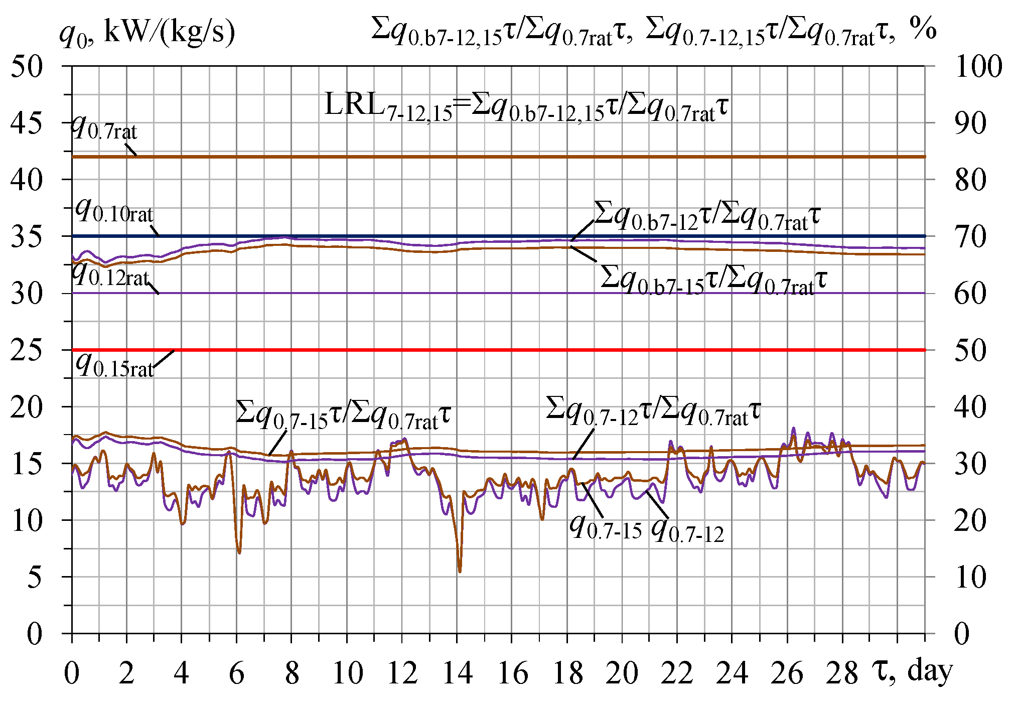
3. Results and Discussion

The total values of specific refrigeration capacities q_0.10, needed for conditioning outdoor air to 10 °C, have been sheared into the range of changeable values q_0.15 for preconditioning outdoor air to 15 °C and practically unchangeable refrigeration capacities q_0.10–15 for subsequent air conditioning from 15 to 10 °C. The calculation results for July 2017 in climatic conditions in southern Ukraine, Mykolayiv region, as an example of temperate climate, are presented in Figure 2.

As is seen from Figure 2a, when conditioning outdoor air to 10 °C, the thermal load fluctuations are great and follow their values for preconditioning outdoor air to 15 °C, which results in practically unchangeable refrigeration capacities q_0.10–15 for subsequent air conditioning from 15 to 10 °C. Issuing from the total designed rational value q_0.10rat and practically unchangeable part q_0.10–15 ≈ q_0.10rat − q_0.15rat (Figure 1), the remainder of the total value q_0.10rat as the booster one q_0.b10–15 = q_0.10rat − q_0.10–15 is available for preconditioning outdoor air to 15 °C.

Proceeding from stabilizing the loads when conditioning outdoor air below 15 °C, the latter is accepted as the threshold value t_thr = 15 °C to share the overall range of designed thermal load q_0.10rat (Figure 1) into extremely changeable load range q_0.15 when outdoor air preconditioning is t_a2 = 15 °C with a comparably unchangeable load range q_0.10–15 (Figure 2b). The range of unchangeable load q_0.10–15 is assumed as a basic part of the designed refrigeration capacity q_0.10rat, whereas the remainder of the total refrigeration capacity value q_0.10rat is supposed to be an available booster refrigeration capacity q_0.b10–15 intended for ambient air preconditioning to 15 °C and is defined as q_0.b15 = q_0.10rat − q_0.10–15 (Figure 2b).

The SRC with a load-regulated level of LRL = 0.5 is initially considered for simplifying the analyses.

The SRC is intended to cover the changeable load range evaluated as LRL·q_0.10rat according to its load-regulated level and to provide the stable operation of ACS within a range of load below (outside) the SRC regulated range, id est., within the range of less than (1–LRL) q_0.10rat = 0.5 q_0.10rat or q_0.10rat/2 = 0.5 q_0.10rat.

Therefore, it is quite reasonable to analyze the rest loads marked as q_0.10˂0.5 within the load range from the zero load to q_0.10rat/2 = 0.5 q_0.10rat, id est., without refrigeration capacity regulation, and to estimate the efficiency of SRC application by the level of loading (LL) of this range through comparing the loads q_0.10˂0.5 as partial loads to q_0.10rat/2 = 0.5, with q_0.10rat as the full one (Figure 3).

A lack of loading within the unregulated range q_0.10 ˂ q_0.10rat/2 is considered as exceeding q_{0.10rat/2ex˂0.5} = q_0.10rat/2 − q_0.10˂0.5 of the rational designed value of refrigeration capacity q_0.10rat/2 = q_0.10rat/2 over the actual loads marked as q_0.10˂0.5 (Figure 4).

The efficiency of the SCR compressor operation has to be analyzed taking into account the level of loading in the range from 0 to q_0.10rat/2, id est., the load range without refrigeration capacity regulation.

It can be estimated by the relative values q_0.10˂0.5/q_0.10rat/2 of the current refrigeration capacity q_0.10˂0.5 that refers to the corresponding part of the design refrigeration capacity q_0.10rat/2 (Figure 3) and by relative values ∑(q_0.10˂0.5 τ)/∑(q_0.10rat/2τ) of the monthly summarized refrigeration energy consumed within a load range without refrigeration capacity regulation ∑(q_0.10˂0.5 τ), referring to the refrigeration energy generated ∑(q_0.10rat/2τ) according to rational design values q_0.10rat/2 (Figure 5).

Corresponding values of current level of load LL_cur = q_0.10˂0.5/q_0.10rat/2 and monthly summarized LL = ∑(q_0.10˂0.5 τ)/∑(q_0.10rat/2τ) values are applied as indicative criteria. The value LL = 1.0 indicates the operation of SRC with maximum efficiency.

As Figure 6 shows, the level of loading LL for the unregulated range calculated as LL = ∑(q_0.10˂0.5 τ)/∑(q_0.10rat/2τ) is estimated by 80% to 88% of its full loading.

Thus, the level of loading LL for the unregulated range can indirectly indicate the efficiency of operating RSC with LRL = 0.5 as 80% to 88% values against a target value LL = 1.0.

The next step of analyses is aimed at determining the required value of LRL to provide the most efficient operation of RSC with the maximum level of loading for the range without refrigeration capacity regulation. This would be possible when the range of practically stable thermal load q_0.10–15 = q_0.10 − q_0.15 for further subsequent air conditioning to the final temperature of 10 °C rises to the rational designed value q_0.10rat/2 (Figure 7).

With this, the lack of thermal loads, characterized by the values of exceedance of rational refrigeration capacity q_0.10rat/2ex above the actual thermal loads q_0.10˂0.5 within a range without refrigeration capacity regulation (Figure 4), is reflected by corresponding increments of the rest booster thermal loads q_0.b10–15 (Figure 8), based on which the current LRL_10–15cur and summarized LRL_10–15 values are calculated.

This is also proven by the results of the calculated values LRL_10–15 and LRL_10–15cur proceeding from the relative values of current and summarized refrigeration energy consumed ∑(q_0.10˂0.5 τ)/∑(q_0.10rat/2τ), which can indirectly indicate the efficiency of operation of RSC with LRL = 0.5 issuing from the level of loading of the range without refrigeration capacity regulation below q_0.10rat/2.

Negligible fluctuations and practical coincidence of the values LRL_10–15 and LRL_10–15cur of about 0.71 testifies of the validity of the methodology developed and correct results of the calculation (Figure 8).

As Figure 8 shows, the needed value LRL_10–15 is ∑(q_0.b10–15 τ)/∑(q_0.10ratτ) = 0.72…0.75.

Thus, the required level of regulated load LRL_10–15 can be determined indirectly by using the comparatively stable load: LRL_10–15 = 1 − ∑(q_0.10–15 τ)/∑(q_0.10ratτ) as a trend line of the current values LRL_10–15cur = 1 − q_0.10–15/q_0.10rat (Figure 8).

The ratio ∑(q_0.10–15 τ)/∑(q_0.10ratτ) or q_0.10–15/q_0.10rat can be considered as an indicator for estimating the performance efficiency of SRC in ACS as well as for determining the required value of LRL in actual climatic conditions, and furthermore, for revealing the peculiarities of the threshold and target temperature influences on LRL.

This is proven by the results of the calculated summarized LRL_10–15 and current LRL_10–15cur values from the relative values of current basic thermal load values q_0.10–15/q_0.10rat for further air conditioning from 15 to 10 °C and of corresponding summarized refrigeration energy consumed ∑(q_0.10–15 τ)/∑(q_0.10ratτ), estimating the level of loading of the range without refrigeration capacity regulation below q_0.10rat/2, such that the basic thermal loads q_0.10–15 are involved in the range without refrigeration capacity regulation, id est., below q_0.10rat/2 (Figure 9).

As one can see, the values of ratio ∑(q_0.10–15 τ)/∑(q_0.10ratτ) = 0.25…0.28 (Figure 9) correspond to the required values of LRL_10–15 = ∑(q_0.b10–15 τ)/∑(q_0.10ratτ) equal to 0.72…0.75 (Figure 8) according to the correlation LRL_10–15 = 1 − ∑(q_0.10–15 τ)/∑(q_0.10ratτ) as settled above.

Thus, it is quite preferable to estimate the efficiency of the real SCR application by the ratio of its value of LRL = 0.5, for example, to the required values of LRL_10–15 = ∑(q_0.b10–15 τ)/∑(q_0.10ratτ) within 0.72…0.75. Therefore, the ratio LRL/LRL_10–15 can be applied as the criterion of the efficiency of the SCR application, in our example, LRL/LRL_10–15 ≈ 0.67…0.68, id est., about 67…68% compared to the required value LRL_10–15.

The validity of phenomenological simulation and analytically received correlations is proven by the results of calculations performed for increased threshold temperature t_a2 = 17 °C compared to t_a2 = 15 °C (Figure 10).

The higher threshold temperature t_thr, id est., the greater the range of comparably unchangeable load for subcooling the air from t_thr to the set value t_thr = 10 °C and closer to the range of the regulated refrigeration capacity q_0.10rat/2 (q_0.10–17 closer to q_0.10rat/2 compared to q_0.10–15), the more efficient the operation of the SRC compressors with 50% of LRL, due to more loading of the range of unregulated load (0…50%).

Conversely, the lower the threshold temperature t_thr (t_thr = 15 °C vs. 17 °C), the less effective the performance of the compressors with 50% of LRL, due to less loading of the unregulated load range (0…50%): q_0.10–15 < q_0.10rat/2, which requires a higher level of refrigeration capacity regulation (about 70% against 50%).

However, in temperate climates, the temperature 17 °C is higher than real t_thr = 15 °C, which is testified by greater fluctuations of q_0.10–17 against q_0.10–15 (Figure 10). Thus, the temperature 17 °C was assumed as the artificial threshold temperature just to investigate the peculiarities of its influence upon the efficiency of SCR performance from the point of loading of the unregulated range.

Meanwhile, at the same threshold temperature t_thr = 15 °C, the lower the target temperature, for instance t_a2 = 7 °C against t_a2 = 10 °C, the less the level of refrigeration capacity regulation that is required (Figure 11).

As can be seen, at the same threshold temperature t_thr = 15 °C and coinciding with the residual booster values q_0.b7–15 and q_0.b10–15, the relative booster refrigeration capacity values q_0.b7–15/q_0.7rat are less than q_0.b10–15/q_0.10rat because q_0.7rat is larger than q_0.10rat, id est., the SRC compressor with a lower level of regulated load, LRL = ∑(q_0.b7–15 τ)/∑(q_0.7ratτ), can be applied for deeper air conditioning to t_a2 = 7 °C as compared to LRL= ∑(q_0.10–15 τ)/∑(q_0.10ratτ), for air conditioning to t_a2 = 10 °C (Figure 12).

This is also approved by monthly values of booster-summarized refrigeration energy ∑(q_0.b7–12 τ) and ∑(q_0.b7–15ratτ) for air conditioning to the target temperature of 7 °C at the threshold temperatures 12 and 15 °C, accordingly (Figure 12).

As can be seen, at the same threshold temperature t_thr = 15 °C but for various set temperatures of t_a2 = 7 and 10 °C, the relative booster refrigeration capacity values q_0.b7–5/q_0.7rat are less than q_0.b10–15/q_0.10rat because q_0.7rat are larger than q_0.10rat. Therefore, the SRC compressor with the lower level of regulated load, LRL_7–15 = ∑(q_0.b7–15 τ)/∑(q_0.7ratτ), can be applied for deeper air conditioning to t_a2 = 7 °C as compared to LRL_10–15 =∑(q_0.10–15 τ)/∑(q_0.10ratτ), for air conditioning to t_a2 = 10 °C: LRL_7–15 = 0.67…0.68 against about LRL_10–15 = 0.75 (Figure 12).

The peculiarities of the influence of threshold temperatures on the level of regulated load LRL when conditioning outdoor air to the set temperature of 7 °C become clear from the calculated results in Figure 13 and Figure 14.

At the same set temperature t_a2 = 7 °C but at lowered threshold temperature t_thr = 12 °C, the SRC compressor with a higher level of regulated load, LRL= ∑(q_0.b7–12 τ)/∑(q_0.7ratτ) (Figure 14), should be applied as compared to LRL = ∑(q_0.b7–15 τ)/∑(q_0.7ratτ) for threshold temperature t_thr = 15 °C (Figure 12). This is due to the larger values of booster refrigeration capacities q_0.b7–12 according to the lower values of refrigeration capacities q_0.7–12 for subsequent air conditioning from 12 to 7 °C (Figure 13) as compared to the corresponding values of refrigeration capacities q_0.b7–15 and q_0.7–15 for air conditioning from 15 to 7 °C (Figure 11a).

As one can see, lowering the threshold temperature from 15 °C, for instance to t_a2 = 12 °C, at the same set temperature value 7 °C is accompanied by increasing the required level of regulated load LRL due to the widening booster regulated range of changeable loads from q_0.b7–15 (Figure 11a) to q_0.b7–12 (Figure 13), in its turn, due to narrowing the values of unregulated range for subcooling the air from t_a2 = 15 °C and t_a2 = 12 °C to t_a2 = 7 °C (Figure 11a and Figure 13). This practically coincides with the relatively stabilized values of ∑(q_0.7–12 τ)/∑(q_0.7ratτ) and ∑(q_0.7–15 τ)/∑(q_0.7ratτ) and LRL= ∑(q_0.b7–12 τ)/∑(q_0.7ratτ) and LRL = ∑(q_0.b7–15 τ)/∑(q_0.7ratτ), as the results testify that the choice of the temperature t_a2 = 15 °C as a threshold value is justified.

Thus, the expediency of a rational two-stage distribution of a designed refrigeration capacity, determined to practically cover the maximum annual refrigeration consumption that is reduced by 15 to 20% of the designed values compared to the conventional designing practice, and as the effective method for providing efficient operation of the SRC compressors and ACS of the VRF type entirely, was proven by the monthly summarized values of refrigeration energy consumption to cover the current duties through refrigerant capacity regulation by the SRC.

All the assumptions, correlations, criteria and indicative factors in the developed designing methodology have been approved by the phenomenological simulation of the ambient air cooling processes to determine their optimum parameters by using the basic heat balances (1–3), required minimal empirical data, and the real input data on current ambient air parameters (t_amb and φ_amb) through applying the well-known verified program “meteomanz”.

Furthermore, the proposed innovative approach to determine the rational value of refrigeration capacity based on the summarized refrigeration energy according to its actual consumption can avoid the inevitable errors caused by approximating the current thermal loads that are peculiar to conventional designing practice.

4. Conclusions

The changes in the current actual specific refrigeration energy consumption q₀∙τ are considered by the rate of their annual summation ∑(q₀∙τ) increment according to refrigeration capacity q₀, calculated as its relative value ∑(q₀∙τ)/q₀. The latter has been applied as an indicative criterion to determine the optimum value of specific refrigeration capacity q_0.opt, providing the maximum rate of annual specific refrigeration energy ∑(q₀∙τ) increment and the minimum sizes of ACS, accordingly.

The rational value of design specific refrigeration capacity q_0.rat, which can provide a close-to-maximum annual refrigeration energy production ∑(q₀∙τ) according to its current consumption, is determined as the second, local, maximum rate of the annual specific refrigeration energy production increment beyond the first, global, maximum rate.

The method for shearing the overall range of actual thermal loads on ACS into the ranges of changeable loads for ambient air precooling and the unchangeable load for further air subcooling to the target temperature t_a2, accordingly, was developed for adopting the designed refrigeration capacity to cover both of them.

The value of the threshold temperature t_thr to share the overall range of designed thermal load q_0.10rat into the ranges with different characters of loading is determined from stabilizing the loads below its magnitude.

For the first time in the design and operation practice for estimating the entire performance efficiency of speed-regulated compressors (SRC) and ACS of the VRF type, the unregulated range of refrigeration capacity was used as the object for analysis. Meanwhile, the opposite range of refrigeration capacity regulation was analyzed in existing practice for the RSC application efficiency estimation.

The advanced method to estimate the performance efficiency of SRC compressors through imposing the load ranges, regulated by SRC, on the ranges of changeable and unchangeable loads within the overall range of actual loading was developed. With this, the efficiency of SCR operation is estimated by the rate of loading of the unregulated range of the overall refrigeration capacity.

By varying the values of threshold t_thr and by setting t_t2 temperatures, the peculiarities of changing the load regulation level (LRL) of RSC and the correlation between unregulated range and the range of comparably stable load were revealed, and the favorable conditions for efficient application of SRC were investigated.

This method could determine the optimum (required) values of the load regulation level (LRL) of RSC compressors, providing full loading of the unregulated range of the overall refrigeration capacity and efficient implementation of RSC into any ACS of the VRF type for on-site climatic conditions.

The ratio of LRL of the real SCR to the required value of LRL providing full loading of the range outside the refrigeration capacity regulation is applied as a criterion for the efficiency of the SCR application.

References

1. Southard, L.E.; Liu, X.; Spitler, J.D. Performance of HVAC systems at ASHRAE HQ. ASHRAE J. 2014, 56, 14–24. [Google Scholar]
2. Gayeski, N.T.; Armstrong, P.R.; Norford, L.K. Predictive pre-cooling of thermo-active building systems with low-lift chillers. HVAC&R Res. 2012, 18, 858–873. [Google Scholar]
3. Radchenko, A.; Radchenko, M.; Mikielewicz, D.; Pavlenko, A.; Radchenko, R.; Forduy, S. Energy saving in trigeneration plant for food industries. Energies 2022, 15, 1163. [Google Scholar] [CrossRef]
4. Yang, Z.; Korobko, V.; Radchenko, M.; Radchenko, R. Improving thermoacoustic low temperature heat recovery systems. Sustainability 2022, 14, 12306. [Google Scholar] [CrossRef]
5. Maraver, D.; Sin, A.; Royo, J.; Sebastian, F. Assessment of CCHP systems based on biomass combustion for small-scale applications through a review of the technology and analysis of energy efficiency parameters. Appl. Energy 2013, 102, 1303–1313. [Google Scholar] [CrossRef]
6. Yang, Z.; Radchenko, R.; Radchenko, M.; Radchenko, A.; Kornienko, V. Cooling potential of ship engine intake air cooling and its realization on the route line. Sustainability 2022, 14, 15058. [Google Scholar] [CrossRef]
7. Shukla, A.K.; Sharma, A.; Sharma, M.; Mishra, S. Performance Improvement of Simple Gas Turbine Cycle with Vapor Compression Inlet Air Cooling. Mater. Today Proc. 2018, 5, 19172–19180. [Google Scholar] [CrossRef]
8. Kalhori, S.B.; Rabiei, H.; Mansoori, Z. Mashad trigeneration potential—An opportunity for CO2 abatement in Iran. Energy Conv. Manag. 2012, 60, 106–114. [Google Scholar] [CrossRef]
9. Radchenko, A.; Radchenko, N.; Tsoy, A.; Portnoi, B.; Kantor, S. Increasing the efficiency of gas turbine inlet air cooling in actual climatic conditions of Kazakhstan and Ukraine. AIP Conf. Proc. 2020, 2285, 030071. [Google Scholar] [CrossRef]
10. Shukla, A.K.; Singh, O. Impact of Inlet Fogging on the Performance of Steam Injected Cooled Gas Turbine Based Combined Cycle Power Plant. In Proceedings of the Gas Turbine India Conference, Bangalore, India, 7–8 December 2017. [Google Scholar]
11. Radchenko, M.; Mikielewicz, D.; Andreev, A.; Vanyeyev, S.; Savenkov, O. Efficient Ship Engine Cyclic Air Cooling by Turboexpander Chiller for Tropical Climatic Conditions. In Integrated Computer Technologies in Mechanical Engineering; ICTM 2020 Lecture Notes in Networks and Systems; Nechyporuk, M., Pavlikov, V., Kritskiy, D., Eds.; Springer: Cham, Switzerland, 2020; Volume 188, pp. 498–507. [Google Scholar]
12. Kornienko, V.; Radchenko, R.; Radchenko, M.; Radchenko, A.; Pavlenko, A.; Konovalov, D. Cooling cyclic air of marine engine with water-fuel emulsion combustion by exhaust heat recovery chiller. Energies 2022, 15, 248. [Google Scholar] [CrossRef]
13. Yu, Z.; Shevchenko, S.; Radchenko, M.; Shevchenko, O.; Radchenko, A. Methodology of Designing Sealing Systems for Highly Loaded Rotary Machines. Sustainability 2022, 14, 15828. [Google Scholar] [CrossRef]
14. Ravache, B.; Singh, R.; Dutton, S.M. Climate-Specific modeling and analysis for best-practice Indian office buildings 2015 Association. In Proceedings of the BS2015: 4th Conference of International Building Performance Simulation, Hyderabad, India, 7–9 December 2015; pp. 2190–2197. [Google Scholar]
15. Yang, Z.; Radchenko, M.; Radchenko, A.; Mikielewicz, D.; Radchenko, R. Gas turbine intake air hybrid cooling systems and a new approach to their rational designing. Energies 2022, 15, 1474. [Google Scholar] [CrossRef]
16. Radchenko, A.; Scurtu, I.-C.; Radchenko, M.; Forduy, S.; Zubarev, A. Monitoring the efficiency of cooling air at the inlet of gas engine in integrated energy system. Therm. Sci. 2022, 26, 185–194. [Google Scholar] [CrossRef]
17. Radchenko, A.; Radchenko, M.; Koshlak, H.; Radchenko, R.; Forduy, S. Enhancing the efficiency of integrated energy system by redistribution of heat based of monitoring data. Energies 2022, 15, 8774. [Google Scholar] [CrossRef]
18. Yang, Z.; Kornienko, V.; Radchenko, M.; Radchenko, A.; Radchenko, R. Research of Exhaust Gas Boiler Heat Exchange Surfaces with Reduced Corrosion when Water-fuel Emulsion Combustion. Sustainability 2022, 14, 11927. [Google Scholar] [CrossRef]
19. Radchenko, N.; Trushliakov, E.; Radchenko, A.; Tsoy, A.; Shchesiuk, O. Methods to determine a design cooling capacity of ambient air conditioning systems in climatic conditions of Ukraine and Kazakhstan. AIP Conf. Proc. 2020, 2285, 030074. [Google Scholar] [CrossRef]
20. Radchenko, M.; Radchenko, A.; Radchenko, R.; Kantor, S.; Konovalov, D.; Kornienko, V. Rational loads of turbine inlet air absorption-ejector cooling systems. Proc. Inst. Mech. Eng. Part A J. Power Energy 2021, 236, 095765092110454. [Google Scholar] [CrossRef]
21. Kruzel, M.; Bohdal, T.; Dutkowski, K.; Kuczyński, W.; Chliszcz, K. Current Research Trends in the Process of Condensation of Cooling Zeotropic Mixtures in Compact Condensers. Energies 2022, 15, 2241. [Google Scholar] [CrossRef]
22. Yang, Z.; Kornienko, V.; Radchenko, M.; Radchenko, A.; Radchenko, R.; Pavlenko, A. Capture of pollutants from exhaust gases by low-temperature heating surfaces. Energies 2022, 15, 120. [Google Scholar] [CrossRef]
23. Pavlenko, A.M.; Koshlak, H. Application of thermal and cavitation effects for heat and mass transfer process intensification in multicomponent liquid media. Energies 2021, 14, 7996. [Google Scholar] [CrossRef]
24. Pavlenko, A. Energy conversion in heat and mass transfer processes in boiling emulsions. Therm. Sci. Eng. Prog. 2020, 15, 00439. [Google Scholar] [CrossRef]
25. Pavlenko, A. Change of emulsion structure during heating and boiling. Int. J. Energy Clean Environ. 2019, 20, 291–302. [Google Scholar] [CrossRef]
26. Kruzel, M.; Bohdal, T.; Dutkowski, K.; Radchenko, M. The Effect of Microencapsulated PCM Slurry Coolant on the Efficiency of a Shell and Tube Heat Exchanger. Energies 2022, 15, 5142. [Google Scholar] [CrossRef]
27. Dąbrowski, P.; Klugmann, M.; Mikielewicz, D. Channel Blockage and Flow Maldistribution during Unsteady Flow in a Model Microchannel Plate Heat Exchanger. J. Appl. Fluid Mech. 2019, 12, 1023–1035. [Google Scholar] [CrossRef]
28. Dąbrowski, P.; Klugmann, M.; Mikielewicz, D. Selected studies of flow maldistribution in a minichannel plate heat exchanger. Arch. Thermodyn. 2017, 38, 135–148. [Google Scholar] [CrossRef] [Green Version]
29. Kumar, R.; Singh, G.; Mikielewicz, D. A New Approach for the Mitigating of Flow Maldistribution in Parallel Microchannel Heat Sink. J. Heat Transf. 2018, 140, 72401–72410. [Google Scholar] [CrossRef]
30. Kumar, R.; Singh, G.; Mikielewicz, D. Numerical Study on Mitigation of Flow Maldistribution in Parallel Microchannel Heat Sink: Channels Variable Width versus Variable Height Approach. J. Electron. Packag. 2019, 141, 21009–21011. [Google Scholar] [CrossRef]
31. Yaïci, W.; Ghorab, M.; Entchev, E. 3D CFD study of the effect of inlet air flow maldistribution on plate-fin-tube heat exchanger design and thermal–hydraulic performance. Int. J. Heat Mass Transf. 2016, 101, 527–541. [Google Scholar] [CrossRef]
32. Mikielewicz, D.; Klugmann, M.; Wajs, J. Flow boiling intensification in minichannels by means of mechanical flow turbulising inserts. Int. J. Therm. Sci. 2013, 65, 79–91. [Google Scholar] [CrossRef]
33. Bohdal, T.; Kuczynski, W. Boiling of R404A refrigeration medium under the conditions of periodically generated disturbances. Heat Transf. Eng. 2011, 32, 359–368. [Google Scholar] [CrossRef]
34. Dutkowski, K.; Kruzel, M. Microencapsulated PCM slurries’ dynamic viscosity experimental investigation and temperature ependent prediction model. Int. J. Heat Mass Transf. 2019, 145, 118741. [Google Scholar] [CrossRef]
35. Wajs, J.; Mikielewicz, D.; Jakubowska, B. Performance of the domestic micro ORC equipped with the shell-and-tube condenser with minichannels. Energy 2018, 157, 853–861. [Google Scholar] [CrossRef]
36. Kuczyński, W.; Kruzel, M.; Chliszcz, K. A Regressive Model for Periodic Dynamic Instabilities during Condensation of R1234yf and R1234ze Refrigerants. Energies 2022, 15, 2117. [Google Scholar] [CrossRef]
37. Kuczyński, W.; Kruzel, M.; Chliszcz, K. Regression Model of Dynamic Pulse Instabilities during Condensation of Zeotropic and Azeotropic Refrigerant Mixtures R404A, R448A and R507A in Minichannels. Energies 2022, 15, 1789. [Google Scholar] [CrossRef]
38. Liao, G.; Li, Z.; Zhang, F.; Liu, L.E.J. A Review on the Thermal-Hydraulic Performance and Optimization of Compact Heat Exchangers. Energies 2021, 14, 6056. [Google Scholar] [CrossRef]
39. Blecich, P. Experimental investigation of the effects of airflow nonuniformity on performance of a fin-and-tube heat exchanger. Int. J. Refrig. 2015, 59, 65–74. [Google Scholar] [CrossRef]
40. Korzen, A.; Taler, D. Modeling of transient response of a plate fin and tube heat exchanger. Int. J. Therm. Sci. 2015, 92, 188–198. [Google Scholar] [CrossRef]
41. Taler, D. Mathematical modeling and control of plate fin and tube heat exchangers. Energy Convers. Manag. 2015, 96, 452–462. [Google Scholar] [CrossRef]
42. Yu, Z.; Løvås, T.; Konovalov, D.; Trushliakov, E.; Radchenko, M.; Kobalava, H.; Radchenko, R.; Radchenko, A. Investigation of thermopressor with incomplete evaporation for gas turbine intercooling systems. Energies 2023, 16, 20. [Google Scholar] [CrossRef]
43. Kornienko, V.; Radchenko, R.; Konovalov, D.; Andreev, A.; Pyrysunko, M. Characteristics of the Rotary Cup Atomizer Used as Afterburning Installation in Exhaust Gas Boiler Flue. In Advances in Design, Simulation and Manufacturing III (DSMIE 2020); Ivanov, V., Pavlenko, I., Liaposhchenko, O., Machado, J., Edl, M., Eds.; Lecture Notes in Mechanical Engineering; Springer: Cham, Switzerland, 2020; pp. 302–311. [Google Scholar] [CrossRef]
44. Butrymowicz, D.; Gagan, J.; Śmierciew, K.; Łukaszuk, M.; Dudar, A.; Pawluczuk, A.; Łapiński, A.; Kuryłowic, A. Investigations of prototype ejection refrigeration system driven by low grade heat. HTRSE-2018 E3S Web Conf. 2020, 70, 03002. [Google Scholar] [CrossRef]
45. Radchenko, R.; Radchenko, N.; Tsoy, A.; Forduy, S.; Zybarev, A.; Kalinichenko, I. Utilizing the heat of gas module by an absorption lithium-bromide chiller with an ejector booster stage. AIP Conf. Proc. 2020, 2285, 030084. [Google Scholar] [CrossRef]
46. Yang, Z.; Konovalov, D.; Radchenko, M.; Radchenko, R.; Kobalava, H.; Radchenko, A.; Kornienko, V. Analyzing the efficiency of thermopressor application for combustion engine cyclic air cooling. Energies 2022, 15, 2250. [Google Scholar] [CrossRef]
47. Konovalov, D.; Radchenko, M.; Kobalava, H.; Radchenko, A.; Radchenko, R.; Kornienko, V.; Maksymov, V. Research of characteristics of the flow part of an aerothermopressor for gas turbine intercooling air. Proc. Inst. Mech. Eng. Part A J. Power Energy 2021, 236, 4. [Google Scholar] [CrossRef]
48. Im, P.; Malhotra, M.; Munk, J.D.; Lee, J. Cooling season full and part load performance evaluation of variable refrigerant flow (VRF) system using an occupancy simulated research building. In Proceedings of the 16th International Refrigeration and Air Conditioning Conference at Purdue, West Lafayette, IN, USA, 11–14 July 2016. [Google Scholar]
49. Canova, A.; Cavallero, C.; Freschi, F.; Giaccone, L.; Repetto, M.; Tartaglia, M. Optimal energy management. IEEE Ind. Appl. Mag. 2009, 15, 62–65. [Google Scholar] [CrossRef]
50. Radchenko, N.; Radchenko, A.; Tsoy, A.; Mikielewicz, D.; Kantor, S.; Tkachenko, V. Improving the efficiency of railway conditioners in actual climatic conditions of operation. AIP Conf. Proc. 2020, 2285, 030072. [Google Scholar] [CrossRef]
51. Liu, C.; Zhao, T.; Zhang, J. Operational electricity consumption analyze of VRF air conditioning system and air conditioning system based on building energy monitoring and management system. Procedia Eng. 2015, 121, 1856–1863. [Google Scholar] [CrossRef] [Green Version]
52. Khatri, R.; Joshi, A. Energy performance comparison of inverter based variable refrigerant flow unitary AC with constant volume unitary AC. Energy Procedia 2017, 109, 18–26. [Google Scholar] [CrossRef]
53. Park, D.Y.; Yun, G.; Kim, K.S. Experimental evaluation and simulation of a variable refrigerant-flow (VRF) air-conditioning system with outdoor air processing unit. Energy Build 2017, 146, 122–140. [Google Scholar] [CrossRef]
54. Thornton, B.; Wagner, A. Variable Refrigerant Flow Systems; Pacific Northwest National Laboratory: Seattle, WA, USA, 2012. Available online: http://www.gsa.gov/portal/mediaId/197399/fileName/GPG_Variable_Refrigerant_Flow_12-2012.action (accessed on 19 January 2020).
55. Chen, J.; Xie, W. Analysis on load-undertaking of fan coil unit with fresh air system. Adv. Mater. Res. 2013, 614, 678–681. [Google Scholar] [CrossRef]
56. Zhu, Y.; Jin, X.; Du, Z.; Fang, X.; Fan, B. Control and energy simulation of variable refrigerant flow air conditioning system combined with outdoor air processing unit. Appl. Therm. Eng. 2014, 64, 385–395. [Google Scholar] [CrossRef]
57. Lee, J.H.; Yoon, H.J.; Im, P.; Song, Y.H. Verification of energy reduction effect through control optimization of supply air temperature in VRF-OAP system. Energies 2018, 11, 49. [Google Scholar] [CrossRef]
58. Radchenko, M.; Radchenko, A.; Mikielewicz, D.; Radchenko, R.; Andreev, A. A novel degree-hour method for rational design loading. Proc. Inst. Mech. Eng. Part A J. Power Energy 2022. [Google Scholar] [CrossRef]
59. Suamir, I.N.; Tassou, S.A. Performance evaluation of integrated trigeneration and CO2 refrigeration systems. Appl. Therm. Eng. 2013, 50, 1487–1495. [Google Scholar] [CrossRef]
60. Ortiga, J.; Bruno, J.C.; Coronas, A. Operational optimization of a complex trigeneration system connected to a district heating and cooling network. Appl. Therm. Eng. 2013, 50, 1536–1542. [Google Scholar] [CrossRef]
61. Rodriguez-Aumente, P.A.; Rodriguez-Hidalgo, M.d.C.; Nogueira, J.I.; Lecuona, A.; Venegas, M.d.C. District heating and cooling for business buildings in Madrid. Appl. Therm. Eng. 2013, 50, 1496–1503. [Google Scholar] [CrossRef]
62. Freschi, F.; Giaccone, L.; Lazzeroni, P.; Repetto, M. Economic and environmental analysis of a trigeneration system for food-industry: A case study. Appl. Energy 2013, 107, 157–172. [Google Scholar] [CrossRef]
63. Radchenko, A.; Radchenko, M.; Trushliakov, E.; Kantor, S.; Tkachenko, V. Statistical Method to Define Rational Heat Loads on Railway Air Conditioning System for Changeable Climatic Conditions. In Proceedings of the 5th International Conference on Systems and Informatics, ICSAI 2018, Nanjing, Jiangsu, China, 10–12 November 2018; pp. 1294–1298. [Google Scholar] [CrossRef]
64. Cardona, E.; Piacentino, A. A methodology for sizing a trigeneration plant in mediterranean areas. Appl. Therm. Eng. 2003, 23, 15. [Google Scholar] [CrossRef]
65. Fumo, N.; Mago, P.J.; Smith, A.D. Analysis of combined cooling, heating, and power systems operating following the electric load and following the thermal load strategies with no electricity export. Proc. Inst. Mech. Eng. Part A J. Power Energy 2011, 225, 1016–1025. [Google Scholar] [CrossRef]
66. Giaccone, L.; Canova, A. Economical comparison of CHP systems for industrial user with large steam demand. Appl. Energy 2009, 86, 904–914. [Google Scholar] [CrossRef] [Green Version]
67. Kavvadias, K.C.; Tosios, A.P.; Maroulis, Z.B. Design of a combined heating, cooling and power system: Sizing, operation strategy selection and parametric analysis. Energy Convers. Manag. 2010, 51, 833–845. [Google Scholar] [CrossRef]
68. Konovalov, D.; Trushliakov, E.; Radchenko, M.; Kobalava, G.; Maksymov, V. Research of the aerothermopresor cooling system of charge air of a marine internal combustion engine under variable climatic conditions of operation. In Advanced Manufacturing Processes: Selected Papers from the Grabchenko’s International Conference on Advanced Manufacturing Processes (InterPartner-2019), September 10–13, 2019, Odessa, Ukraine; Tonkonogyi, V., Ivanov, V., Trojanowska, J., Oborskyi, G., Edl, M., Kuric, I., Pavlenko, I., Dasic, P., Eds.; Lecture Notes in Mechanical Engineering; Springer: Cham, Switzerland, 2020; pp. 520–529. [Google Scholar] [CrossRef]
69. Popli, S.; Rodgers, P.; Eveloy, V. Trigeneration scheme for energy efficiency enhancement in a natural gas processing plant through turbine exhaust gas waste heat utilization. Appl. Energy 2012, 93, 623–636. [Google Scholar] [CrossRef]
70. Lee, Y.; Kim, W. Development of an Optimal Start Control Strategy for a Variable Refrigerant Flow (VRF) System. Energies 2021, 14, 271. [Google Scholar] [CrossRef]
71. Chua, K.J.; Chou, S.K.; Yang, W.M.; Yan, J. Achieving better energy-efficient air conditioning—A review of technologies and strategies. Appl. Energy 2013, 104, 87–104. [Google Scholar] [CrossRef]
72. Carvalho, M.; Lozano, M.A.; Serra, L.M. Multicriteria synthesis of trigeneration systems considering economic and environmental aspects. Appl. Energy 2012, 91, 245–254. [Google Scholar] [CrossRef]
73. Geldermann, J.; Rentz, O. Multi-criteria analysis for the assessment of environmentally relevant installations. J. Ind. Ecol. 2020, 9, 127–142. [Google Scholar] [CrossRef]
74. Piacentino, A.; Cardona, F. EABOT—Energetic Analysis as a Basis for robust Optimization of Trigeneration systems by linear programming. Energy Convers. Manag. 2008, 49, 3006–3016. [Google Scholar] [CrossRef]
75. Forsyth, J.L. Gas turbine inlet air chilling for LNG. IGT Int. Liq. Nat. Gas Conf. Proc. 2013, 3, 1763–1778. [Google Scholar]
76. Available online: http://www.meteomanz.com (accessed on 1 January 2020).
Figure 1. Specific annual refrigeration energy consumption ∑(q0 ∙τ), optimum q0.opt and rational q0.rat values of specific refrigeration capacities while cooling ambient air to 10 and 15 °C in southern Ukraine (temperate climate), 2017: (a) determining of q0.opt; (b) determining of q0.rat; (c) generalized graphs for q0.opt and q0.rat; Δq0.10 = q0.10maxq0.10rat and Δq0.15 = q0.15maxq0.15rat.
Energies 16 01381 g001
Figure 2. The current values of specific refrigeration capacities q0.15 and q0.10 required for outdoor air conditioning to 15 and 10 °C, refrigeration capacities q0.10–15 for subsequent air conditioning from 15 to 10 °C, (a) as well as available booster values q0.b10–15 as the rest, remaining for outdoor air conditioning to 15 °C (b): q0.10–15 = q0.10q0.15; q0.b10–15 = q0.10q0.10–15.
Energies 16 01381 g002
Figure 3. Actual values of specific refrigeration capacities q0.10 required for outdoor air conditioning to 10 °C, a part load q0.10>0.5 of q0.10 within a range of refrigeration capacity regulated from q0.10rat/2 to q0.10rat and the rest part q0.10˂0.5 within the unregulated range from 0 to q0.10rat/2: q0.10rat/2 = 0.5, q0.10rat; q0.10 = q0.10>0.5 + q0.10˂0.5, where q0.10>0.5 is marked for q0.10 > 0.5 q0.10rat, and q0.10˂0.5 for q0.10 < 0.5 q0.10rat.
Energies 16 01381 g003
Figure 4. Actual values of thermal load q0.10 when cooling the air to 10 °C; the rest parts q0.10˂0.5 of q0.10 within the unregulated range from 0 to q0.10rat/2; values of rational refrigeration capacity q0.10rat/2 exceed q0.10rat/2ex above the actual thermal loads q0.10˂0.5 within the unregulated range from 0 to q0.10rat/2: q0.10rat/2ex˂0.5 = q0.10rat/2q0.10˂0.5; q0.10˂0.5 is marked for q0.10 < 0.5 q0.10rat.
Energies 16 01381 g004
Figure 5. Actual values of thermal load q0.10 when cooling the air to 10 °C; relative values q0.10˂0.5/q0.10rat/2 of current refrigeration capacity q0.10˂0.5 referring to q0.10rat/2; relative values of monthly summarized refrigeration energy consumed ∑(q0.10˂0.5 τ)/∑(q0.10rat/2τ) referring to refrigeration energy generated ∑(q0.10rat/2τ) according to the design value q0.10rat/2: LLcur = q0.10˂0.5 /q0.10rat/2; LL = ∑(q0.10˂0.5 τ)/∑(q0.10rat/2τ).
Energies 16 01381 g005
Figure 6. Actual values of thermal load q0.10 when cooling the air to 10 °C; the rest parts q0.10˂0.5 of q0.10 within the unregulated load range; summarized refrigeration energy consumed ∑(q0.10˂0.5 τ); generated ∑(q0.10rat/2τ) according to rational value q0.10rat/2 within the unregulated load range and relative values of summarized refrigeration energy consumed ∑(q0.10˂0.5 τ)/∑(q0.10rat/2τ): LL = ∑(q0.10˂0.5 τ)/∑(q0.10rat/2τ).
Energies 16 01381 g006
Figure 7. Actual values of refrigeration capacities q0.10 required for conditioning outdoor air to 10 °C; the values q0.10–15 for further air conditioning from 15 to 10 °C; residual booster values q0.b10–15: q0.b10–15 = q0.10ratq0.10–15; q0.10–15 = q0.10q0.15.
Energies 16 01381 g007
Figure 8. Actual values of refrigeration capacities q0.10–15 for further air conditioning from 15 to 10 °C and residual booster values q0.b10–15, relative booster thermal load values q0.b10–15/q0.10rat and corresponding relative summarized booster refrigeration energy ∑(q0.b10–15 τ)/∑(q0.10ratτ): LRL10–15 = ∑(q0.b10–15 τ)/∑(q0.10ratτ); LRL10–15cur = q0.b10–15/q0.10rat; q0.b10–15 = q0.10ratq0.10–15; q0.10–15 = q0.10q0.15; q0.10rat/2ex˂0.5 = q0.10rat/2q0.10˂0.5; q0.10˂0.5 is marked for q0.10 < 0.5 q0.10rat.
Energies 16 01381 g008
Figure 9. Actual values of refrigeration capacities q0.10–15 for further air conditioning from 15 to 10 °C and residual booster values q0.b10–15; relative basic thermal load values q0.10–15/q0.10rat for further air conditioning from 15 to 10 °C; corresponding averaged summarized refrigeration energy consumed ∑(q0.10–15 τ)/∑(q0.10ratτ): q0.b15 = q0.10ratq0.10–15; q0.10–15 = q0.10q0.15.
Energies 16 01381 g009
Figure 10. Actual values of refrigeration capacities q0.10–15,17 for subcooling the air from 15 and 17 °C to 10 °C; corresponding relative summarized refrigeration energy consumed for subcooling the air from 15 and 17 °C to 10 °C ∑(q0.10–15,17 τ)/∑(q0.10ratτ); relative summarized residual booster refrigeration energy available for precooling the ambient air to 15 and 17 °C: ∑(q0.b10–15,17 τ)/∑(q0.10ratτ): q0.10–15,17 = q0.10q0.15,17; q0.b10–15,17 = q0.10ratq0.10–15,17.
Energies 16 01381 g010
Figure 11. Actual values of refrigeration capacities q0.7–15 for air conditioning from 15 to 7 °C and residual booster values q0.b7–15; relative booster refrigeration capacities values q0.b7–15 /q0.7rat (a); corresponding refrigeration capacities q0.10–15 and q0.b10–15 and relative booster refrigeration capacities values q0.b10–15/q0.10rat (b) for air conditioning to the set temperatures of 7 and 10 °C, accordingly: q0.b7,10–15 = q0.7,10ratq0.15; q0.7,10–15 = q0.7,10q0.15 for air conditioning to 7 and 10 °C.
Energies 16 01381 g011
Figure 12. Actual values of refrigeration capacities q0.10–15 and q0.7–15 for subcooling air from the threshold values of 15 to 10 and 7 °C and corresponding relative summarized refrigeration energy consumed in unregulated ranges for subcooling the air ∑(q0.10–15 τ)/∑(q0.10ratτ) and ∑(q0.7–15 τ)/∑(q0.7ratτ), corresponding to relative summarized refrigeration energy consumed in booster regulated ranges for precooling the air ∑(q0.b10–15 τ)/∑(q0.10ratτ) and ∑(q0.b7–15 τ)/∑(q0.7ratτ) to the threshold value of 15 °C: q0.10,7–15 = q0.10,7q0.15 for subcooling air from 15 to 10 and 7 °C.
Energies 16 01381 g012
Figure 13. Actual values of refrigeration capacities q0.7–12 for air conditioning from 12 to 7 °C and residual booster values q0.b7–12; relative booster refrigeration capacities values q0.b7–12/q0.7rat for air conditioning to target temperature 7 °C at the threshold temperature 12 °C: q0.b7–12 = q0.7ratq0.12; q0.7–12 = q0.7q0.12.
Energies 16 01381 g013
Figure 14. Actual values of refrigeration capacities q0.7–12 and q0.7–15 for subcooling the air from 12 and 15 to 7 °C, corresponding to relative values of averaged summarized refrigeration energy consumed in unregulated ranges ∑(q0.7–12 τ)/∑(q0.7ratτ) and ∑(q0.7–15 τ)/∑(q0.7ratτ) and in regulated ranges as LRL = ∑(q0.b7–12 τ)/∑(q0.7ratτ) and LRL = ∑(q0.b7–15 τ)/∑(q0.7ratτ) for precooling the ambient air to the temperatures 12 and 15 °C as threshold values: q0.b7–12/15 = q0.7ratq0.12/15; q0.7–12/15 = q0.7q0.12/15.
Energies 16 01381 g014
Disclaimer/Publisher’s Note: The statements, opinions and data contained in all publications are solely those of the individual author(s) and contributor(s) and not of MDPI and/or the editor(s). MDPI and/or the editor(s) disclaim responsibility for any injury to people or property resulting from any ideas, methods, instructions or products referred to in the content.