Article

CPSOGSA Optimization Algorithm Driven Cascaded 3DOF-FOPID-FOPI Controller for Load Frequency Control of DFIG-Containing Interconnected Power System

School of Metallurgy and Energy Engineering, Kunming University of Science and Technology, Kunming 650093, China
*
Author to whom correspondence should be addressed.
Energies 2023, 16(3), 1364; https://doi.org/10.3390/en16031364
Submission received: 30 December 2022 / Revised: 21 January 2023 / Accepted: 26 January 2023 / Published: 28 January 2023
(This article belongs to the Section F1: Electrical Power System)

Abstract

:
This paper proposes a new cascaded fractional-order controller (CC-FOC) to solve the load frequency control (LFC) problem of an interconnected power system. The CC-FOC consists of a three-degree-of-freedom fractional-order proportional-integral-differential (3DOF-FOPID) controller and a fractional-order proportional-integral (FOPI) controller. Each area of the two-area interconnected power system in this study consists of a thermal unit, a hydro unit, a diesel unit, and a doubly-fed induction generator (DFIG). The enhanced particle swarm optimization (PSO) and gravitational search algorithm (GSA) under the chaotic map optimization (CPSOGSA) technique are used to optimize the controller gains and parameters to enhance the load frequency control performance of the cascade controller. Moreover, simulation experiments are conducted for the interconnected power system under load perturbation and random wind speed fluctuations. The simulation results demonstrate that the proposed cascaded fractional-order controller outperforms the traditional proportional-integral-differential (PID) controller and three other fractional-order controllers in terms of LFC performance. The suggested cascade controller displays strong dynamic control performance and the resilience of the cascade fractional-order controller by adjusting the load disturbance and analyzing the system characteristics.

1. Introduction

The massive use of fossil fuels is an essential factor in global warming. To cope with the increasingly severe environmental and climate problems, governments are exploring the development path of renewable energy sources [1]. Wind power, a common type of renewable energy, has been strongly developed for its environmental friendliness and economy [2,3]. However, as the renewable power represented by wind power joins the grid, the penetration of renewable energy gradually increases while reducing the load frequency control (LFC) capability of the power system [4]. However, it is well known that frequency is critical in the stable running of a power system, and severe system frequency fluctuations and deviations can adversely affect the users within the power system [5]. So, it is vital to design an efficient load frequency controller to ensure that the power system frequency is maintained in a safe range [6,7].
Many researchers and scholars also work on enhancing the frequency stability of power systems and propose various LFC techniques. Examples include the fuzzy controller [8], sliding mode controller [9], model predictive control (MPC) [10], robust controller [11], and neural network [12]. The straightforward design structure of traditional proportional-integral-differential (PID) controllers makes them popular in LFC power systems. However, the control capability of traditional PID controllers is insufficient in the face of severe disturbances like sudden load disturbances or wind power fluctuations [13]. For this problem, many researchers choose to use metaheuristic algorithms such as the imperialist competitive algorithm (ICA) [14], honey badger algorithm (HBA) [15], and ant crow search algorithm (CSA) [16] on the one hand to optimize PID controllers and thus enhance the LFC performance of power systems.
On the other hand, some modifications are made to the PID controller structure. The literature [17,18] proposes combining the PID controller with a fuzzy logic controller, which enhances the frequency control of the interconnected hydro-thermal power system in two areas. In contrast, the literature [19] has proposed fractional order PID (FOPID) controller to improve the LFC capability of the electrical system. Compared with the conventional PID controller, the FOPID controller has two degrees of freedom for fractional-order integration and fractional-order differentiation, which makes it more beneficial to reduce the steady-state error of the system, reduce high-frequency noise, and suppress output disturbances [20]. In the literature [21], the FOPID controller parameters were optimized using the bald eagle optimization algorithm (BEO) to enhance the system’s reliability and keep the system frequency in the specified range under different load perturbations. The literature [22] proposes optimizing the FOPID controller parameters in a four-area interconnected power system containing electric vehicles using a hybrid differential evolutionary particle swarm algorithm (DEPSO). The simulation results illustrate that the FOPID controller has good system frequency control capability.
However, in the face of the increasingly complex power system and the uncertainty brought by renewable energy into the grid, there is an urgent need for load frequency controllers in the electrical system to have stronger disturbance immunity and robustness. In order to improve the dynamic response of the two degrees of freedom fractional-order PID (2DOF-FOPID) controller, the literature [23] suggests increasing the degrees of freedom of the FOPID controller and using a quasi-oppositional based salp swarm method (QSSA) to optimize the controller settings. In the literature [24,25], a three degrees of freedom fractional-order PID (3DOF-FOPID) controller is proposed for increasing the frequency reliability of regional interconnected electric systems and is compared with the 3DOF-PID controller as well as the 2DOF-FOPID controller to verify the properties of 3DOF-FOPID controller.
In addition, cascade controllers show more outstanding performance in terms of immunity, robustness, and flexibility than individual controllers [26,27]. The literature [28] uses a chaotic game algorithm for a cascaded FOPID-FOPI controller and tests the nonlinearity of the generator rate constraint in a multi-region interconnected power system. The literature [29] proposes using a cascaded FOPI-FOPTID controller and, thus, the LFC performance of power systems containing energy storage devices. It demonstrates the role of energy storage devices in stabilizing the system frequency. In the literature [30], an improved squirrel search algorithm was proposed to optimize the cascaded FOPID-TID controller parameters and used to improve the LFC capability of a wind-diesel electrical system. The controller performance in LFC problems relies on metaheuristic algorithms for parameter optimization, and appropriate optimization algorithms are needed to find the optimal controller parameters. However, metaheuristic algorithms such as PSO, biogeography-based optimization (BBO), and differential evolution (DE) have drawbacks such as premature convergence and local optimal solutions. Power system LFC still requires the application of a robust optimization algorithm to improve the stability control of the power system. The improved PSOGSA algorithm under chaotic map optimization (CPSOGSA) algorithm is an improved population intelligence algorithm on PSOGSA under chaotic optimization, which combines the advantages of both PSO and GSA algorithms and has shown high optimization efficiency and optimization accuracy on different engineering applications [31,32].
Therefore, the main work of this study is to optimize the gain and parameters of the cascaded 3DOF-FOPID-FOPI controller using the CPSOGSA algorithm to improve the LFC of the power system effectively. Thus, the interconnected power system can recover quickly to the given frequency under load disturbance and wind speed fluctuation. Simulation experiments are conducted to demonstrate the excellent control capability of the proposed cascaded fractional-order controller. The following are the main contributions of the study:
  • A novel cascaded 3DOF-FOPID-FOPI controller is proposed for the first time to solve the load frequency control problem of a two-area interconnected electric power system.
  • The application of the CPOSGSA algorithm is extended to the load frequency control of a two-area interconnected power system through the optimal selection of gains and parameters of the cascade controller by the superior performance CPSOGSA algorithm.
  • The DFIG power fluctuations due to stochastic wind speed are considered in addition to load perturbations in the area interconnected power system to verify the control performance of the controller in a more realistic scenario.
  • The robustness of the proposed cascaded fractional-order controller is well illustrated by performing a sensitivity analysis under various conditions.
The remaining work in this study is as follows:
The comprehensive mathematical model of doubly-fed induction generator (DFIG) used for the study is highlighted in Section 2, together with the load frequency model of the regionally integrated power system. Then, in Section 3, it is explained that the control structure of the proposed cascaded fractional-order controller (CC-FOC) is introduced, as well as the approximate implementation of the fractional-order calculus operator. Section 4 details the implementation principle of the optimized cascade controller gains using the CPSOGSA algorithm and its iterative process. In Section 5, several simulation tests are carried out for the interconnected system to compare the performance of each controller and show how well the proposed cascaded fractional order controller controls the system. Finally, Section 6 concludes the study.

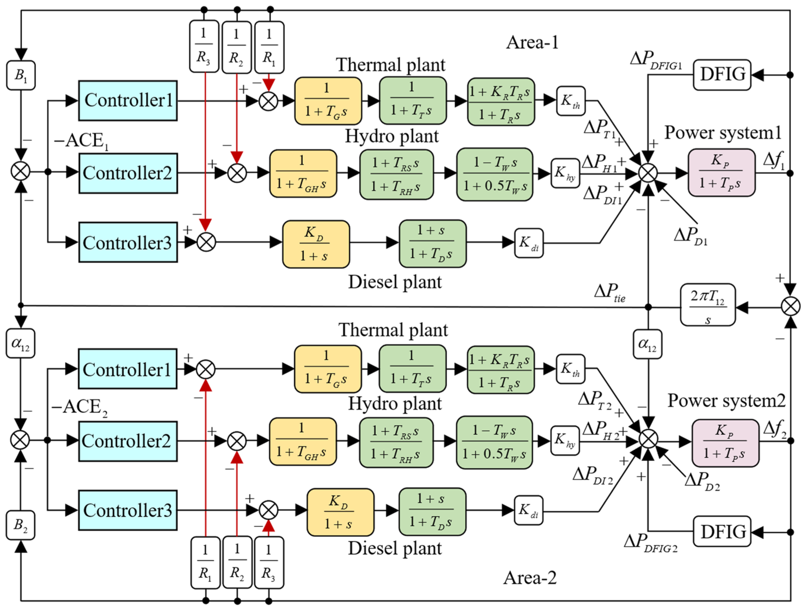
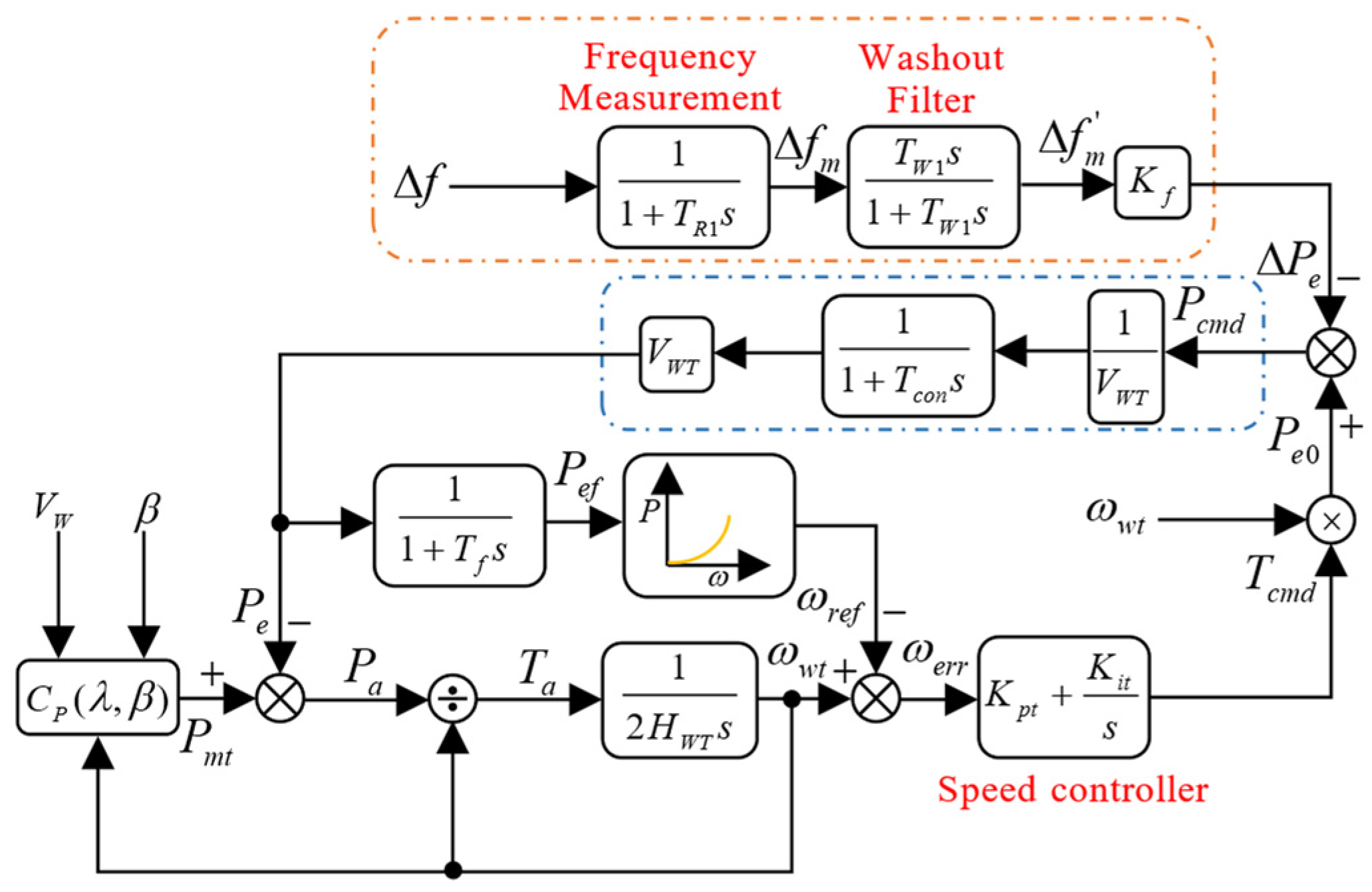
2. Systems Investigated

The model of the two-area interconnected power system adopted in this study is illustrated in Figure 1. In the given test system, each area contains a thermal unit, hydro plant, and diesel generator set with an integrated DFIG-driven wind energy conversion system, where the installed capacity of the wind turbines is 10% of the total installed capacity of the system. The synchronous unit output dominates the system frequency adjustment process. DFIG participates in part of the power system frequency adjustment through inertial response to reduce the synchronous frequency regulation pressure. With the fluctuation of load disturbance and wind power active output in the interconnected power system, the regional frequency of the power system constantly changes. In extreme circumstances, it could risk the security of the electrical system. As a result, the CPSOGSA method parameters optimize the CC-FOC of each area to ensure that the frequency ( Δ f 1 , Δ f 2 ) and the pull-line power deviation ( Δ P t i e ) of each area are within the legal bounds of the system. In addition, the following subsection discusses the mathematical model of DFIG used in the regional interconnection system. The system parameters involved are shown in Appendix A.

DFIG and Its Additional Frequency Response Model

The model structure of DFIG used in this study and its participation in the droop control principle of the system frequency response is shown in Figure 2. Among them, the output power of the wind turbine is closely related to the wind speed, and the relationship between the mechanical power of DFIG and the actual wind speed could be denoted by Equation (1).
P m = ( ρ A r 2 S N C p , o p t ) V w 3
where ρ is the density of air, S N represents the rated power of the wind turbine, A r is the wind turbine blade area, and V w represents the actual wind speed, C p , o p t is the optimal wind energy utilization factor.
The wind energy utilization factor C p of the wind turbine is given in Equation (2).
C p ( λ , β ) = i = 0 4 j = 0 4 α i , j β i λ j
where α i , j is the polynomial coefficient, β is the pitch angle, and λ is the blade tip speed ratio. λ is defined as shown in Equation (3).
λ = ω 0 R ω ω t V w
where ω w t is the DFIG rotor speed input, ω 0 is the DFIG rotor rated speed in m/s, and R is the wind turbine blade radius.
The relationship between the reference speed and the electromagnetic power of the wind turbine is given by
ω r e f = 0.67 P e f 2 + 1.42 P e f + 0.51
where P e f is the DFIG measured electrical power, ω r e f is the reference speed for maximum power tracking.
The additional frequency response of the wind turbine consists of three parts: frequency measurement module, washout filtering module, and droop control, where the transfer function of the frequency measurement module is given by
Δ f m = 1 1 + T R 1 s Δ f
washout filter module:
Δ f m = T w 1 s 1 + T w 1 s Δ f m
droop control:
Δ P e = K f Δ f m
where T R 1 is the frequency measurement module time gain, T W 1 is the washout filter gain factor, K f is the sag control gain, and Δ P e is the active power variation of the DFIG additional frequency response.

3. Cascade Fractional Order Controller Design

3.1. Implementation of Fractional Calculus

Fractional calculus is a non-integer order calculus, and the fractional order definition has several formulations in various viewpoints. The following equation introduces a unified fractional order calculus operator.
D m α γ = d α d t α α > 0 1 α = 0 α R γ m ( d τ ) α α < 0
where D is the fractional order calculus operator, m and γ are the up and down bounds of the calculus operator, respectively, and α denotes the order of the fractional order operator.
The most popular fractional-order calculus operator is the one defined by the Riemann–Liouville theorem. Equations (9) and (10) demonstrate the definitions of the integral operator and the calculus.
D m α γ f ( t ) = 1 Γ ( n α ) d n d t n γ m f ( τ ) ( t τ ) α n + 1 d τ , n - 1 < α < n n R
D m α γ f ( t ) = 1 Γ ( α ) γ m ( t τ ) α 1 f ( τ ) d τ
where n denotes the order of the calculus operator for fractional orders and Γ ( · ) is the Eulerian Gamma function.
While the fractional-order controller under the Riemann–Liouville definition can accurately calculate the fractional-order calculus value for a given signal, it is challenging to implement in a practical system. In contrast, the Oustaloup filter can approximate the fractional-order calculus operator well within a specific frequency interval ( ω L , ω H ) and at order N f .
s α ( d ω H b ) α ( d s 2 b ω H s d ( 1 α ) b s 2 + b ω H s + d α ) G p
G p , ω k , and ω k can then be calculated from Equations (12) and(13) as follows:
G p = k = N f N f s + ω k s + ω k
ω k = ( b ω H d ) α + 2 k 2 N f + 1 , ω k = ( b ω L d ) α 2 k 2 N f + 1
In the above Equation d = 9 , b = 10 , the frequency interval is 0.001 , 1000 , N f = 5 .

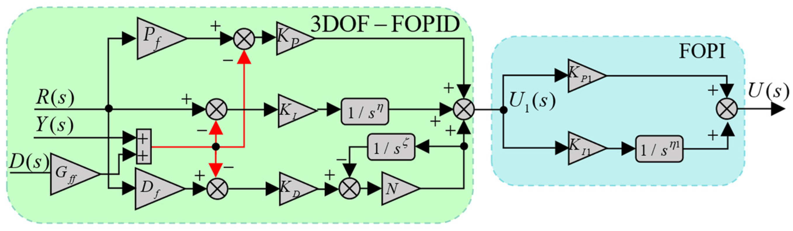
3.2. Cascade 3DOF-FOPID-FOPI Controller

In this study, a CC-FOC is devised to enhance the LFC efficiency of the interconnected system and reduce the system frequency changes brought on by load disturbances and wind fluctuations. The structure block diagram of the cascade controller is shown in Figure 3. The designed cascaded fractional order controller comprises two parts, a 3DOF-FOPID controller and a FOPI controller, connected by cascading.

3.2.1. 3DOF-FOPID Controller

The dynamic performance of the multi-degree-of-freedom controller facilitates better suppression of system oscillations. The 3DOF-FOPID controller, in its traditional form, consists of three parts, which serve to increase the closed-loop stability of the controller and reduce external disturbances through the closed-loop response. The following equation gives the output response of the 3DOF-FOPID controller.
U 1 ( s ) = P f K P + K I s η + D f K D s ζ ( N N + s ζ ) R ( s ) +   K P K I s η K D s ζ ( N N + s ζ ) Y ( s ) +   G f f K P K I s η G f f K D s ζ ( N N + s ζ ) D ( s )
where η , ζ , are the integral gain and differential gain.

3.2.2. FOPI Controller

U ( s ) = K P 1 + K I 1 s η 1 U 1 ( s )
The linear inequality for the parameter boundaries of the cascade controller is given by
K P min K P K P max , K P 1 min K P 1 K P 1 max K I min K I K I max , K I 1 min K I 1 K I 1 max K D min K D K D max , η min η η max , η 1 min η 1 η 1 max ζ min ζ ζ max , P f min P f P f max , D f min D f D f max G f f min G f f G f f max , N min N N max
where min is the minimum value of the cascade controller gain and max is the maximum value of the cascade controller gain. For the new cascade controller, there is no definite method to determine these values at the beginning of the controller design [33]. To enhance the reliability of the interconnected area power system and obtain better parameter optimization, the range of controller gains K P , K I , K D , K P 1 , and K I 1 take values in the range of 0 to 2. The values of η , η 1 , ζ , and G f f are in the range of 0 to 1. P f and D f take values in the range of 0 to 3. The value range of N is from 10 to 200.

4. The Proposed CPSOGSA Algorithm

This section will first discuss the particle swarm optimization (PSO) algorithm and the gravitational search algorithm (GSA) that make up the CPSOGSA algorithm, explain the principles and mathematical expressions of the two algorithms, and then introduce the chaotic mapping and its parameter search process in the CPSOGSA algorithm in detail.

4.1. Particle Swarm Optimization

Based on the biological behavior of a flock of birds seeking food, Kennedy et al. introduced the PSO algorithm, an intelligent optimization technique [34]. The core idea of the algorithm is to use particles to mimic individual birds, with the position of each particle being a potential solution to the problem. Each particle in the current particle swarm maintains its optimal solution information during the search process, while the particle swarm maintains the population’s optimal solution information. The velocity and position of each particle in the current particle swarm are updated continuously throughout the optimization solution process. The iterative search procedure is halted, and the optimum solution is produced when the predetermined number of iterations or population ideal solution accuracy is obtained. The particle of the particle swarm updates for location and velocity are provided by
v i ( t + 1 ) = w v i ( t ) + c 1 · r a n d · ( p b e s t i p i ( t ) ) + c 2 · r a n d · ( g b e s t i p i ( t ) )
p i ( t + 1 ) = p i ( t ) + v i ( t + 1 )
where v i ( t ) and p i ( t ) are the velocity and position of particle i , respectively, c 1 and c 2 are the particle’s population learning factor as well as its learning factor, respectively, w represents the inertia factor, and r a n d represents the random number with the interval at [0, 1].

4.2. Gravitational Search Algorithm

The design idea of GSA is derived from the law of gravitation in physics [35]. In GSA, the positions of particles orbiting in space are considered solutions to the optimization problem, and each particle interacts with the other through universal gravity. The position of that particular particle is the best answer to the optimization issue because, under the influence of gravity, all particles will eventually move toward the individual particle with an enormous mass. Assuming that there are N individuals in the initial population of GSA, the position of the i th individual in space can be defined as shown in Equation (19).
p i = ( p 1 1 , p i c , p i n ) i = 1 , 2 , N
where p i is the position of the ith particle in the cth dimension and n is the specified dimension of the ith particle. At the t moment, the mass of the particle is given by
m i ( t ) = f i t i ( t ) w o r s t ( t ) b e s t ( t ) w o r s t ( t )
M i ( t ) = m i ( t ) j = 1 N m j ( t )
where f i t i ( t ) is the fitness value of particle i at time t ; m i ( t ) is the mass of particle i at time t ; b e s t ( t ) , w o r s t ( t ) are the optimal fitness value and the worst fitness value of all particles at time t , respectively, and are defined accordingly as follows:
b e s t ( t ) = min f i t i ( t ) i 1 , 2 , N
w o r s t ( t ) = max f i t i ( t ) i 1 , 2 , N
This paper is a minimization problem for the optimal control of the system load frequency, so the calculation method of this adaptation degree is used.
At the moment t , the universal gravitational force between the particle i and the particle j in the c th dimension is
F i j c = G ( t ) M i ( t ) M j ( t ) R i j ( t ) + ε ( p j c ( t ) p i c ( t ) )
where G ( t ) and R i j ( t ) are the universal gravitational constant at the moment of t and the Euclidean distance between particle i and particle j , respectively, and ε is a very small constant.
Then the total force exerted on particle i is given by
F i c ( t ) = j = 1 , j i N r a n d j F i j c ( t )
where r a n d j represents a random number of [0, 1].
In each iteration of the GSA algorithm, each particle updates its next-generation velocity v i c ( t + 1 ) and position p i c ( t + 1 ) according to the acceleration a i c ( t ) , which is calculated as follows:
a i c ( t ) = F i c ( t ) / M i ( t )
v i c ( t + 1 ) = r a n d j v i c ( t )
p i c ( t + 1 ) = p i c ( t ) + v i c ( t + 1 )
GSA will update the particle velocity and position throughout the optimization search process and then calculate the gravitational force of each particle. After several iterations, the individual particles with higher masses will get better positions and keep gathering other particles. The optimal solution will be output when the number of iterations reaches a predetermined value.

4.3. Improved PSOGSA Algorithm under Chaotic Map Optimization (CPSOGSA)

The hybrid PSOGSA algorithm comprises two parts, PSO and GSA, and its equations of motion are shown in Equations (29) and (30).
v i ( t + 1 ) = w v i ( t ) + c 1 · r a n d · ( p b e s t i p i ( t ) ) + c 2 · r a n d · ( g b e s t i p i ( t ) )
p i ( t + 1 ) = p i ( t ) + v i ( t + 1 )
Chaos, as a nonlinear system with complex behavior and random characteristics, is very sensitive to initial conditions. Due to its disorderly and ergodic characteristics, chaos can be traversed through all the state points in the chaotic area in a finite time. Therefore, the hybrid PSOGSA algorithm is optimized using the chaotic mapping method to improve the convergence speed of the algorithm while preventing the particle position from converging and jumping out of the optimal local solution in time. Therefore, this paper adopts the method of chaotic mapping instead of random numbers to calculate the total force applied to the particles, thus improving the GSA algorithm’s local search ability and convergence speed.
The total force of particle i using the chaotic mapping method is calculated as shown in Equation (31).
F i c ( t ) = j ( k ) b e s t , j i C ( t ) F i j c ( t )
where C ( t ) is the value of the function generated using a one-dimensional chaotic mapping. Table 1 shows the ten functions used to generate chaotic mappings in this paper [36,37], none of which have random numbers and do not generate values between 0 and 1 but are simply normalized to the same scale. Figure 4 shows the chaotic curves generated using the chaotic mapping function, which changes according to the number of iterations. Simulation tests of the PSOGSA algorithm optimized by these 10 chaotic map mapping functions are conducted in the literature [31]. The simulation results show that the PSOGSA algorithm under Sinusoidal chaotic map optimization has the best convergence speed and smaller fitness values. Therefore, Sinusoidal chaotic maps are chosen to optimize the PSOAGSA algorithm in this study. In addition, the parameter settings of the CPSOGSA algorithm in this study are given in Appendix A.
The time multiplied squared error (ITSE) is used in this study as the performance indicator and goal function for assessing the LFC of the system, and CPSOGSA is used to tune and optimize the relevant CC-FOC system parameters. The system objective function is shown in Equation (32).
J = I T S E = min 0 T ( Δ f 1 2 + Δ f 2 2 + Δ P t i e 2 ) d t
In comparing the controller performance, the CPSOGSA algorithm will be used to optimally iterate each controller parameter with Equation (32) as the objective function. The algorithm’s optimization search process for the controller parameters is shown in Figure 5.

5. Simulation Analysis

As illustrated in Figure 1, the frequency model of the two-area interconnected power system containing DFIG is built based on the R2021b MATLAB/SIMULINK environment in this study, and the proposed cascaded 3DOF-FOPID-FOPI controller is simulated and verified. This section will use load perturbation and wind speed fluctuation to simulate the interconnected electrical system. The LFC performance of several controllers is then compared, and the robustness of the CC- FOC is evaluated. In addition, to illustrate the excellent performance of the CPSOGSA algorithm on parameter search, the parameters of the CC-FOC in the system will be iteratively searched for using DE, PSO, GSA, CHGSA, and CPSOGSA, respectively. Whereas with the CPSOGSA algorithm, the number of particles is fixed at 50, and the procedure has 100 iterations overall.

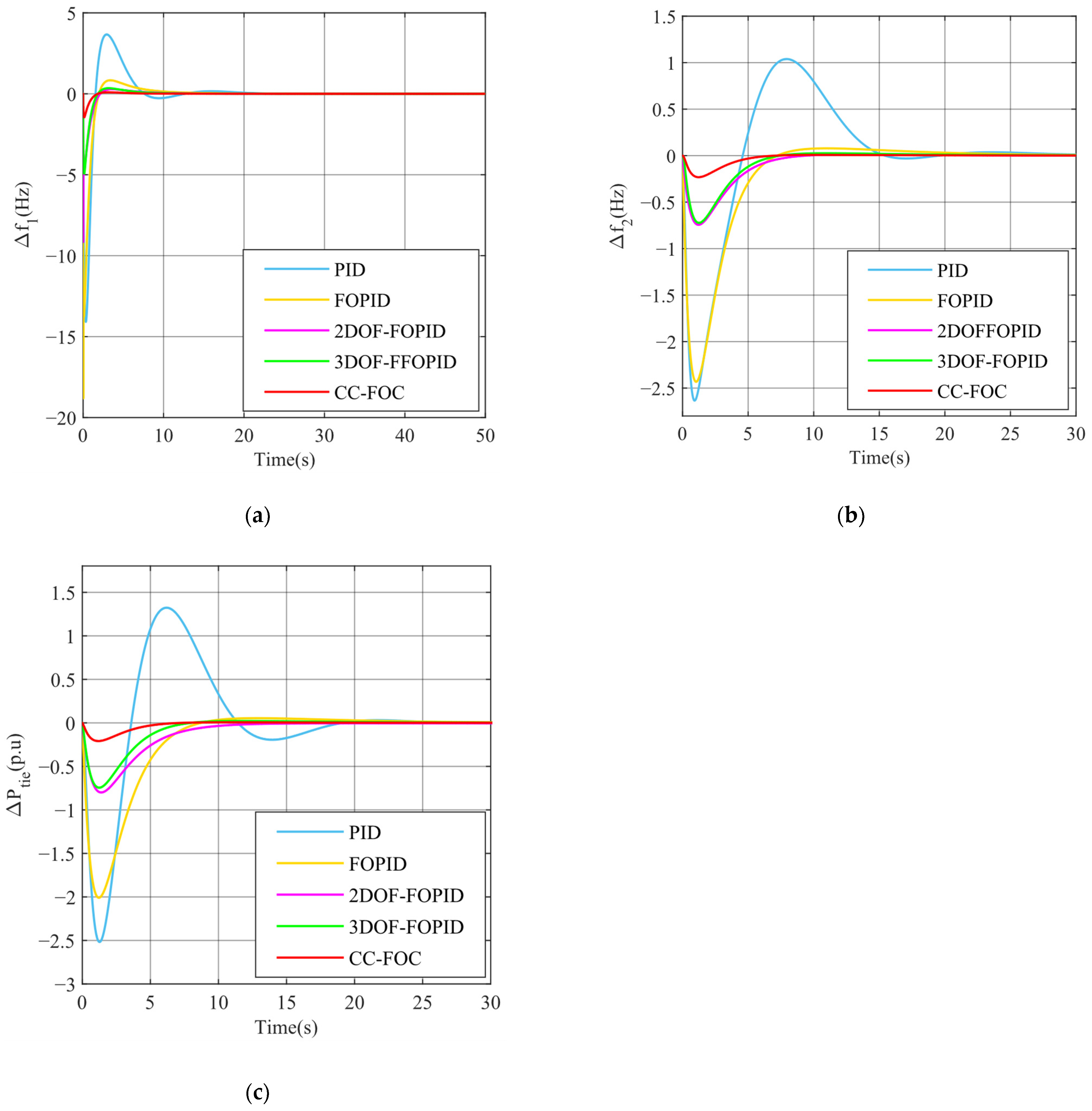
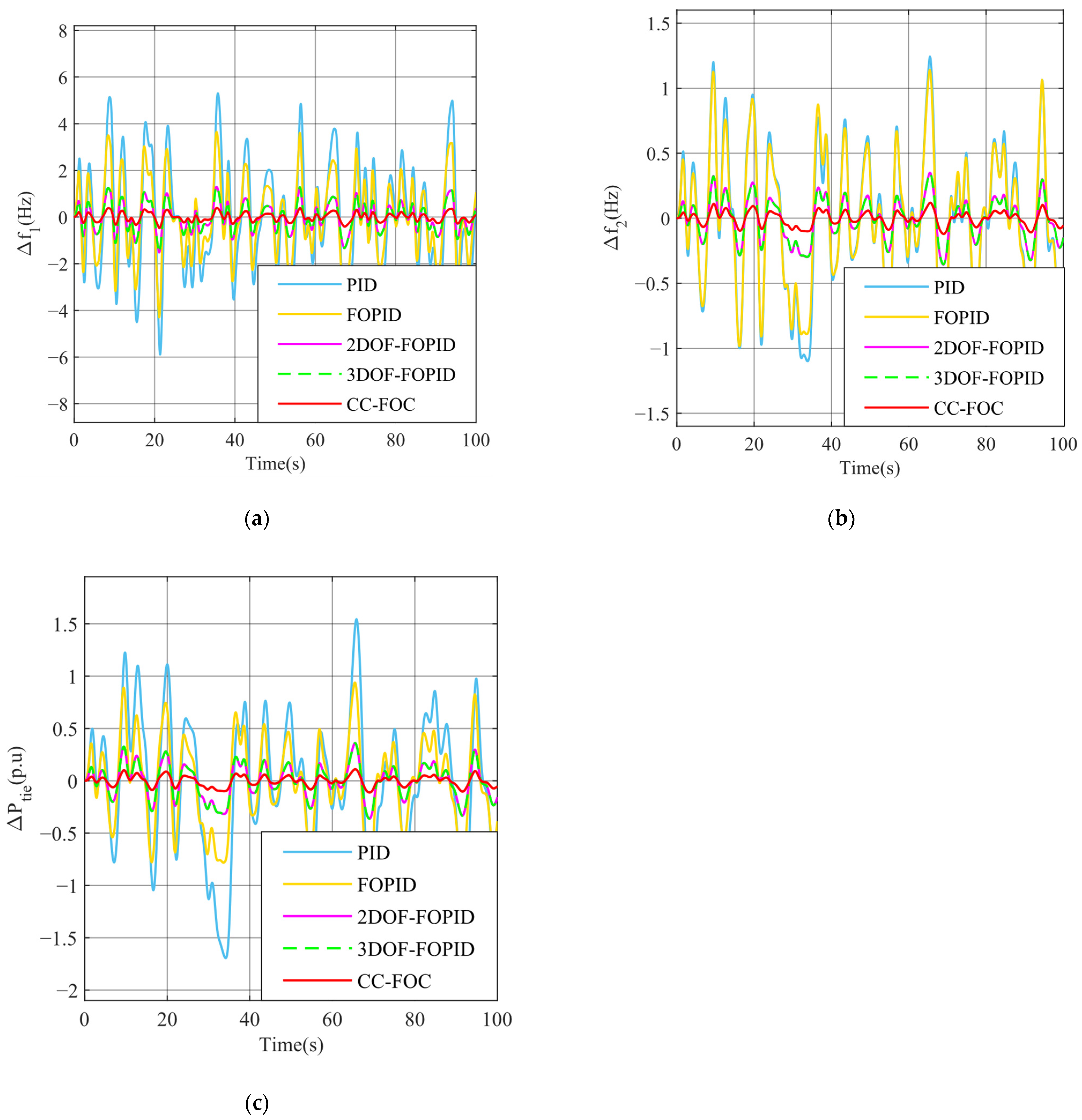
5.1. Scenario 1 Effect of Different Load Perturbations

In this subsection, two operating conditions are included, the first is a +2% load disturbance in area 1 of the interconnected regional system at t = 0 s, and the second is a +2% load disturbance and a +4% load perturbation in areas 1 and 2 of the interconnected regional system at t = 0 s, respectively. The gains of the cascaded 3DOF-FOPID-FOPI controller, 2DOF-FOPID controller, FOPID controller, and PID controller are optimized based on the CPSOGSA algorithm to compare the control performance of each controller under load perturbation.
Under a +2% load perturbation in area 1, Table 2 illustrates the optimal gain for each controller in the regionally interconnected system based on the ITSE fitness function. Figure 6 and Figure 7 illustrate the response curves of the system frequency deviation and contact line power deviation under different load disturbance conditions, respectively. Table 3 shows the values of undershoot (US), overshoot (OS), settling time ( T s ), and objective function (ITSE) for the system under different controllers. Settling time is defined as a tolerance range of 0.002%. According to Table 3, when the controller gains are optimized and the CPSOGSA algorithm is used, the cascaded 3DOF-FIPID-FOPI controller performs considerably outperforming the other four controllers. In the case of +2% load perturbation in area 1, for the maximum drop US of Δ f 1 , the CC-FOC reduces 70.41%, 84.07%, 92.29%, and 89.71% compared to the 3DOF-FOPID controller, 2DOF-FOPID controller, FOPID controller, and PID controller, respectively. In addition, for the maximum overshoot OS of Δ f 1 , the CC-FOC reduces 72.33%, 66.43%, 88.53%, and 96.80% compared to the 3DOF-FOPID controller, 2DOF-FOPID controller, FOPID controller, and PID controller, respectively. For the settling time T s of Δ f 1 , the CC-FOC well reduces the settling time of frequency recovery under the specification of the objective function. CC-FOC decreases the settling time of frequency recovery by 76.26%, 76.70%, 85.33%, and 88.22%.

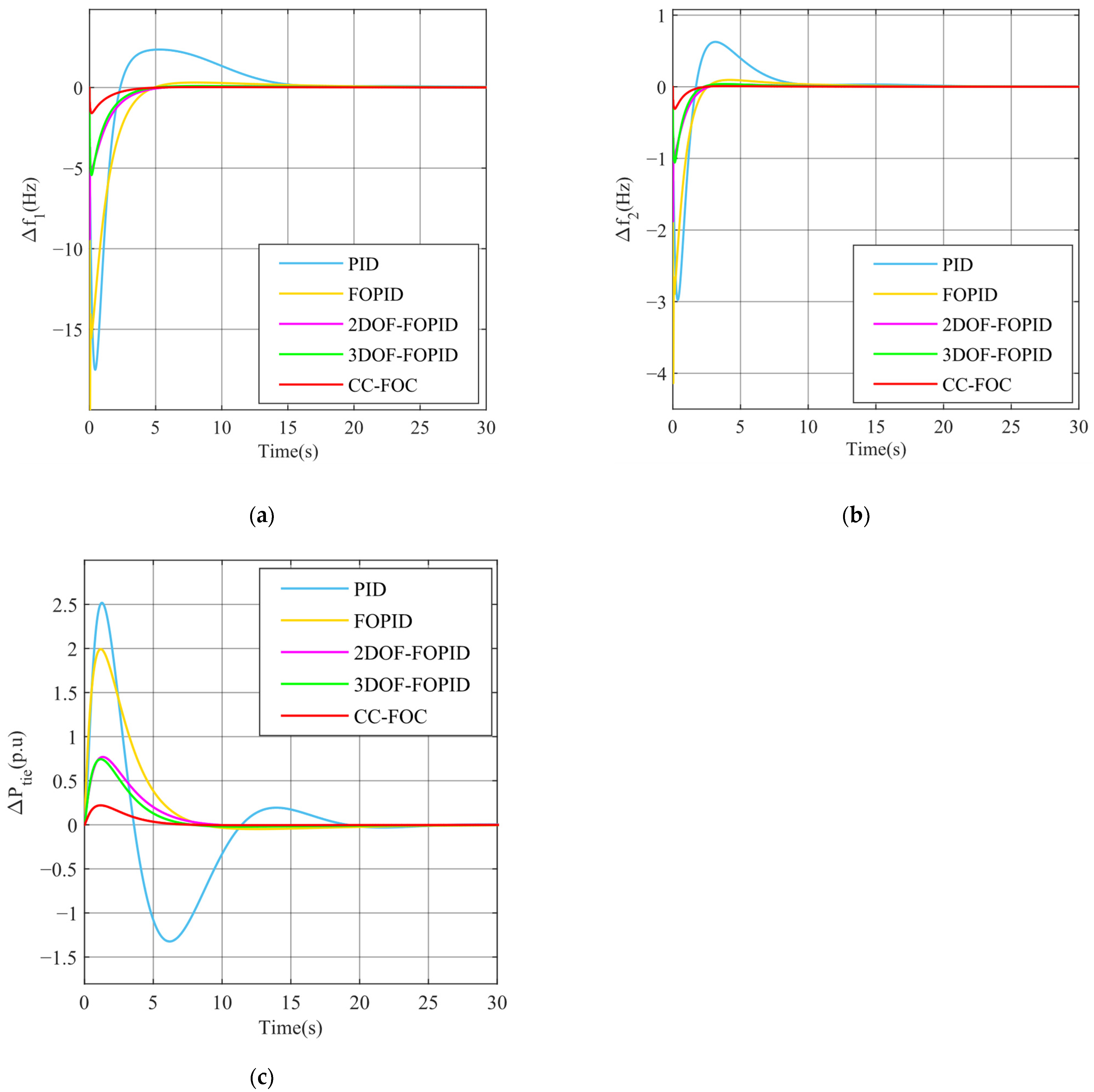
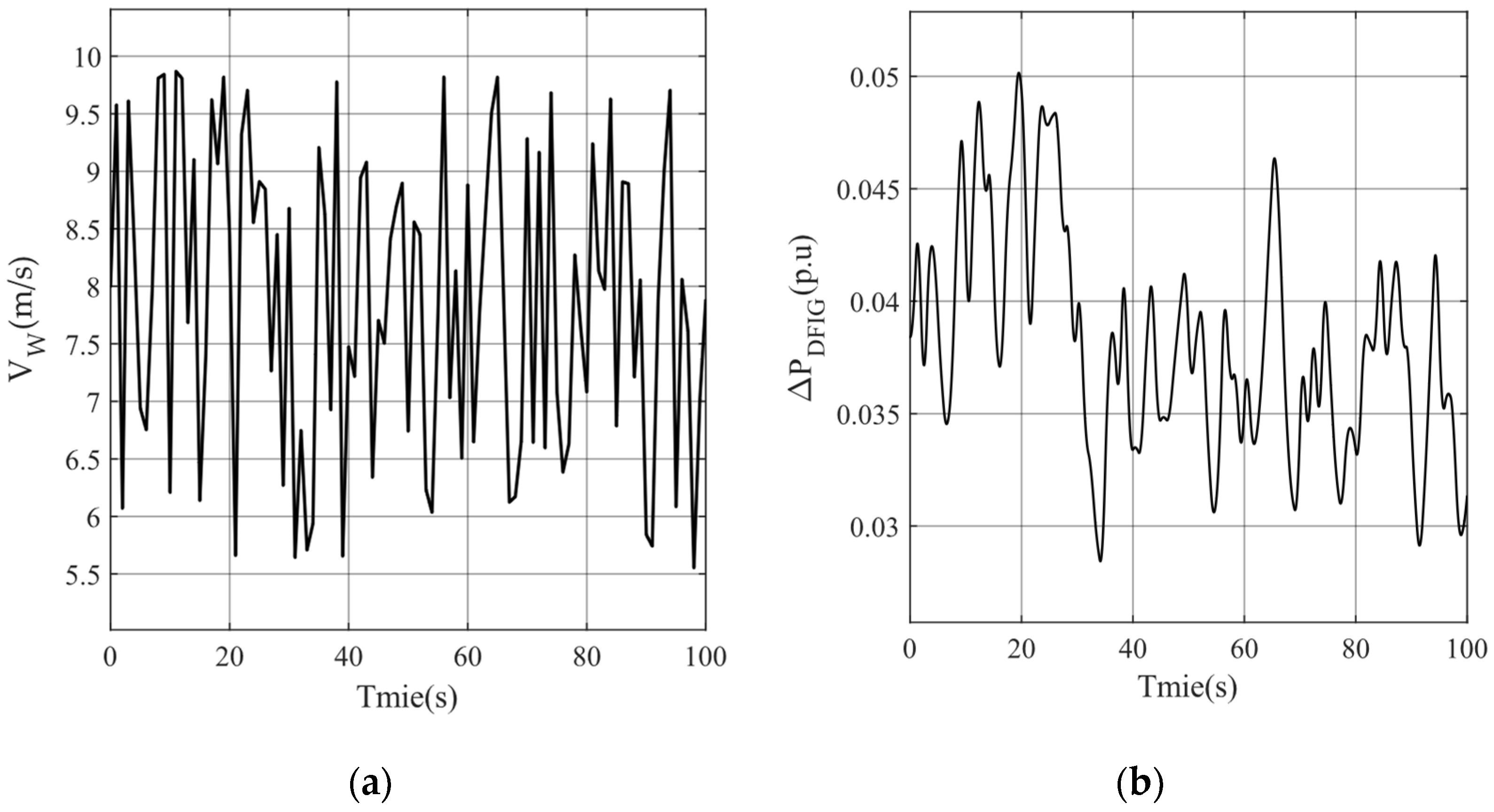
5.2. Scenario 2 Wind Speed Fluctuations

The frequency stabilization of the connected regional system comprising DFIG is simulated and confirmed under stochastic wind speed conditions to validate the control performance of the cascade controller in a more realistic setting. The random wind speed of the wind turbine in area 1 is illustrated in Figure 8a, and the resulting active output of the DFIG is shown in Figure 8b. Under the influence of stochastic wind speed, the zone frequency and contact line power of the interconnected power system also change, and the corresponding dynamic response curves are shown in Figure 9. The LFC performance of the CPSOGSA-optimized cascade controller is much better than the other four controllers, as illustrated by the variation curves of system frequency and contact line power under random wind speed fluctuations in area 1.

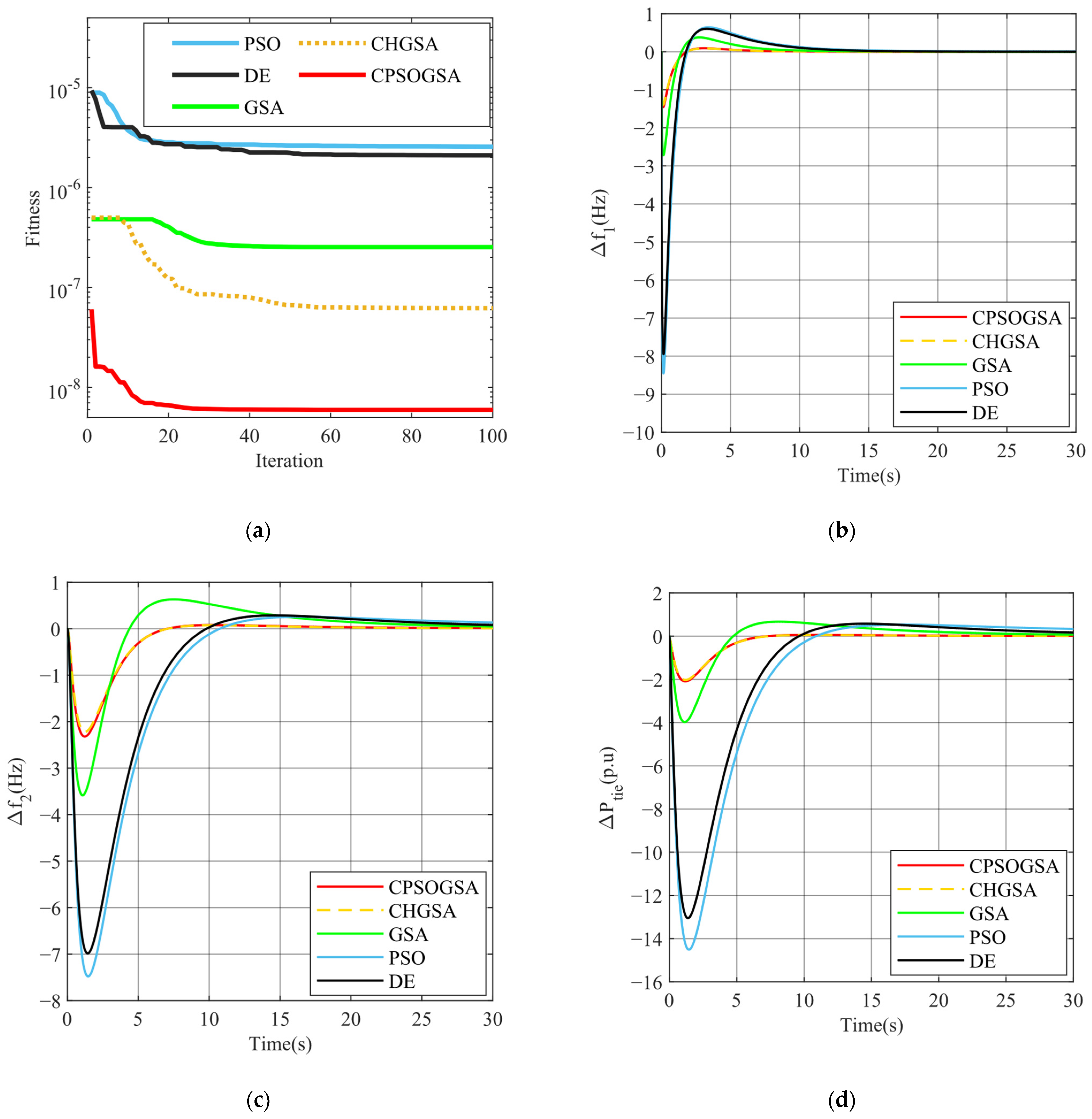
5.3. Scenario 3 Comparison of Different Optimization Algorithms

The primary purpose of this subsection is to illustrate the excellence of the CPSOGSA algorithm in optimizing the cascade controller parameters. For this purpose, CPSOGSA is compared with four other algorithms. Individual algorithms are used to optimize all parameters of the proposed cascade controller in the presence of the same operating disturbance.
The iterative process of the various algorithms is reflected in Figure 10a, and it can be seen that CPSOGSA converges faster than the other four algorithms and has a smaller fitness value, i.e., the controller parameters found are better. However, the convergence speed and fitness value of PSO and GSA could be more satisfactory and even fall into the local optimum. Figure 10b–d show the frequency variation curves of the regional interconnected power system and the dynamic response curves of the contact line power deviation obtained by different algorithms for the cascade controller when the interconnected regional system faces the same disturbances. From the dynamic response results of the system, it is known that the cascade controller under CPSOGSA optimization exhibits better system frequency control capability.

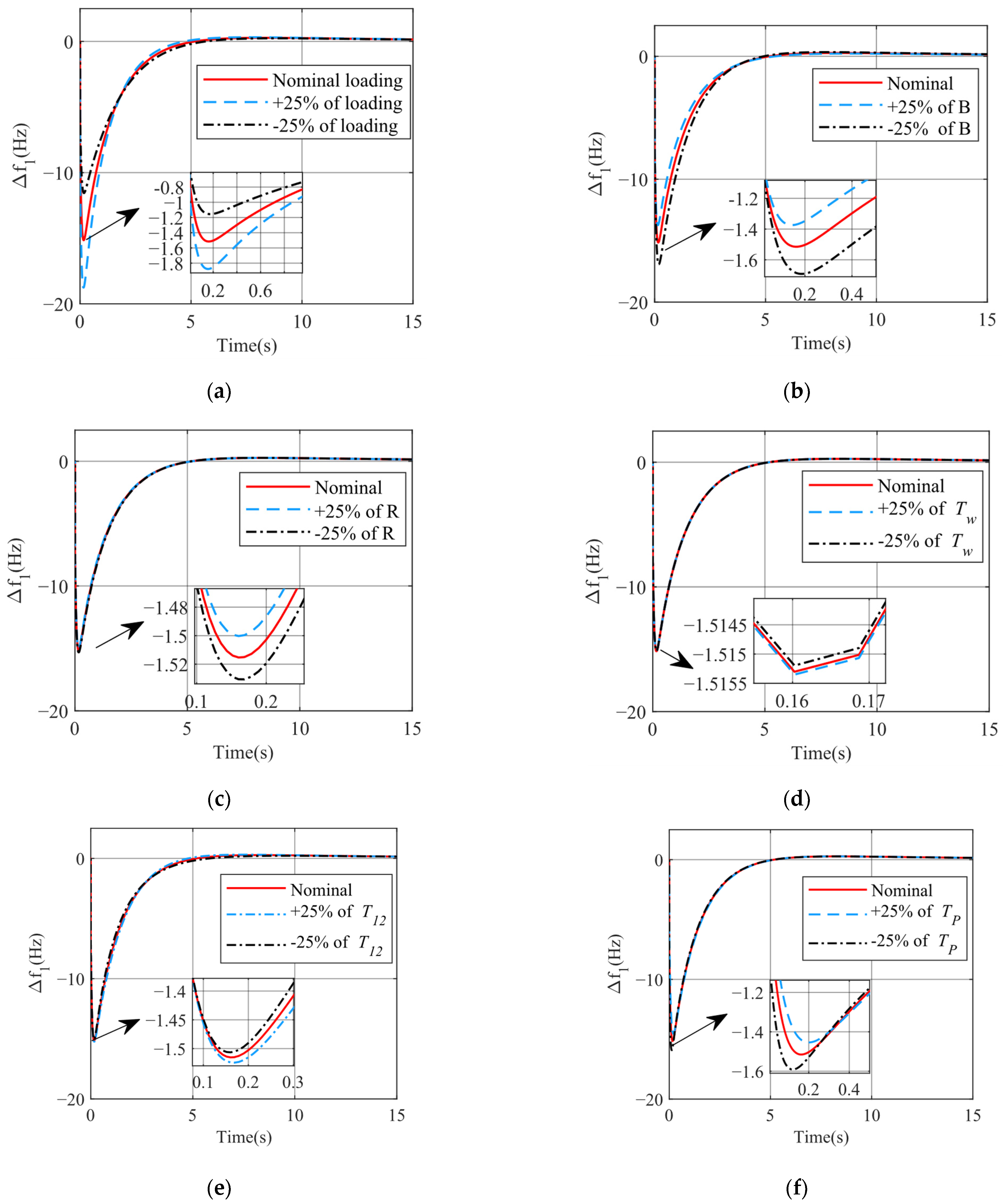
5.4. Scenario 4 Load Perturbation and Internal Parameter Changes

The robustness of the load frequency controller is important for the system, so this subsection will reflect the robustness of the proposed cascade controller by varying the load perturbation and system parameters in a simulation environment for sensitivity analysis. The load perturbation circumstances and system parameters are altered between +25% and −25% of their nominal values in the simulated evaluation of the controller resilience. Figure 11 shows the frequency dynamic response of area 1 under varying load disturbance and system parameters such as the time constant of the hydropower plant ( T w ), frequency bias parameter ( B ), droop governor characteristic ( R ), stiffness coefficient ( T 12 ), and power system time constant ( T P ). From Figure 11a,b, we can learn that the load disturbance and the system parameter B have some influence on the stabilization of the system frequency, among which the influence of the load disturbance change is the most obvious, but the LFC performance of the system is still very good. The impact of the change of other system parameters in the range of ± 25 % on the system frequency deviation is negligible, which fully illustrates the robustness of the proposed cascade controller.
Table 4 gives the US/OS and settling time of the frequency deviation and tie-line deviation for areas 1 and 2 under load perturbation and different system parameter changes. Taking B as an example, with a +25% increase in B , the US of Δ f 1 , Δ f 2 , and Δ P t i e only changes by 8.61%, 16.52%, and 7.17%, the overshoot of Δ f 1 , Δ f 1 , and Δ P t i e only changed by 9.38%, 20%, and 0, respectively, and the settling time of Δ f 1 , Δ f 1 , and Δ P t i e only changed by 1.276%, 23.86%, and 7.68%, respectively. All the results illustrate the excellent robustness of CC-FOC under CPSOGSA algorithm optimization.

6. Conclusions and Future Work

This paper proposes a cascaded 3DOF-FOPD-FOPI controller for the LFC problem of a two-area interconnected power system integrated with DFIG. The parameters of the cascaded controller are optimized under the objective function of ITSE using the CPSOGSA algorithm. Simulation results show that the cascade controller optimized with the CPSOGSA algorithm provides better control output performance in the LFC of interconnected power systems than other controllers. The suggested cascade controller can reduce frequency stabilization time and overshoot and undershoot for conventional load disturbances and wind turbine output power variations caused by wind speed fluctuations. In addition, the CPSOGSA algorithm effectively optimizes the controller gain. It can converge quickly and find the optimal optimized gain even in a state with many cascade controller parameters. The sensitivity analysis of varying load perturbations and system parameters also illustrates the robustness of the cascade controller.
In future work, optimization of the control structure of the cascaded fractional-order controller will be considered to reduce the number of controller parameters while ensuring the control performance, as well as to analyze the impact of wind power entry on the inertia aspects of the power system.

Author Contributions

Conceptualization, S.X.; methodology, S.X. and Y.Z.; software, S.X.; validation, Y.Z. and F.Y.; formal analysis, S.X.; investigation, S.X.; resources, Y.Z.; data curation, S.X. and J.Q.; writing—original draft preparation, S.X.; writing—review and editing, S.X. and Y.Z.; visualization, Y.L.; supervision, S.X.; project administration, S.X.; funding acquisition, Y.Z.; All authors have read and agreed to the published version of the manuscript.

Funding

This research was funded by the National Natural Science Foundation of China (No. 52079059 and 52269020).

Data Availability Statement

Not applicable.

Conflicts of Interest

The authors declare no conflict of interest.

Abbreviations

CC-FOCCascade fractional-order controller
CPSOGSAImproved particle swarm optimization and gravitational search algorithm under chaotic map optimization
DEDifferential evolution
DFIGDoubly-fed induction generator
FOPIFractional-order proportional-integral
GSAGravitational search algorithm
ITSETime multiplied squared error
LFCLoad frequency control
PSOParticle swarm optimization
PIDProportional-integral-differential
2DOF-FOPIDTwo-degree-of-freedom fractional-order proportional-integral-differential
3DOF-FOPIDThree-degree-of-freedom fractional-order proportional-integral-differential

Appendix A

Parameters of the two-area 1nterconnection system
T G = 0.08   s , T T = 0.3   s , T r = 10   s , K r = 0.3   s , T G H = 0.2   s , T R H = 28.75   s , T R S = 5   s , T W = 1   s , K D = 16.5 , T D = 0.025   s , T P = 11.49   s , K P = 68.9566   Hz / pu , R i = 2.4   Hz / pu , K t h = 0 . 543478 , K h y = 0 . 326084 , K d i = 0 . 130438 , T 12 = 0 . 0433   s , B 1 , B 2 = 0 . 4312   s , α 12 = 1 .
B 1 , B 2 , frequency bias parameters; T G , governor time constant of thermal unit; T T , steam turbine time constant of thermal unit; T r , steam turbine reheat time constant; K r , steam turbine reheat gain constant; T G H , governor time constant of hydro unit; T R H , hydro turbine speed governor transient time droop constant; T R S , hydro turbine speed governor reset time; T W , water flow inertia time constant; K D , the gain of the diesel generator unit; T D , time constant of the diesel generator unit; T P , power system time constant; K P , power system gain; T 12 , synchronization coefficient; R i , governor regulation parameter; A C E , area control error.
Parameters of DFIG
T f = 5   s , T c o n = 0.02   s , ω 0 = 1.33   rad / s , K p t = 3   s , K i t = 0.6   s , V W T = 1   pu , H W T = 5.19   s , T R 1 = 0.2   s , T W 1 = 6   s , R = 52   m , 0.5 ρ A r / S N = 0.00145 .
Parameters of CPSOGSA
c 1 = 1 . 4962 , c 2 = 1 . 4962 , w = 0 . 7298 , N = 50 , I t e r a t i o n = 100 .

References

  1. Olabi, A.G.; Abdelkareem, M.A. Renewable energy and climate change. Renew. Sustain. Energy Rev. 2022, 158, 112111. [Google Scholar] [CrossRef]
  2. Cao, M.; Xu, Q.; Qin, X.; Cai, J. Battery energy storage sizing based on a model predictive control strategy with operational constraints to smooth the wind power. Int. J. Electr. Power Energy Syst. 2020, 115, 105471. [Google Scholar] [CrossRef]
  3. Tavakkoli, M.; Fattaheian-Dehkordi, S.; Pourakbari-Kasmaei, M.; Liski, M.; Lehtonen, M. An Approach to Divide Wind Power Capacity Between Day-Ahead Energy and Intraday Reserve Power Markets. IEEE Syst. J. 2022, 16, 1123–1134. [Google Scholar] [CrossRef]
  4. Du, M.; Niu, Y.; Hu, B.; Zhou, G.; Luo, H.; Qi, X. Frequency regulation analysis of modern power systems using start-stop peak shaving and deep peak shaving under different wind power penetrations. Int. J. Electr. Power Energy Syst. 2021, 125, 106501. [Google Scholar] [CrossRef]
  5. Bevrani, H.; Golpîra, H.; Messina, A.R.; Hatziargyriou, N.; Milano, F.; Ise, T. Power system frequency control: An updated review of current solutions and new challenges. Electr. Power Syst. Res. 2021, 194, 107114. [Google Scholar] [CrossRef]
  6. Khalid, J.; Ramli, M.A.M.; Khan, M.S.; Hidayat, T. Efficient Load Frequency Control of Renewable Integrated Power System: A Twin Delayed DDPG-Based Deep Reinforcement Learning Approach. IEEE Access 2022, 10, 51561–51574. [Google Scholar] [CrossRef]
  7. Mi, Y.; Chen, B.; Cai, P.; He, X.; Liu, R.; Yang, X. Frequency control of a wind-diesel system based on hybrid energy storage. Prot. Control Mod. Power Syst. 2022, 7, 31. [Google Scholar] [CrossRef]
  8. Kalyan, C.N.S.; Goud, B.S.; Reddy, C.R.; Bajaj, M.; Sharma, N.K.; Alhelou, H.H.; Siano, P.; Kamel, S. Comparative Performance Assessment of Different Energy Storage Devices in Combined LFC and AVR Analysis of Multi-Area Power System. Energies 2022, 15, 629. [Google Scholar] [CrossRef]
  9. Mi, Y.; Hao, X.Z.; Liu, Y.J.; Fu, Y.; Wang, C.S.; Wang, P.; Loh, P.C. Sliding mode load frequency control for multi-area time-delay power system with wind power integration. IET Gener. Transm. Distrib. 2017, 11, 4644–4653. [Google Scholar] [CrossRef]
  10. Fan, W.; Hu, Z.; Veerasamy, V. PSO-Based Model Predictive Control for Load Frequency Regulation with Wind Turbines. Energies 2022, 15, 8219. [Google Scholar] [CrossRef]
  11. Vafamand, N.; Arefi, M.M.; Asemani, M.H.; Dragičević, T. Decentralized Robust Disturbance-Observer Based LFC of Interconnected Systems. IEEE Trans. Ind. Electron. 2022, 69, 4814–4823. [Google Scholar] [CrossRef]
  12. Adibi, M.; Woude, J.v.d. Secondary Frequency Control of Microgrids: An Online Reinforcement Learning Approach. IEEE Trans. Autom. Control 2022, 67, 4824–4831. [Google Scholar] [CrossRef]
  13. Ali, M.; Kotb, H.; Aboras, K.M.; Abbasy, N.H. Design of Cascaded PI-Fractional Order PID Controller for Improving the Frequency Response of Hybrid Microgrid System Using Gorilla Troops Optimizer. IEEE Access 2021, 9, 150715–150732. [Google Scholar] [CrossRef]
  14. Rostami, Z.; Ravadanegh, S.N.; Kalantari, N.T.; Guerrero, J.M.; Vasquez, J.C. Dynamic Modeling of Multiple Microgrid Clusters Using Regional Demand Response Programs. Energies 2020, 13, 4050. [Google Scholar] [CrossRef]
  15. Khadanga, R.K.; Nayak, S.R.; Panda, S.; Das, D.; Prusty, B.R.; Sahu, P.R. A Novel Optimal Robust Design Method for Frequency Regulation of Three-Area Hybrid Power System Utilizing Honey Badger Algorithm. Int. Trans. Electr. Energy Syst. 2022, 2022, 6017066. [Google Scholar] [CrossRef]
  16. Patan, M.K.; Raja, K.; Azaharahmed, M.; Prasad, C.D.; Ganeshan, P. Influence of Primary Regulation on Frequency Control of an Isolated Microgrid Equipped with Crow Search Algorithm Tuned Classical Controllers. J. Electr. Eng. Technol. 2021, 16, 681–695. [Google Scholar] [CrossRef]
  17. Chen, G.; Li, Z.; Zhang, Z.; Li, S. An Improved ACO Algorithm Optimized Fuzzy PID Controller for Load Frequency Control in Multi Area Interconnected Power Systems. IEEE Access 2020, 8, 6429–6447. [Google Scholar] [CrossRef]
  18. Kamarposhti, M.A.; Shokouhandeh, H.; Alipur, M.; Colak, I.; Zare, H.; Eguchi, K. Optimal Designing of Fuzzy-PID Controller in the Load-Frequency Control Loop of Hydro-Thermal Power System Connected to Wind Farm by HVDC Lines. IEEE Access 2022, 10, 63812–63822. [Google Scholar] [CrossRef]
  19. Tabak, A. Fractional order frequency proportional-integral-derivative control of microgrid consisting of renewable energy sources based on multi-objective grasshopper optimization algorithm. Trans. Inst. Meas. Control 2021, 44, 378–392. [Google Scholar] [CrossRef]
  20. Ebrahim, M.A.; Becherif, M.; Abdelaziz, A.Y. PID-/FOPID-based frequency control of zero-carbon multisources-based interconnected power systems underderegulated scenarios. Int. Trans. Electr. Energy Syst. 2021, 31, e12712. [Google Scholar] [CrossRef]
  21. Agwa, A.M.; Abdeen, M.; Shaaban, S.M. Optimal FOPID Controllers for LFC Including Renewables by Bald Eagle Optimizer. CMC-Comput. Mater. Contin. 2022, 73, 5525–5541. [Google Scholar] [CrossRef]
  22. Pahadasingh, S.; Jena, C.; Panigrahi, C.K. Load Frequency Control Incorporating Electric Vehicles Using FOPID Controller with HVDC Link. In Proceedings of the Innovation in Electrical Power Engineering, Communication, and Computing Technology, Singapore, 22 February 2020; pp. 181–203. [Google Scholar]
  23. Mohapatra, T.K.; Dey, A.K.; Sahu, B.K. Employment of quasi oppositional SSA-based two-degree-of-freedom fractional order PID controller for AGC of assorted source of generations. IET Gener. Transm. Distrib. 2020, 14, 3365–3376. [Google Scholar] [CrossRef]
  24. Nayak, J.R.; Shaw, B.; Sahu, B.K. Implementation of hybrid SSA-SA based three-degree-of-freedom fractional-order PID controller for AGC of a two-area power system integrated with small hydro plants. IET Gener. Transm. Distrib. 2020, 14, 2430–2440. [Google Scholar] [CrossRef]
  25. Sahu, P.C.; Prusty, R.C.; Panda, S. Active power management in wind/solar farm integrated hybrid power system with AI based 3DOF-FOPID approach. Energy Sources Part A: Recovery Util. Environ. Eff. 2021, 1–21. [Google Scholar] [CrossRef]
  26. Ali, M.; Kotb, H.; Kareem AboRas, M.; Nabil Abbasy, H. Frequency regulation of hybrid multi-area power system using wild horse optimizer based new combined Fuzzy Fractional-Order PI and TID controllers. Alex. Eng. J. 2022, 61, 12187–12210. [Google Scholar] [CrossRef]
  27. Guha, D.; Roy, P.K.; Banerjee, S. Equilibrium optimizer-tuned cascade fractional-order 3DOF-PID controller in load frequency control of power system having renewable energy resource integrated. Int. Trans. Electr. Energy Syst. 2021, 31, e12702. [Google Scholar] [CrossRef]
  28. Barakat, M. Novel chaos game optimization tuned-fractional-order PID fractional-order PI controller for load–frequency control of interconnected power systems. Prot. Control Mod. Power Syst. 2022, 7, 16. [Google Scholar] [CrossRef]
  29. Choudhary, R.; Rai, J.N.; Arya, Y. Cascade FOPI-FOPTID controller with energy storage devices for AGC performance advancement of electric power systems. Sustain. Energy Technol. Assess. 2022, 53, 102671. [Google Scholar] [CrossRef]
  30. Guha, D.; Roy, P.K.; Banerjee, S. Frequency Control of a Wind-diesel-generator Hybrid System with Squirrel Search Algorithm Tuned Robust Cascade Fractional Order Controller Having Disturbance Observer Integrated. Electr. Power Compon. Syst. 2022, 50, 814–839. [Google Scholar] [CrossRef]
  31. Duman, S.; Li, J.; Wu, L.; Guvenc, U. Optimal power flow with stochastic wind power and FACTS devices: A modified hybrid PSOGSA with chaotic maps approach. Neural Comput. Appl. 2020, 32, 8463–8492. [Google Scholar] [CrossRef]
  32. Gan, K.; Sun, S.; Wang, S.; Wei, Y. A secondary-decomposition-ensemble learning paradigm for forecasting PM2.5 concentration. Atmos. Pollut. Res. 2018, 9, 989–999. [Google Scholar] [CrossRef]
  33. Celik, E. Design of new fractional order PI–fractional order PD cascade controller through dragonfly search algorithm for advanced load frequency control of power systems. Soft Comput. 2021, 25, 1193–1217. [Google Scholar] [CrossRef]
  34. Kennedy, J.; Eberhart, R. Particle Swarm Optimization. In Proceedings of the Icnn95-International Conference on Neural Networks, Perth, WA, Australia, 27 November–1 December 1995. [Google Scholar]
  35. Rashedi, E.; Nezamabadi-Pour, H.; Saryazdi, S. GSA: A Gravitational Search Algorithm. Inf. Sci. 2009, 179, 2232–2248. [Google Scholar] [CrossRef]
  36. Gandomi, A.H.; Yang, X.-S. Chaotic bat algorithm. J. Comput. Sci. 2014, 5, 224–232. [Google Scholar] [CrossRef]
  37. Mirjalili, S.; Gandomi, A.H. Chaotic gravitational constants for the gravitational search algorithm. Appl. Soft Comput. 2017, 53, 407–419. [Google Scholar] [CrossRef]
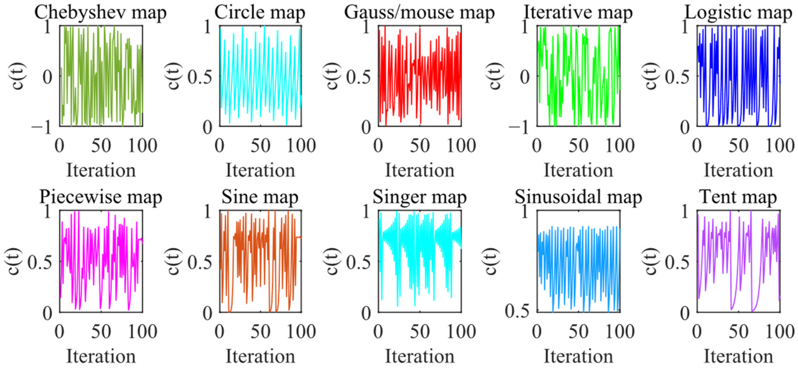
Figure 1. Two-area interconnected power system.
Energies 16 01364 g001
Figure 2. DFIG structure control block diagram.
Energies 16 01364 g002
Figure 3. Cascade 3DOF-FOPID-FOPI controller structure block diagram.
Energies 16 01364 g003
Figure 4. Chaotic mapping image curve.
Energies 16 01364 g004
Figure 5. Flow chart of algorithm optimization.
Energies 16 01364 g005
Figure 6. Dynamic performance under Area 1 2% load disturbance (a) Δ f 1 , (b) Δ f 2 , and (c) Δ P t i e .
Energies 16 01364 g006
Figure 7. Dynamic performance at 2% load disturbance in area 1 and 4% load disturbance in area 2 (a) Δ f 1 , (b) Δ f 2 , and (c) Δ P t i e .
Energies 16 01364 g007
Figure 8. The variation of (a) random wind speed V W , (b) wind turbine output power Δ P W .
Energies 16 01364 g008
Figure 9. Dynamic performance of the system under random wind speed fluctuations. (a) Δ f 1 , (b) Δ f 2 , and (c) Δ P t i e .
Energies 16 01364 g009
Figure 10. Algorithm iteration curve and dynamic system response (a) iterative process of different algorithms, (b) Δ f 1 , (c) Δ f 2 , and (d) Δ P t i e .
Energies 16 01364 g010
Figure 11. Comparison of robustness results under different load disturbances and system parameters (a) Δ f 1 with change in loading condition, (b) Δ f 1 with change in B , (c) Δ f 1 with change in R , (d) Δ f 1 with change in T w , (e) Δ f 1 with change in T 12 , and (f) Δ f 1 with change in T P .
Energies 16 01364 g011
Table 1. The chaotic maps function.
No.Chaotic MapFunctionRange
1Chebyshev y t + 1 = cos ( k cos 1 ( y t ) ) [−1, 1]
2Circle y t + 1 = mod ( ( y t + g ( e / 2 π ) sin ( 2 π y t ) ) , 1 ) e = 0.5 , g = 0.2 [0, 1]
3Gauss/Mouse y t + 1 = 1 y t = 0 1 mod ( y t , 1 ) o t h e r w i s e [0, 1]
4Iterative y t + 1 = sin ( e π / y t ) e = 0.7 [−1, 1]
5Logistic y t + 1 = e y t ( 1 y t ) e = 4 [0, 1]
6Piecewise y t + 1 = y t K   0 y t K y t K 0.5 K   0 y t K 1 K y t 0.5 K 0 y t K 1 y t K 0 y t K   K = 0.4 [0, 1]
7Sine y t + 1 = e 4 sin ( π y t ) e = 4 [0, 1]
8Singer y t + 1 = τ ( 7.86 y t 23.31 y t 2 + 28.75 y t 3 13.302875 y t 4 ) τ = 1.07 [0, 1]
9Sinusoidal y t + 1 = e y t 2 sin ( π y t ) e = 2.3 [0, 1]
10Tent y k + 1 = y t 0.7 y t < 0.7 10 3 ( 1 y t ) y t 0.7 [0, 1]
Table 2. Gains of each controller parameter.
ControllerUnit K P K I K D η ζ P f D f G f f N K P 1 K I 1 η 1
PIDthermal202
hydro202
diesel222
FOPIDthermal22200.9036
hydro0.16771.8687200
diesel22200
2DOF-FOPIDthermal1.91122200.29200.04022.9999
hydro0.9487000.00370.52650.33640
diesel2220.08450.338233
3DOF-FOPIDthermal1.999922012.99103146.5761
hydro1.24941.98580.113310.59322.22412.99770.9536188.0323
diesel2220.0857032.99981143.5195
CC-FOCthermal2020.99130.9186330.083664.6058220.0386
hydro20.064600.88790.999402.9930108.32720.334400.6158
diesel1.99941.99921.99960.159202.99722.99751104.8120220
Table 3. Overshoot/Undershoot and Settling time of state variables for 2% load disturbance in area 1.
Controller Δ f 1 Δ f 2 Δ P t i e ITSE × 10 6
U S × 10 3   ( Hz ) O S × 10 3   ( Hz ) T s   ( sec ) U S × 10 3   ( Hz ) O S × 10 3   ( Hz ) T s   ( sec ) U S × 10 3   ( Hz ) O S × 10 3   ( Hz ) T s   ( sec )
PID−1.410.310.78−0.260.113.2−0.250.13210.52.88
FOPID−1.880.08378.66−0.240.00785.46−0.20.0056.210.79
2DOF-FOPID−0.910.02865.45−0.0740.0014.65−0.0805.650.122
3DOF-FOPID−0.490.03475.35−0.07230.00264.25−0.07450.002234.450.098
CC-FOC−0.14520.00961.276−0.02300.00081.976−0.02090.00061.5760.0078
Table 4. Frequency deviation and tie-line power deviation under sensitivity analysis.
Controller% Change Δ f 1 Δ f 2 Δ P t i e ITSE × 10 6
U S × 10 3 (Hz) O S × 10 3 (Hz) T s (sec) U S × 10 3 (Hz) O S × 10 3 (Hz) T s (sec) U S × 10 3 (Hz) O S × 10 3 (Hz) T s (sec)
Nominal0−0.14520.00961.276−0.02300.00081.976−0.02090.00061.5760.0077
Loading condition+25−0.18160.01191.327−0.02900.00092.505−0.02610.00082.2550.0122
−25−0.10890.00711.142−0.00170.00061.192−0.01560.00051.1420.0044
B = 0.5390+25−0.13270.00871.255−0.01920.00061.505−0.01940.00061.4550.0066
B = 0.3234−25−0.16100.01051.254−0.02860.00102.339−0.02260.00711.7890.0094
R = 3+25−0.14390.00941.279−0.02270.00781.929−0.02070.00641.5290.0077
R = 1.8000−25−0.14660.00961.277−0.02360.00812.027−0.02100.00651.6270.0079
T w = 1.25+25−0.14530.00951.277−0.02320.00791.977−0.02090.00651.5770.0078
T w = 0.75−25−0.14530.00951.278−0.02320.00781.978−0.02080.00651.5780.0078
T 12 = 0.0541+25−0.14460.00871.177−0.02660.00932.133−0.02390.00761.8130.0074
T 12 = 0.0325−25−0.14590.01001.326−0.01920.00611.476−0.01730.00491.5270.0083
T P = 14.3625+25−0.13840.09661.285−0.02330.00802.025−0.02330.08041.6280.0084
T P = 8.6175−25−0.15400.09471.243−0.02300.00781.925−0.02070.00651.5340.0076
Disclaimer/Publisher’s Note: The statements, opinions and data contained in all publications are solely those of the individual author(s) and contributor(s) and not of MDPI and/or the editor(s). MDPI and/or the editor(s) disclaim responsibility for any injury to people or property resulting from any ideas, methods, instructions or products referred to in the content.

