Article

An Enhancement Method Based on Long Short-Term Memory Neural Network for Short-Term Natural Gas Consumption Forecasting

1
College of Petroleum Engineering, Southwest Petroleum University, Chengdu 610500, China
2
Cyberspace Institute of Advanced Technology, Guangzhou University, Guangzhou 510000, China
3
College of Petroleum Engineering, Xi’an Shiyou University, Xi’an 710065, China
4
International Education, University of Exeter, Exeter EX4 4PY, UK
5
Faculty of Engineering & Applied Science, University of Regina, Regina, SK S4S 0A2, Canada
*
Authors to whom correspondence should be addressed.
Energies 2023, 16(3), 1295; https://doi.org/10.3390/en16031295
Submission received: 21 December 2022 / Revised: 19 January 2023 / Accepted: 23 January 2023 / Published: 26 January 2023

Abstract

:
Artificial intelligence models have been widely applied for natural gas consumption forecasting over the past decades, especially for short-term consumption forecasting. This paper proposes a three-layer neural network forecasting model that can extract key information from input factors and improve the weight optimization mechanism of long short-term memory (LSTM) neural network to effectively forecast short-term consumption. In the proposed model, a convolutional neural network (CNN) layer is adopted to extract the features among various factors affecting natural gas consumption and improve computing efficiency. The LSTM layer is able to learn and save the long-distance state through the gating mechanism and overcomes the defects of gradient disappearance and explosion in the recurrent neural network. To solve the problem of encoding input sequences as fixed-length vectors, the layer of attention (ATT) is used to optimize the assignment of weights and highlight the key sequences. Apart from the comparisons with other popular forecasting models, the performance and robustness of the proposed model are validated on datasets with different fluctuations and complexities. Compared with traditional two-layer models (CNN-LSTM and LSTM-ATT), the mean absolute range normalized errors (MARNE) of the proposed model in Athens and Spata are improved by more than 16% and 11%, respectively. In comparison with single LSTM, back propagation neural network, support vector regression, and multiple linear regression methods, the improvement in MARNE exceeds 42% in Athens. The coefficient of determination is improved by more than 25%, even in the high-complexity dataset, Spata.

1. Introduction

As a high-energy intensity and low-carbon energy source, natural gas plays a vital role in achieving “Carbon Peaking and Carbon Neutrality” targets [1]. Global natural gas consumption has continued to rise and annually increased by 2.9% in the past 10 years. In 2021, natural gas consumption accounted for 24.7% of primary energy consumption [2]. Natural gas consumption forecasting, especially for daily short-term forecasting, is crucial for pipeline optimization, gas distribution, and economic feasibility analysis of natural gas pipeline systems [3]. As the contract between dispatchers and users is generally on a daily basis, the dispatch management, planning, and operation optimization of the gas pipeline system rely on accurate daily consumption forecasting [4]. An accurate and automatic daily forecasting system is also an important part of intelligent pipeline network systems, which is being implemented in many cities. Therefore, the accuracy of daily gas consumption forecasting methods is of great significance in improving the management and economics of gas supply systems and ensuring a safe and uninterrupted gas supply [5].
Since Verhulst et al. [6] developed the first demand forecasting model for French gas demand in 1950, various short-term consumption forecasting models were further proposed. These models can be generally divided into conventional statistical methods and artificial intelligence (AI)-based methods. The conventional methods include multiple linear regression (MLR) [7], gray model [8], autoregressive moving average model [9], etc. Artificial intelligence methods include support vector machines [10] and artificial neural networks (ANNs). With the improvement in computer processing capabilities, artificial intelligence forecasting models based on machine learning overcome the defect of conventional statistical methods that are difficult to learn complex patterns from nonlinear time series data [11] and construct multiple improved neural networks and support vector regression (SVR) models. Compared with traditional neural networks, recurrent neural networks (RNNs) enhance the ability to save historical information [12]. As a special branch of RNN, the long short-term memory (LSTM) neural network is considered the most popular time series forecasting method in various fields, which solves the problem of gradient disappearance and explosion during the long-distance transmission of RNN [13].
Muzaffar and Afshari [14] utilized LSTM to forecast daily consumption for the following seven and thirty days. The results indicated that the LSTM model outperformed conventional statistical models and achieved the lowest mean absolute percentage error (5.97% and 9.75%). Kong et al. [15] proved that the performance of LSTM was better than that of conventional neural network models for forecasting the short-term consumption of a single residential home. Peng et al. [16] proposed a novel combined forecasting model integrating local mean decomposition, wavelet threshold denoising, and LSTM approaches to forecast daily consumption in London. Compared with single methods, the proposed combined model presented an excellent performance in short-term natural gas consumption forecasting.
However, recent studies have found that the LSTM model has two inherent shortcomings: (1) it cannot extract key features from input factors [17], and (2) it also cannot overcome the defect of encoding input sequences as a fixed-length hidden vector [18].
In order to draw major components from the input factors, feature selection and feature extraction methods are used to eliminate the redundant components of the time series features and improve the computing efficiency of LSTM [19]. Wei et al. [20] suggested an enhanced principal component analysis method and integrated it with LSTM to forecast daily consumption in Xi’an, China, and Athens, Greece. The proposed method extracted key information from input factors, and also eliminated redundant components and minimized the data dimension. Wu et al. [21] constructed a novel feature extraction method that improved the accuracy of LSTM by 49% and was at least 17% superior to other forecasting methods. In terms of feature selection methods, the elastic-net regularized generalized linear model, spike-slab lasso method, and Bayesian model average method were compared to select the appropriate features for the input of the LSTM neural network by Lu et al. [22]. The results implied that the accuracy of the short-term consumption forecasting model was apparently enhanced by the combination with the feature selection method. Although feature selection methods for optimizing the input of the LSTM model reduce the feature dimension by examining the relationship between features, the filter strategy may eliminate the critical information that has a great impact on time series forecasting results [17]. Additionally, feature extraction approaches only evaluate the spatial characteristics between features, the temporal characteristics between samples, which are crucial for time series forecasting, are not discussed [23].
Furthermore, to improve the second shortcoming of the LSTM model, multiple variants of the LSTM model, such as bidirectional LSTM, stacked LSTM, etc., were developed to optimize the model structure. Shahid et al. [18] utilized bidirectional LSTM, which consists of forward and backward LSTM neural networks, to forecast the confirmed cases of COVID-19. The outputs of forward and backward hidden vectors at each moment were concatenated to represent a fuller hidden layer output. The experimental results indicated that bidirectional LSTM enhanced the structure of hidden vectors and exhibited better performance. Sebt et al. applied stacked LSTM that comprised multiple LSTM layers to forecast the number of customer transactions [24] and concluded that the performance of their proposed stacked LSTM model was superior to recurrent neural network, prophet, and Autoregressive Integrated Moving Average model (ARIMA) models. However, the proposal of bidirectional LSTM and stacked LSTM cannot overcome the defect that the typical encoding-decoding LSTM model encodes the input sequences into fixed-length hidden vectors while learning and saving the long-distance state [25]. As the length of the input sequence increases, each hidden vector is still assigned the same weight, and the LSTM model cannot distinguish the importance among hidden vectors [26]. Some crucial spatial and temporal information will be ignored during the training process and resulting in worse performance. Thus, a mechanism is required to assist the LSTM model in evaluating the significance of hidden vectors at different moments in the input sequence and highlighting the key factors in the hidden vectors.
Motivated by the above analysis, the aim of this paper is to provide an effective feature extraction method that can extract temporal and spatial characteristics for the input of LSTM and solve the problem that the hidden vectors of LSTM share the same weight. The proposed method suggests a novel LSTM optimization framework, which comprises the convolutional neural network, LSTM, and attention mechanism. The convolutional neural network is used to extract the major components of the input sequence from the perspectives of spatial and temporal characteristics and reconstruct a new feature pattern for LSTM input. Then, the LSTM neural network is applied to forecast time series data. The attention mechanism is set behind LSTM to evaluate the significance of hidden vectors at different moments in the input sequence. It can adaptively draw hidden vectors from the LSTM layer and assign varying attention to hidden vectors at different moments so as to highlight the major components. Additionally, to evaluate the robustness and accuracy of the proposed model, we design two real-life scenarios with different fluctuation characteristics and analyze the effect on various types of datasets.

2. Methodology

This section describes the algorithm and framework of the combination model used in this paper. The proposed three-layer neural network forecasting model consists of three approaches: convolutional neural network (CNN) algorithm for improving the input of LSTM, LSTM benchmark algorithm, and attention mechanism (ATT) for optimizing the weight distribution of hidden vectors. The strategy and framework of the proposed CNN-LSTM-ATT model are presented in Section 2.4.

2.1. Convolutional Neural Network

The convolutional neural network (CNN) is a deep learning-based neural network that is typically used to analyze data with a known grid topology in fields such as time series analysis, computer vision, and natural language processing. The structure of the CNN consists of an input layer, a convolutional layer (kernel and convolutional output), a pooling layer, and an output layer [27]. A schematic of the convolutional neural network is depicted in Figure 1.
It can be seen from Figure 1 that the convolutional layer is the major component of CNN; it extracts spatial and temporal characteristics from the input features based on the predefined convolutional kernel and uses an activation function to perform a nonlinear transformation on each convolutional result to map the initially linearly indistinguishable multidimensional features to another space.
The pooling layer is set behind the convolutional layer. The feature map calculated from the convolutional layer is scanned in a step-by-step manner. Then, the maximum value within the filter is captured in turn to reduce the number of connections between neurons in the convolutional layer and perform secondary feature extraction on the input features.
CNN can automatically learn spatial and temporal features from the input data and has the advantages of local connection, weight sharing, pooling operation, and multi-layer structure, which simplify the complexity of LSTM input. The gradient descent optimization approach applied in CNN reduces overfitting and provides better generalizability. For certain sequences, the effect of one-dimensional convolution can be compared with recurrent neural networks and only requires less computing cost [28]. The equations for the convolutional layer and pooling layer are as follows:
Convolutional layer:
x j l = f i M j x i l 1 k i j l + b j l
Pooling layer:
P i l + 1 j = max j 1 w + 1 t j w q i l t
where x i l 1 and x i l represent the output of layer (l − 1) and layer l, respectively; k i j l is the convolution kernel of layer l; b, Mj, and w represent the bias, input feature vector, and width of the pooling area, respectively; q i l t is the value of the tth neuron in the ith feature vector of layer l; and P i l + 1 j is the value corresponding to the neuron of layer (l + 1).

2.2. Long Short-Term Memory

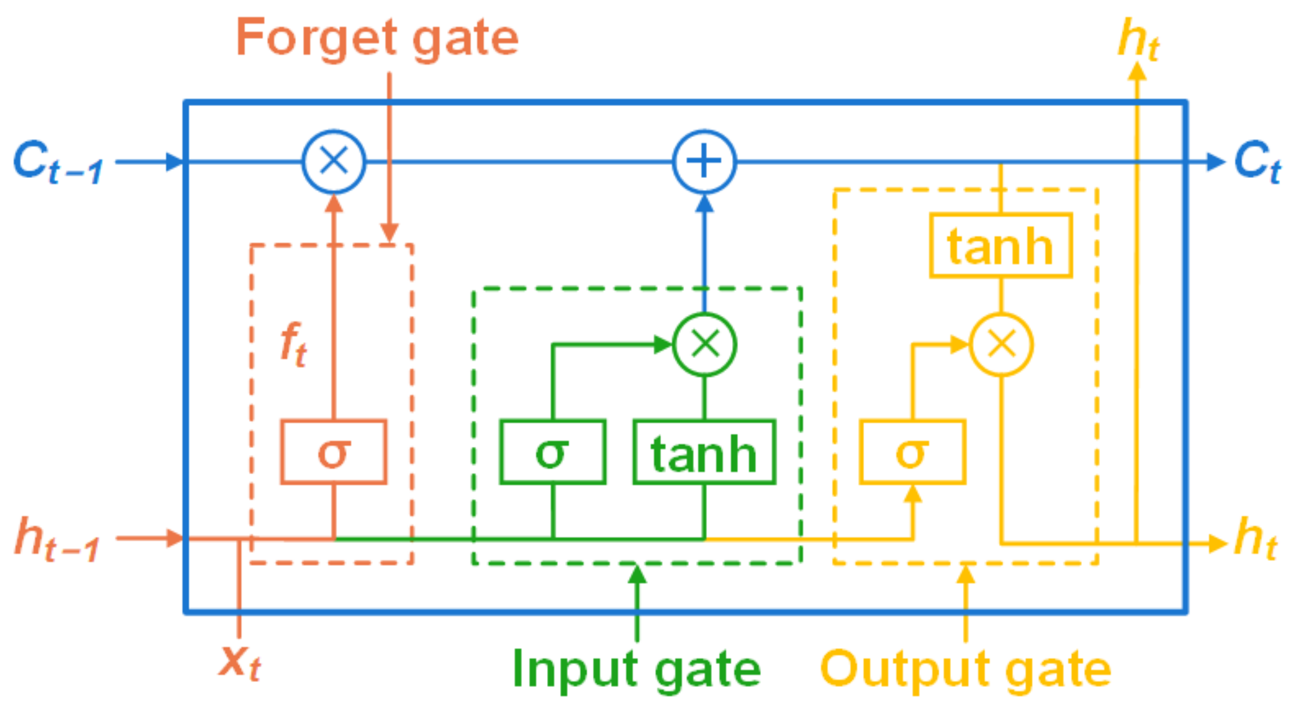
The long short-term memory (LSTM) algorithm was proposed by Hochreiter [29] in 1997. The principle is to continuously update the weights through a gating mechanism to learn and save long-term memory of time series data. It avoids the problems of gradient disappearance and explosion in RNNs and serves as the most popular forecasting model in time series forecasting. The cell structure of LSTM is shown in Figure 2. The equations of LSTM can be described as follows:
(1)
Forget gate: the forget gate reflects the ability to learn historical information.
f t = σ W f h t 1 , x t + b f
(2)
Input gate: the input gate performs the selectivity of the memory module by utilizing a nonlinear function to determine which portion of the input information will be stored.
i t = σ W i h t 1 , x t + b i
C ˜ t = tanh W C h t 1 , x t + b C
Update cell status:
C t = f t C t 1 + i t C ˜ t
(3)
Output gate: the function of the output gate is to update the parameters of hidden layers, including selective learning and preservation of historical data. The new cell state and hidden vector state will be transmitted to the subsequent time step.
o t = σ W o h t 1 , x t + b o
h t = o t tanh C t
where Ct, C ˜ t , and Ct-1 represent cell status; xt and ht are the vector states at time t; and W and b are the weights and biases, respectively.

2.3. Attention Mechanism

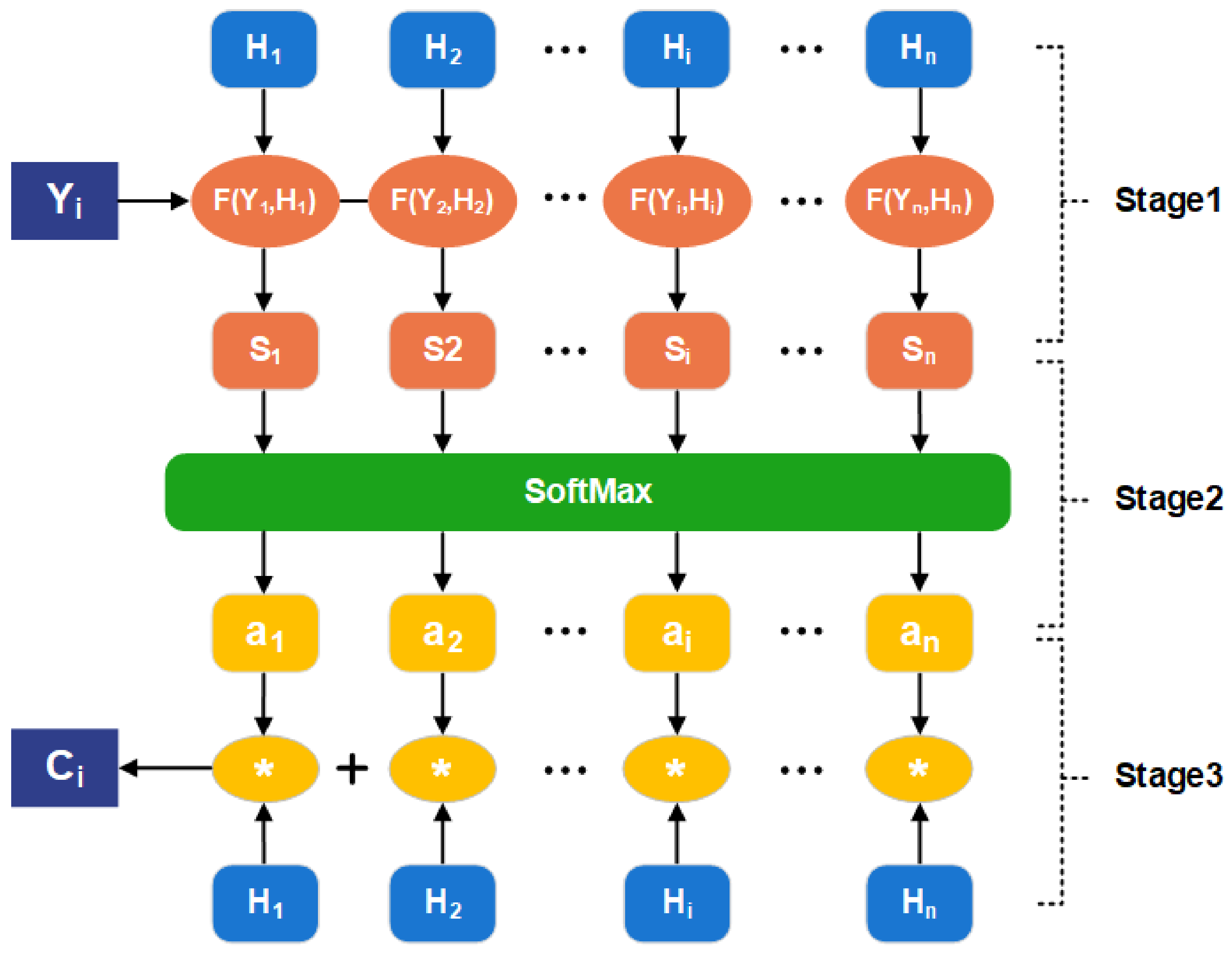
Attention mechanism is derived from the principle of human visual focus, which simulates the characteristics of human beings unconsciously focusing on the key positions in a picture [30]. Given this, attention mechanism is designed to concentrate the limited computing ability on key information in the collected data so that it can save computing costs and process information efficiently. Its essence is to learn an appropriate weight distribution for input features so that the model focuses on high-weight features and pays less attention to low-weight features [31]. Figure 3 presents the structure of the attention mechanism.
The process of the attention mechanism can be separated into three stages. The first stage is to calculate the similarity Si between Yi and each Hi. In the second stage, softmax normalization is performed on the similarity scores, and the attention value is calculated by the weighted sum of Hi and weight coefficient. The equations can be expressed as follows:
S i = tanh W H i + b i
α i = s o f t max S i
C i = i = 1 k α i H i
where Hi is the output of the LSTM hidden layer; Si represents the similarity score; W and α i are the weight matrix and weight coefficient, respectively; and Ci represents the attention value.

2.4. Strategy of the Proposed Model

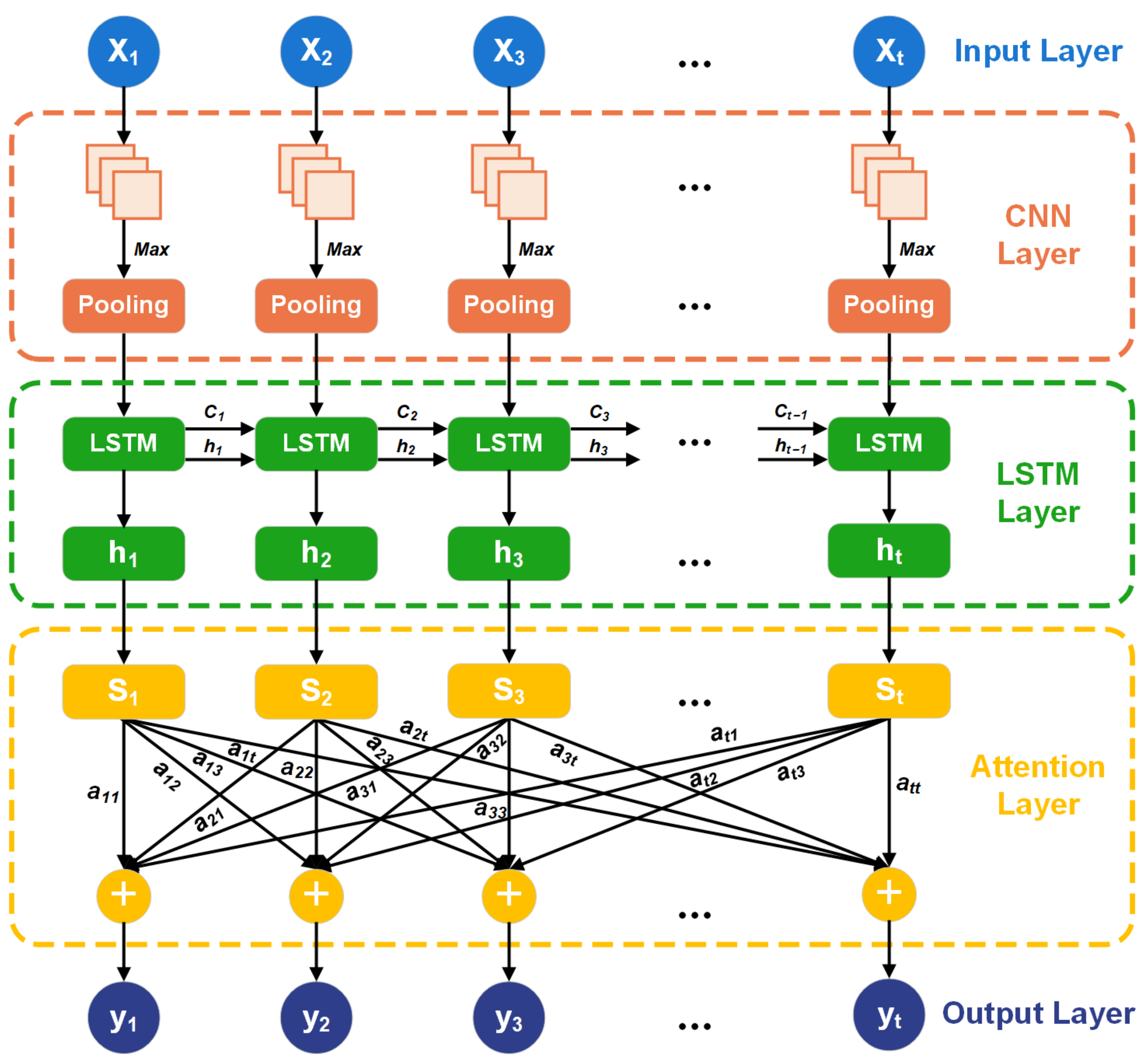
Figure 4 describes the strategy of the proposed enhancement method for LSTM. The first step is to add a CNN layer to optimize the input of LSTM. The convolution operation in CNN adaptively extracts spatial and temporal features from the sample data and transmits them into the LSTM model as the optimized input. Then, the LSMT layer is used to learn and save the long-distance state of input through the gating mechanism.
To solve the problem that the LSTM model assigns the same weight to the hidden vector h, the third layer is designed as the attention layer. During the decoding process, the attention mechanism is used to evaluate the importance of different hidden vectors h and assign appropriate weights to them. That is, we can learn the weight distribution of hidden vectors in LSTM and pay more attention to high-weight features so that it can improve forecasting performance and efficiency. Furthermore, the model limitations are discussed to complete our research.

3. Results and Discussion

The purpose of the experiments is to reveal the enhancement effect of the convolutional neural network and attention mechanism on LSTM and validate the model performance and robustness in terms of accuracy. Based on this, our experiments can be divided into two parts. The first part validates the performance of the proposed model compared to LSTM, which combined only one enhancement method, attention or CNN. Part two evaluates the performance of the proposed model and four popular forecasting models, including single LSTM, back-propagation neural network (BPNN), SVR, and MLR, and validates the model robustness on two datasets with different complexities.

3.1. Evaluation Methods

Evaluation indicators used in regression forecasting algorithms include MARNE (mean absolute range normalized error), MAPE (mean absolute percentage error), R2 (coefficient of determination), MSE (mean squared error), MAE (mean absolute error), and RMSE (root-mean-square error). To validate the model robustness on the two designed datasets, MSE, MAE, and RMSE affected by the order of magnitude are not suitable for evaluating the forecasting results. Thus, MARNE, MAPE, and R2 are utilized as the major evaluation indicators in our research.
MARNE:
M A R N E = 100 % n × i = 1 n y ˜ i y i max ( y ˜ i )
MAPE:
M A P E = 100 % n × i = 1 n y ˜ i y i y i
R2:
R 2 = 1 i = 1 n y ˜ i y i 2 i = 1 n y ¯ i y i 2
where y ˜ i ,  y i , and y ¯ i represent the forecast data, actual data, and average of data y, respectively; and n is the number of samples.

3.2. Data Description

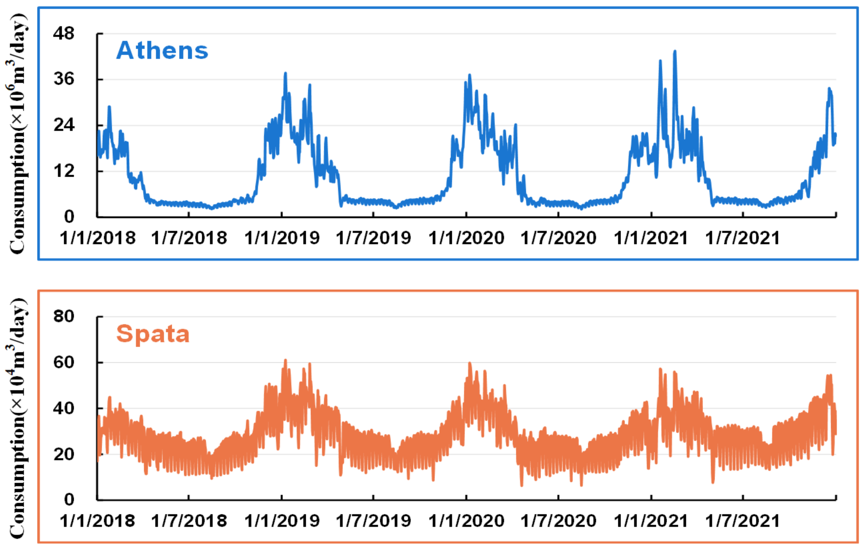
To evaluate the robustness and performance of the proposed CNN-LSTM-ATT model, it is validated on two datasets with different complexities and fluctuations. The designed datasets are collected from two nodes in the Greek gas pipeline network, ranging from 1 January 2018 to 31 December 2021. The consumption curves are shown in Figure 5.
The complexity of consumption is determined by the sample entropy, which is specially researched to describe the complexity index of time series data [32]. High sample entropy means high complexity, indicating that the fluctuation of time series data is more complex. It is a widely used index for measuring complexity [33]. Table 1 shows the sample entropy, training, and testing data size of the designed datasets.
It can be seen from Figure 5 that Athens has an obvious seasonal periodic trend. The fluctuation is mainly concentrated from December to March of the next year and is more complicated in 2021, which is the forecasting target of this paper. The fluctuation of Spata is apparently more complicated than that of Athens. It presents a weak seasonal periodicity trend, and the fluctuations between data points are more concentrated. The sample entropies calculated in Table 1 also prove that Spata (2.10) has nearly twice the complexity of Athens. Thus, it can be found that Athens and Spata are time series datasets with different complexities from the perspectives of consumption curve and sample entropy, which can be perfectly applied to validate the robustness of the proposed model.
Influencing factors affecting the fluctuation of natural gas consumption can be selected as input factors for model training. Wei et al. [34] collected 19 weather profiles from the weather company of IBM for daily consumption forecasting. Sabo et al. [35] analyzed the implicit, explicit, functional, and linear dependence of natural gas consumption on temperature and demonstrated that natural gas consumption and temperature are explicitly related. According to the natural gas consumption forecasting review report conducted by Soldo [36], Tamba et al. [37], and Liu et al. [38], short-term gas consumption is significantly affected by weather profiles and temperature. Thus, factors related to temperature and weather profiles are regarded as the input data for model training to improve the nonlinear fitting ability. In this work, we focus on daily natural gas consumption; therefore, all data we mentioned will be daily data without any specifications.

3.3. Experimental Setup

Considering that the length of time series data is 1096, the LSTM benchmark forecasting model used in this paper is set to a single LSTM layer. Maximum pooling as a method of secondary extraction in the convolutional layer is not appropriate for regression forecasting with a limited data size. Two feature extractions may change the original fluctuations, making the model learn incorrect patterns and reducing the forecasting accuracy. Thus, the feature extraction layer is set to a single CNN layer. The attention layer is set behind the LSTM layer to reassign different weights to the hidden vectors of LSTM. The number of neurons in CNN and LSTM layers, as well as the batch size and epochs, are determined by the GridsearchCV function [39], CV = 5. Other parameters used in the models are determined by trial and error.
Furthermore, all methods mentioned in this paper are coded in Python 3.8. The neural network functions and structures are constructed based on the package Keras 2.4.3, which was developed by Google.

3.4. Factor Selection

The factors of the two profiles (temperature and weather profiles) related to natural gas consumption include maximum, average, and minimum temperatures; maximum, average, and minimum dew points; maximum, average, and minimum humidities; and maximum, average, and minimum pressures. Those 12 factors are used as the input data of the model for daily forecasting. The Pearson correlation coefficient is used to select the highly correlated factors among the 12 factors. Table 2 shows the Pearson correlation coefficients between consumption and temperature and weather profiles.
It can be seen from Table 2 that features from temperature and dew point profiles present a higher correlation to natural gas consumption and indicate a negative correlation. Among those 12 factors, the maximum and average temperatures and maximum dew point have the higher absolute correlation coefficients and are selected as the input factors of the forecasting models in this paper.

3.5. Performance Discussion

To evaluate the improvement obtained from the convolutional neural network and attention mechanism on LSTM in terms of accuracy, we first compare the improvement from the single and combined enhancement methods to LSTM. Then, it is compared with other popular forecasting models to prove the robustness of the proposed model.

3.5.1. Comparison between Two Enhanced Methods for LSTM

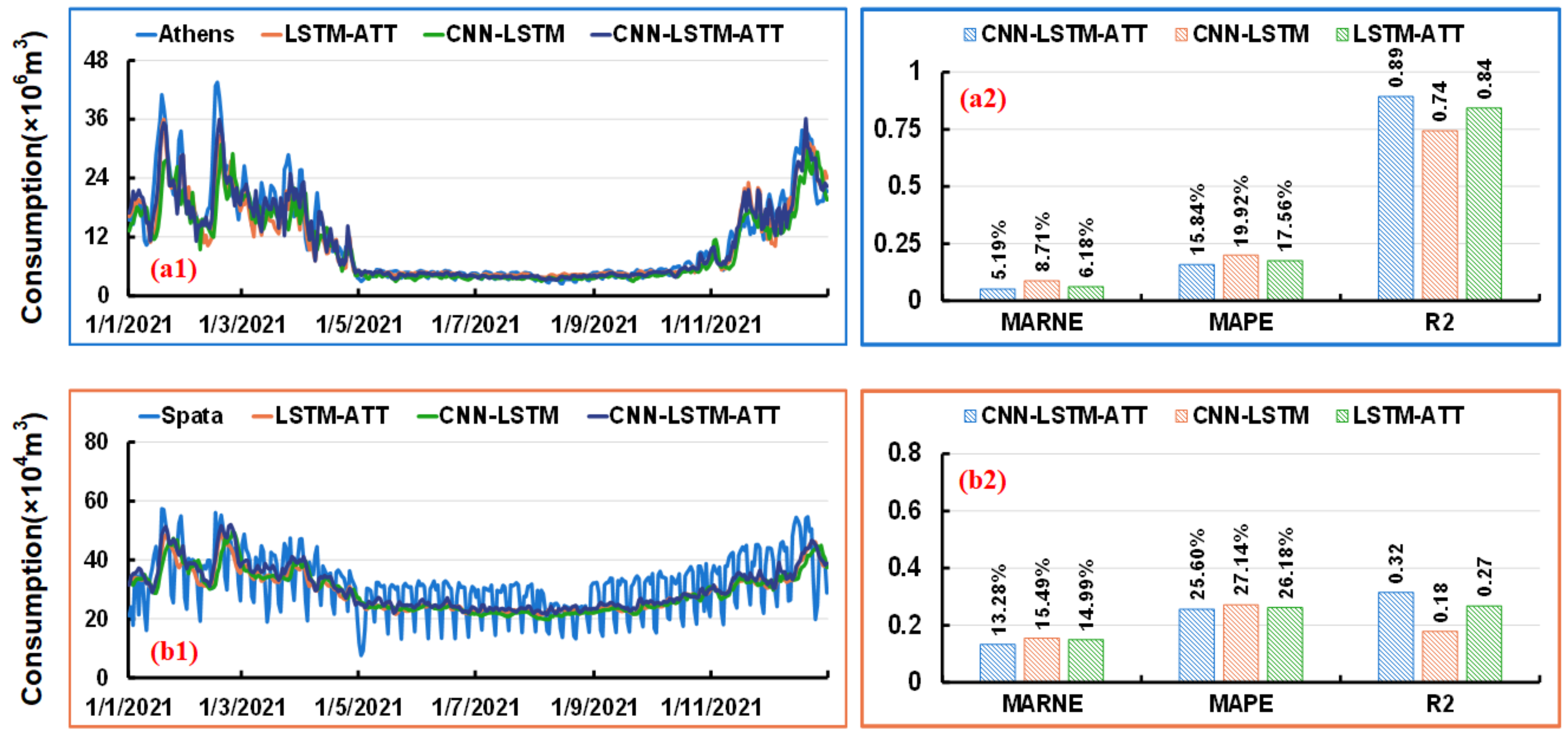
As two enhancement methods of LSTM, CNN-LSTM and LSTM-ATT, are utilized to compare with the proposed model to find the best forecasting method appropriate for datasets with different complexities. Figure 6 and Table 3 show the forecasting curves, errors, and computational cost (seconds per series) [40] of the three enhancement methods for LSTM.
Figure 6 shows that the forecasting curve of our proposed model perfectly fits the peak and trough of the real consumption curve Figure 6(a1). Although the forecasting results of Spata with high sample entropy are not as accurate as Athens, the proposed algorithm is closest to the actual curve compared with other enhancement methods Figure 6(b1). It can also be found from Figure 6(a2,b2) that CNN-LSTM-ATT has the highest R2 and lowest MARNE and MAPE in Athens and Spata.
All indicators in Table 3 indicate that CNN-LSTM-ATT outperforms CNN-LSTM and LSTM-ATT in the designed datasets. Compared with CNN-LSTM, the evaluation indicators of the proposed model are improved by more than 20% in Athens and by more than 5% in Spata. The MARNE, MAPE, and R2 are improved by 16.03%, 9.80%, and 5.93%, respectively, in Athens as against LSTM-ATT. In Spata, the indicators are improved by 11.38%, 2.21%, and 17.54%, respectively. Additionally, it is apparent that the computational cost is shorter than CNN-LSTM and LSTM-ATT. The improvement implies that our proposed LSTM enhancement method presents superiority over other combined methods on datasets with different complexities. Although the improvement of the attention mechanism to LSTM is better than CNN, only the combination of the three methods can take full advantage of each method. Additionally, the proposed model should be compared with other popular forecasting models to validate the model’s performance.

3.5.2. Comparison with Other Forecasting Models

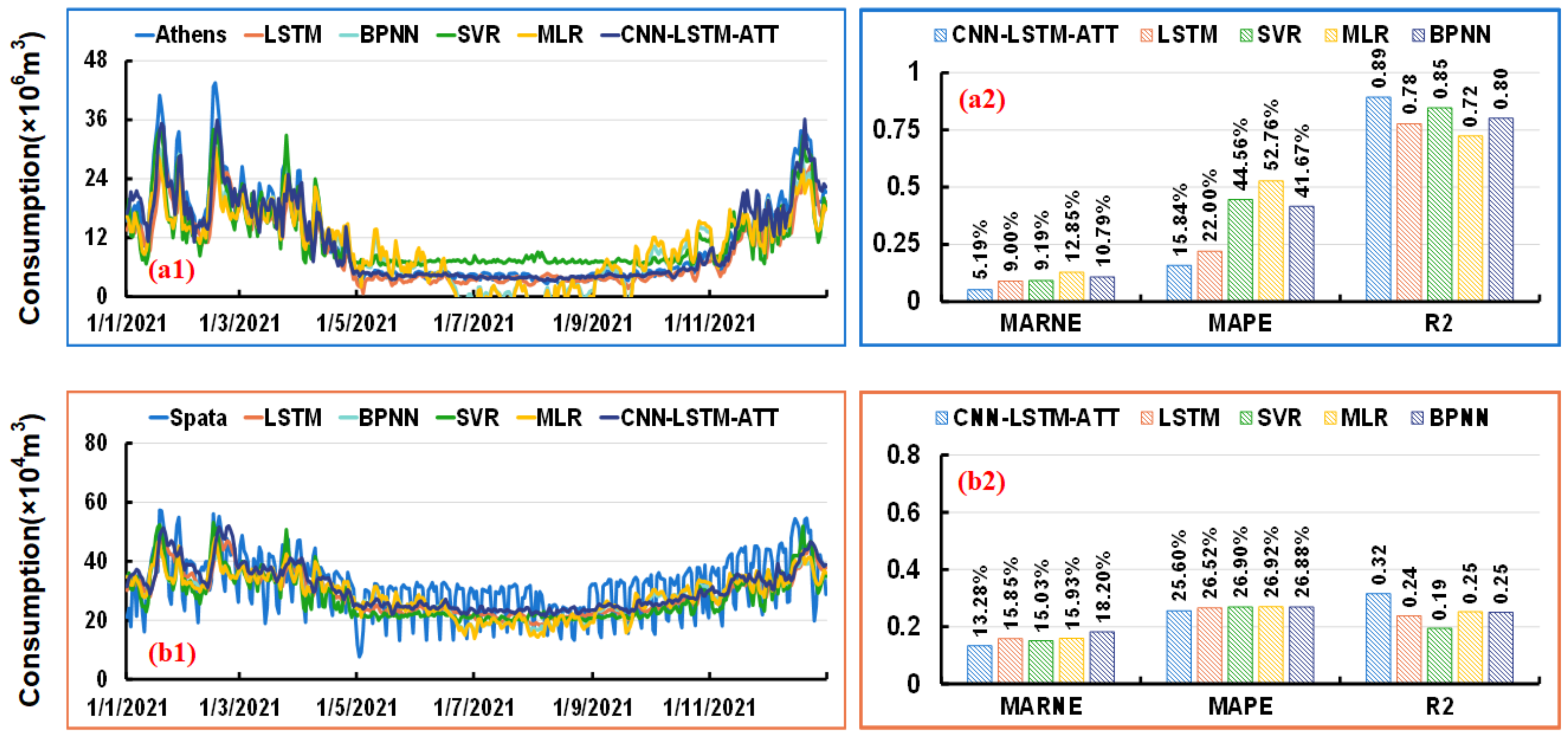
The above analysis proves that the proposed model is superior to other LSTM enhancement methods. However, it is still necessary to compare the proposed model with other popular forecasting models to evaluate the model performance and robustness on datasets with different complexities. Figure 7 and Table 4 present the forecasting curves, errors, and computational cost (seconds per series) [41] between CNN-LSTM-ATT and other forecasting models.
It can be seen from Figure 7 that the forecasting results of LSTM and BPNN are closer to the real consumption curve than SVR and MLR, which deviate far from the original curve, but it is clear that CNN-LSTM-ATT perfectly describes the real consumption curve. Figure 7(b1) presents that the forecasting results of the other four methods deviate from the original consumption curve for dataset Spata with higher complexity. Although the proposed method cannot fit the original curve well either, it obtains better results. The indicators in Figure 7(a2,b2) also prove that CNN-LSTM-ATT presents the best forecasting performance.
Table 4 indicates that the MARNE, MAPE, and R2 of the proposed model are improved by more than 42%, 27%, and 5%, respectively, in Athens compared with LSTM, SVR, and MLR. In Spata, the proposed model improves R2 by more than 25%. The improvement in MARNE is 16.23%, 11.61%, and 16.61%, respectively. The MAPE is improved by 3.47%, 4.83%, and 4.93%, respectively. All indicators imply that the proposed model shows the best robustness and performance. Additionally, the computational cost of classic statistical methods MLR and SVR is shorter than ANN methods BPNN, LSTM, and CNN-LSTM-ATT. This is because ANN methods take extra time to fit complex nonlinear relationships through model training. It is obvious that our proposed method takes less training time than BPNN and LSTM.
From the above analysis, it can be concluded that the superiority of the CNN-LSTM-ATT model has been validated on datasets with different complexities. The proposed method demonstrates better performance and robustness than other popular forecasting models and can be applied to datasets with different complexities in various real-life scenarios.

4. Conclusions

This paper proposes a novel three-layer neural network forecasting model, namely, CNN-LSTM-ATT, which consists of a CNN layer, an LSTM layer, and the attention mechanism. The CNN layer extracts major components, including spatial and temporal information, from the input factors. The LSTM layer is used to learn and save the long-distance state of time series data. The attention mechanism adaptively redistributes the weight of the LSTM hidden vectors to overcome the defect of encoding input sequences into fixed-length vectors. Two datasets with different sample entropies and fluctuation characteristics are designed to evaluate the model’s robustness. Given this, the most important findings are as follows:
I
Compared with two enhancement methods for LSTM, the combined approach of CNN, LSTM, and attention mechanism takes full advantage of each algorithm and achieves better performance. Compared with CNN-LSTM, the evaluation indicators of the proposed model are improved by more than 20% in Athens and by more than 5% in Spata. The MARNE of the proposed model is improved by more than 11% in the two designed datasets as against LSTM-ATT.
II
The proposed enhancement method for LSTM significantly improves forecasting accuracy. Compared with single LSTM, SVR, and MLR, CNN-LSTM-ATT perfectly fits the peak and trough of the consumption curves and exhibits the best performance and robustness. The results indicate that the improvement of the proposed model on MARNE, MAPE, and R2 exceeds 42%, 27%, and 5% in Athens, respectively. The R2 is improved by more than 25%, even in the high-complexity dataset, Spata.
In this paper, the proposed three-layer neural network forecasting model proves its superiority in terms of model performance and robustness and can be regarded as a reliable forecasting method to provide consumption distribution plans for natural gas pipeline companies. However, we also found that the limitation of the model lies in the structure and parameters of the neural network. The optimal structure and parameters used in this paper are tested via trial and error, and a lot of time is spent throughout the experiments. Additionally, model performance is affected by the correlation between input factors and natural gas consumption. The low correlation input factors result in weak performance. To further improve the model performance and efficiency, the feature enhancement method will be considered to improve the correlation, and mathematical methods will be considered to find the optimal network structure and parameters in the future.

Author Contributions

Conceptualization, J.L.; methodology, J.L.; writing—original draft preparation, J.L.; funding acquisition, S.W. and N.W.; investigation, Y.Y. and Y.L.; data curation, X.W.; supervision, F.Z. and X.W.; writing—review and editing, F.Z. All authors have read and agreed to the published version of the manuscript.

Funding

This research was funded by the China Scholarship Council, grant number 202109225009; the Guangdong Basic and Applied Basic Research Foundation, grant number 2021A1515012454; the Guangzhou Basic Research Program-City School (College) Joint Funding Project, grant number 202201010609; the Young Talent Support Project of Guangzhou Association for Science and Technology, grant number QT20220101122; and the Research Project of Guangzhou University, grant number RP2021012.

Institutional Review Board Statement

Not applicable.

Informed Consent Statement

Not applicable.

Data Availability Statement

The datasets generated and supporting the findings of this article are obtainable from the corresponding author upon reasonable request.

Conflicts of Interest

The authors declare no conflict of interest.

References

  1. Liu, C.; Wu, W.-Z.; Xie, W.; Zhang, T.; Zhang, J. Forecasting natural gas consumption of China by using a novel fractional grey model with time power term. Energy Rep. 2021, 7, 788–797. [Google Scholar] [CrossRef]
  2. BP plc. BP Statistical Review of World Energy 2021; BP: London, UK, 2021. [Google Scholar]
  3. Deng, C.; Zhang, X.; Huang, Y.; Bao, Y. Equipping seasonal exponential smoothing models with particle swarm optimization algorithm for electricity consumption forecasting. Energies 2021, 14, 4036. [Google Scholar] [CrossRef]
  4. Wei, N.; Li, C.; Li, C.; Xie, H.; Du, Z.; Zhang, Q.; Zeng, F. Short-term forecasting of natural gas consumption using factor selection algorithm and optimized support vector regression. J. Energy Resour. Technol. 2019, 141, 032701. [Google Scholar] [CrossRef]
  5. Beyca, O.F.; Ervural, B.C.; Tatoglu, E.; Ozuyar, P.G.; Zaim, S. Using machine learning tools for forecasting natural gas consumption in the province of Istanbul. Energy Econ. 2019, 80, 937–949. [Google Scholar] [CrossRef]
  6. Verhulst, M.J. The theory of demand applied to the French gas industry. Econom. J. Econom. Soc. 1950, 18, 45–55. [Google Scholar] [CrossRef]
  7. Gil, S.; Deferrari, J. Generalized model of prediction of natural gas consumption. J. Energy Resour. Technol. 2004, 126, 90–98. [Google Scholar] [CrossRef]
  8. Fan, G.; Wang, A.; Hong, W. Combining grey model and self-adapting intelligent grey model with genetic algorithm and annual share changes in natural gas demand forecasting. Energies 2018, 11, 1625. [Google Scholar] [CrossRef] [Green Version]
  9. Akpinar, M.; Yumusak, N. Forecasting household natural gas consumption with ARIMA model: A case study of removing cycle. In Proceedings of the International Conference on Application of Information and Communication Technologies, Washington, DC, USA, 12–14 October 2022; pp. 1–6. [Google Scholar]
  10. Bai, Y.; Sun, Z.; Zeng, B.; Long, J.; Li, L.; de Oliveira, J.V.; Li, C. A comparison of dimension reduction techniques for support vector machine modeling of multi-parameter manufacturing quality prediction. J. Intell. Manuf. 2019, 30, 2245–2256. [Google Scholar] [CrossRef]
  11. Lu, H.; Azimi, M.; Iseley, T. Short-term load forecasting of urban gas using a hybrid model based on improved fruit fly optimization algorithm and support vector machine. Energy Rep. 2019, 5, 666–677. [Google Scholar] [CrossRef]
  12. Hribar, R.; Potocnik, P.; Silc, J.; Papa, G. A comparison of models for forecasting the residential natural gas demand of an urban area. Energy 2019, 167, 511–522. [Google Scholar] [CrossRef]
  13. Wei, N.; Yin, L.; Li, C.; Wang, W.; Qiao, W.; Li, C.; Zeng, F.; Fu, L. Short-term load forecasting using detrend singular spectrum fluctuation analysis. Energy 2022, 256, 124722. [Google Scholar] [CrossRef]
  14. Muzaffar, S.; Afshari, A. Short-term load forecasts using LSTM networks. Energy Procedia 2019, 158, 2922–2927. [Google Scholar] [CrossRef]
  15. Kong, W.; Dong, Z.Y.; Jia, Y.; Hill, D.J.; Xu, Y.; Zhang, Y. Short-term residential load forecasting based on LSTM recurrent neural network. IEEE Trans. Smart Grid 2017, 10, 841–851. [Google Scholar] [CrossRef]
  16. Peng, S.; Chen, R.; Yu, B.; Xiang, M.; Lin, X.; Liu, E. Daily natural gas load forecasting based on the combination of long short term memory, local mean decomposition, and wavelet threshold denoising algorithm. J. Nat. Gas Sci. Eng. 2021, 95, 104175. [Google Scholar] [CrossRef]
  17. Hira, Z.M.; Gillies, D.F. A review of feature selection and feature extraction methods applied on microarray data. Adv. Bioinform. 2015, 2015, 198363. [Google Scholar] [CrossRef]
  18. Shahid, F.; Zameer, A.; Muneeb, M. Predictions for COVID-19 with deep learning models of LSTM, GRU and Bi-LSTM. Chaos Solitons Fractals 2020, 140, 110212. [Google Scholar] [CrossRef]
  19. Qiao, W.; Yang, Z.; Kang, Z.; Pan, Z. Short-term natural gas consumption prediction based on volterra adaptive filter and improved whale optimization algorithm. Eng. Appl. Artif. Intell. 2020, 87, 103323. [Google Scholar] [CrossRef]
  20. Wei, N.; Li, C.; Duan, J.; Liu, J.; Zeng, F. Daily natural gas load forecasting based on a hybrid deep learning model. Energies 2019, 12, 218. [Google Scholar] [CrossRef] [Green Version]
  21. Wu, Y.X.; Wu, Q.B.; Zhu, J.Q. Data-driven wind speed forecasting using deep feature extraction and LSTM. IET Renew. Power Gener. 2019, 13, 2062–2069. [Google Scholar] [CrossRef]
  22. Lu, Q.; Sun, S.; Duan, H.; Wang, S. Analysis and forecasting of crude oil price based on the variable selection-LSTM integrated model. Energy Inform. 2021, 4, 47. [Google Scholar] [CrossRef]
  23. Nakra, A.; Duhan, M. Feature Extraction and Dimensionality Reduction Techniques with Their Advantages and Disadvantages for EEG-Based BCI System: A Review. IUP J. Comput. Sci. 2020, 14, 21–34. [Google Scholar]
  24. Sebt, M.V.; Ghasemi, S.; Mehrkian, S. Predicting the number of customer transactions using stacked LSTM recurrent neural networks. Soc. Netw. Anal. Min. 2021, 11, 86. [Google Scholar] [CrossRef]
  25. Zdravković, M.; Ćirić, I.; Ignjatović, M. Explainable heat demand forecasting for the novel control strategies of district heating systems. Annu. Rev. Control 2022, 53, 405–413. [Google Scholar] [CrossRef]
  26. Yang, T.; Li, B.; Xun, Q. LSTM-attention-embedding model-based day-ahead prediction of photovoltaic power output using Bayesian optimization. IEEE Access 2019, 7, 171471–171484. [Google Scholar] [CrossRef]
  27. Le, T.; Vo, M.T.; Vo, B.; Hwang, E.; Rho, S.; Baik, S.W. Improving electric energy consumption prediction using CNN and Bi-LSTM. Appl. Sci. 2019, 9, 4237. [Google Scholar] [CrossRef] [Green Version]
  28. Kim, T.-Y.; Cho, S.-B. Predicting residential energy consumption using CNN-LSTM neural networks. Energy 2019, 182, 72–81. [Google Scholar] [CrossRef]
  29. Hochreiter, S.; Schmidhuber, J. Long short-term memory. Neural Comput. 1997, 9, 1735–1780. [Google Scholar] [CrossRef]
  30. Bu, S.-J.; Cho, S.-B. Time series forecasting with multi-headed attention-based deep learning for residential energy consumption. Energies 2020, 13, 4722. [Google Scholar] [CrossRef]
  31. Jung, S.; Moon, J.; Park, S.; Hwang, E. An attention-based multilayer GRU model for multistep-ahead short-term load forecasting. Sensors 2021, 21, 1639. [Google Scholar] [CrossRef]
  32. Wei, N.; Yin, L.; Li, C.; Liu, J.; Li, C.; Huang, Y.; Zeng, F. Data complexity of daily natural gas consumption: Measurement and impact on forecasting performance. Energy 2022, 238, 122090. [Google Scholar] [CrossRef]
  33. Montesinos, L.; Castaldo, R.; Pecchia, L. On the use of approximate entropy and sample entropy with centre of pressure time-series. J. Neuroeng. Rehabil. 2018, 15, 116. [Google Scholar] [CrossRef] [PubMed] [Green Version]
  34. Wei, N.; Yin, L.; Li, C.; Li, C.; Chan, C.; Zeng, F. Forecasting the daily natural gas consumption with an accurate white-box model. Energy 2021, 232, 121036. [Google Scholar] [CrossRef]
  35. Sabo, K.; Scitovski, R.; Vazler, I.; Zekić-Sušac, M. Mathematical models of natural gas consumption. Energy Convers. Manag. 2011, 52, 1721–1727. [Google Scholar] [CrossRef]
  36. Soldo, B. Forecasting natural gas consumption. Appl. Energy 2012, 92, 26–37. [Google Scholar] [CrossRef]
  37. Tamba, J.G.; Essiane, S.N.; Sapnken, E.F.; Koffi, F.D.; Nsouandélé, J.L.; Soldo, B.; Njomo, D. Forecasting natural gas: A literature survey. Int. J. Energy Econ. Policy 2018, 8, 216–249. [Google Scholar]
  38. Liu, J.; Wang, S.; Wei, N.; Chen, X.; Xie, H.; Wang, J. Natural gas consumption forecasting: A discussion on forecasting history and future challenges. J. Nat. Gas Sci. Eng. 2021, 90, 103930. [Google Scholar] [CrossRef]
  39. Aljaman, B.; Ahmed, U.; Zahid, U.; Reddy, V.M.; Sarathy, S.M.; Jameel, A.G.A. A comprehensive neural network model for predicting flash point of oxygenated fuels using a functional group approach. Fuel 2022, 317, 123428. [Google Scholar] [CrossRef]
  40. Petropoulos, F.; Grushka-Cockayne, Y. Fast and frugal time series forecasting. arXiv 2021, arXiv:2102.13209. [Google Scholar] [CrossRef]
  41. Hewamalage, H.; Ackermann, K.; Bergmeir, C. Forecast Evaluation for Data Scientists: Common Pitfalls and Best Practices. arXiv 2022, arXiv:2203.10716. [Google Scholar] [CrossRef]
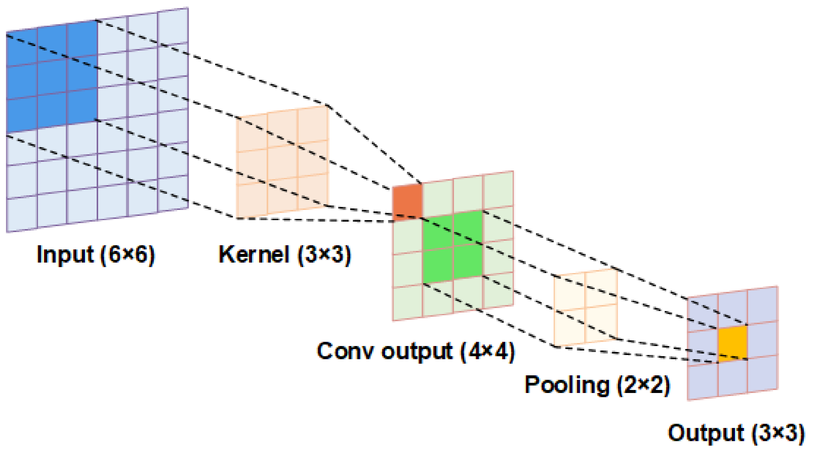
Figure 1. The structure of the convolutional neural network.
Energies 16 01295 g001
Figure 2. The structure of a single LSTM cell.
Energies 16 01295 g002
Figure 3. The structure of the attention mechanism (* represent multiplication).
Energies 16 01295 g003
Figure 4. Framework of the proposed model.
Energies 16 01295 g004
Figure 5. Consumption curves in two datasets with different fluctuation characteristics.
Energies 16 01295 g005
Figure 6. The forecasting curves and errors of two enhanced methods for LSTM.
Energies 16 01295 g006
Figure 7. The forecasting curves and errors between CNN-LSTM-ATT and other forecasting models.
Energies 16 01295 g007
Table 1. Description of the sample entropy and data size.
CitySample EntropyTraining DataTesting Data
Athens1.251 January 2018–31 December 20201 January 2021–31 December 2021
Spata2.101 January 2018–31 December 20201 January 2021–31 December 2021
Table 2. Pearson correlation coefficient between climate profile and consumption.
FactorsAthensSpataFactorsAthensSpata
TemperatureMax−0.86−0.65HumidityMax0.360.30
Avg−0.85−0.64Avg0.460.35
Min−0.78−0.59Min0.470.35
Dew PointMax−0.80−0.60PressureMax0.400.33
Avg−0.78−0.59Avg0.310.26
Min−0.73−0.54Min0.200.18
Table 3. Forecasting results of the three enhanced methods for LSTM.
MethodsAthensSpata
MARNEMAPER2CostMARNEMAPER2Cost
CNN-LSTM-ATT5.19%15.84%0.8940.9613.28%25.60%0.3217.10
CNN-LSTM8.71%19.92%0.7456.7115.49%27.14%0.1830.78
LSTM-ATT6.18%17.56%0.8445.0414.99%26.18%0.2717.61
Table 4. Forecasting results of different models.
MethodsAthensSpata
MARNEMAPER2CostMARNEMAPER2Cost
CNN-LSTM-ATT5.19%15.84%0.8940.9613.28%25.60%0.3217.10
LSTM9.00%22.00%0.7836.5915.85%26.52%0.2427.14
SVR9.19%44.56%0.850.3715.03%26.90%0.190.38
MLR12.85%52.76%0.721.3815.93%26.92%0.250.28
BPNN10.79%41.67%0.8087.1918.20%26.88%0.2587.85
Disclaimer/Publisher’s Note: The statements, opinions and data contained in all publications are solely those of the individual author(s) and contributor(s) and not of MDPI and/or the editor(s). MDPI and/or the editor(s) disclaim responsibility for any injury to people or property resulting from any ideas, methods, instructions or products referred to in the content.