

The Influence of Distributed Generation on the Operation of the Power System, Based on the Example of PV Micro-Installations

 , ,
, ,  , ,
, ,
Abstract
1. Introduction
1.1. Changes in the Root Mean Square and Supply Voltage Frequency
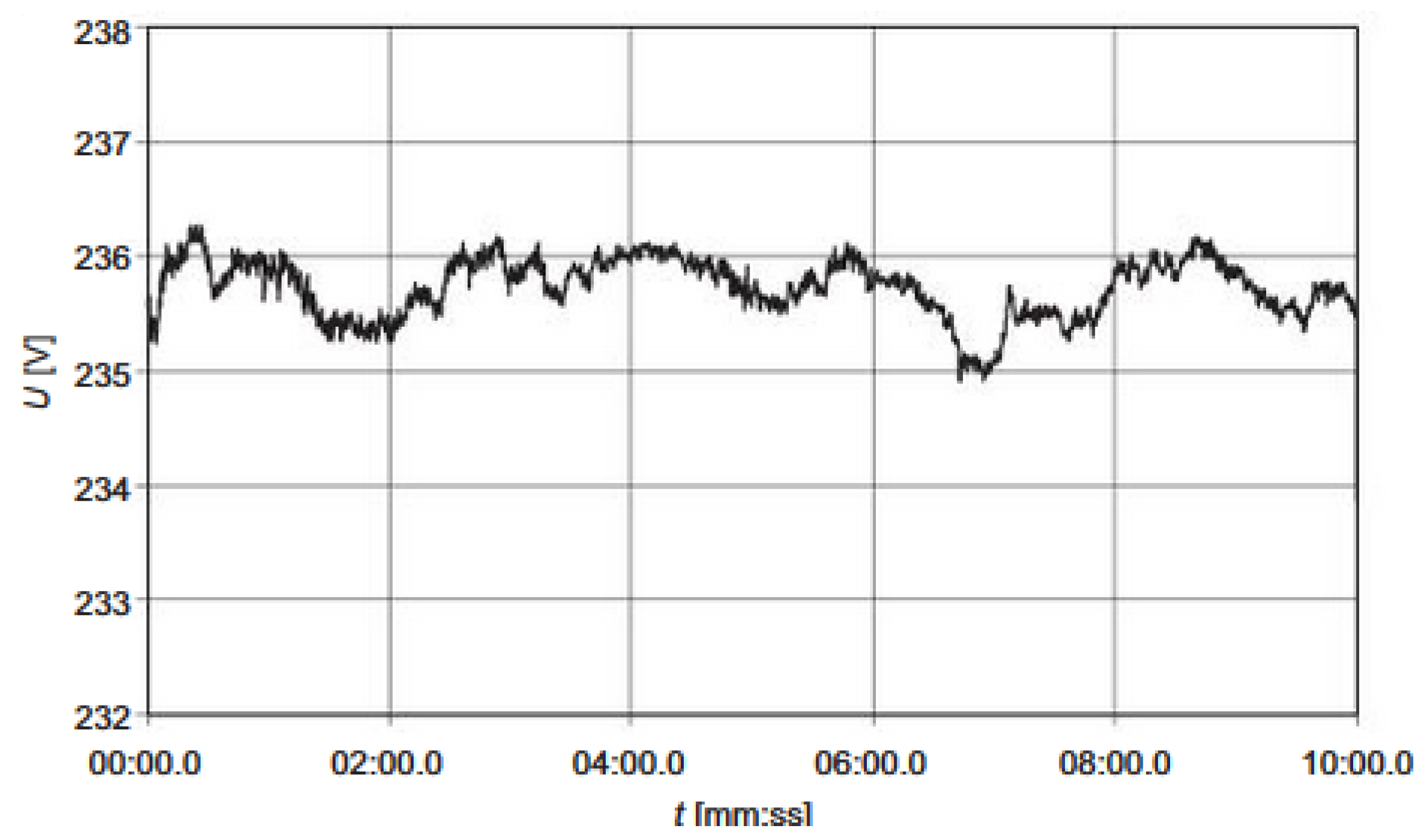
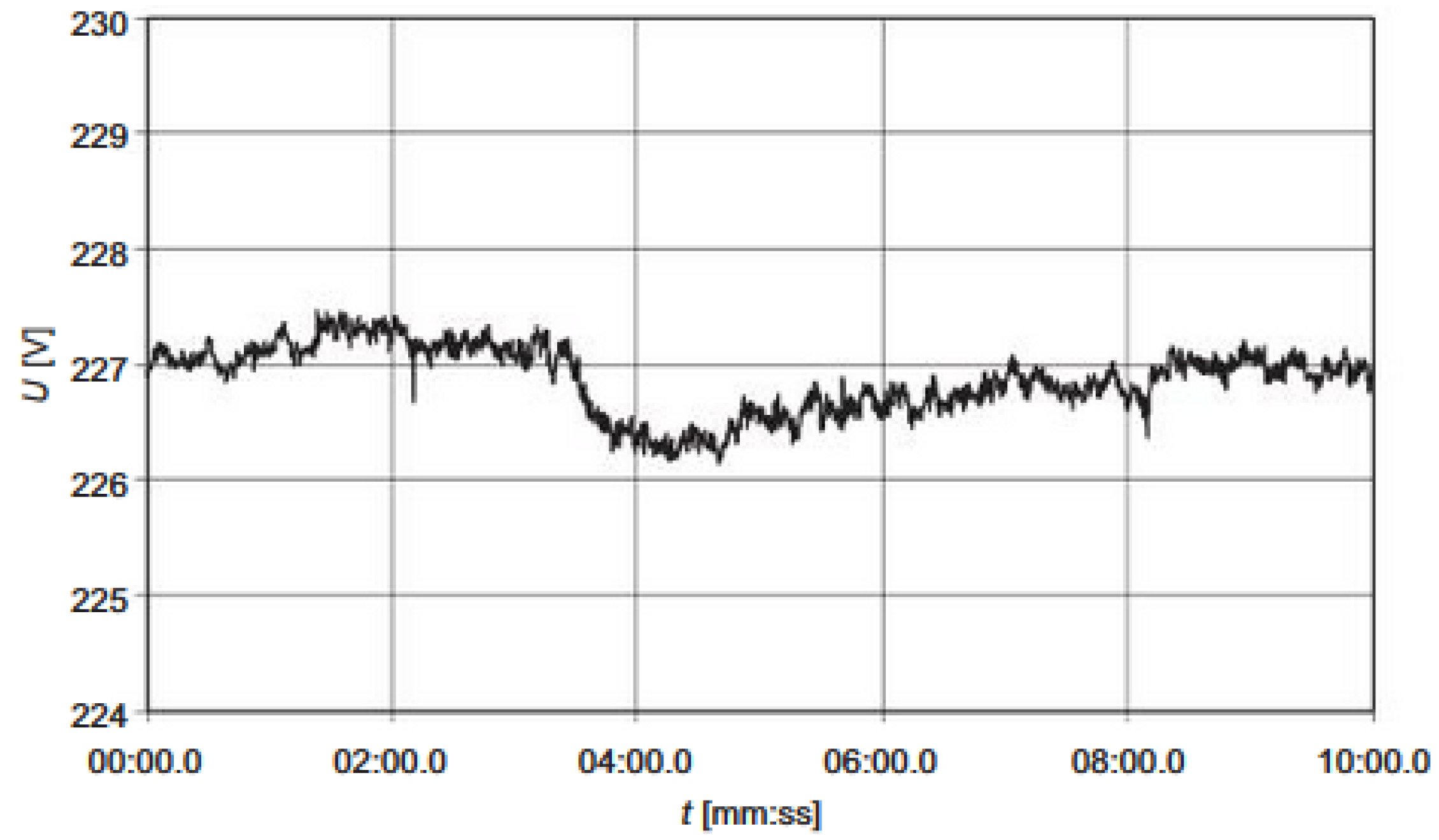
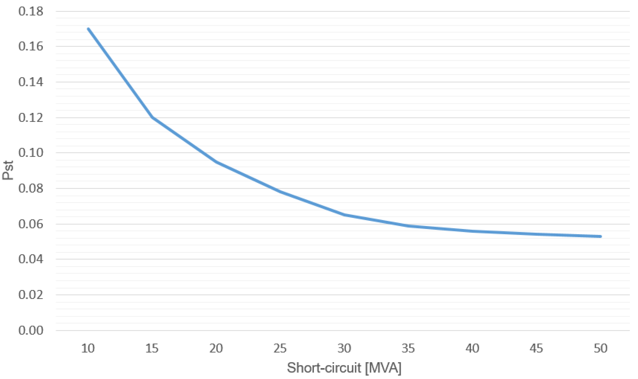
1.2. Voltage Fluctuations
1.3. Voltage Asymmetry
1.4. Voltage and Current Harmonics
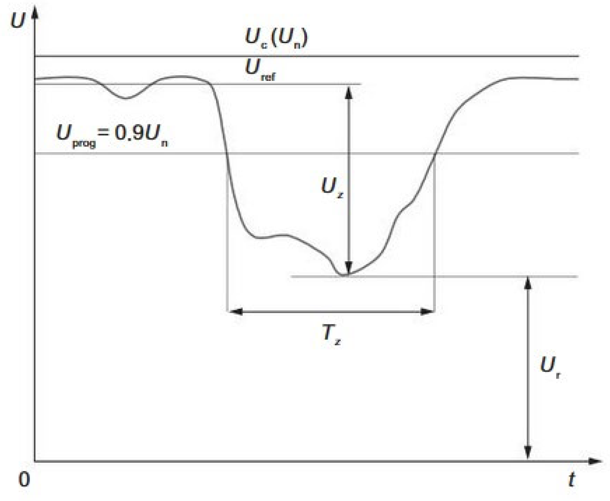
1.5. Voltage Dips
1.6. Behaviour of Consumers That Reduces Voltage Fluctuations
1.7. Overview of Global PV Systems
2. Materials and Methods
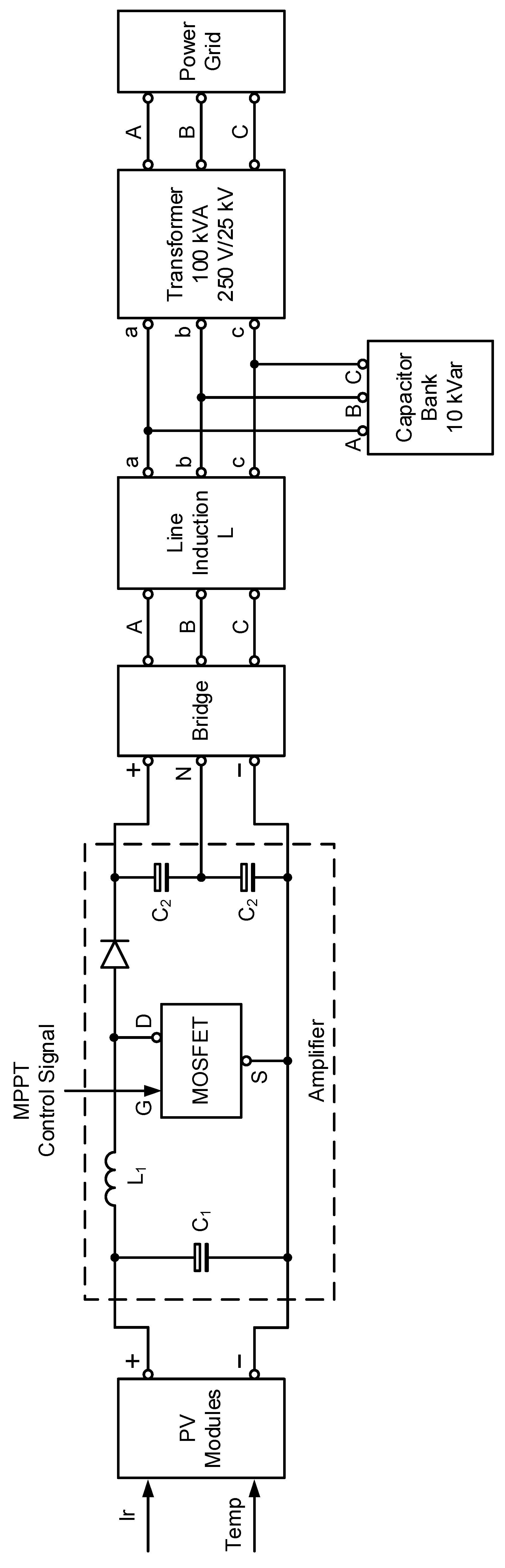
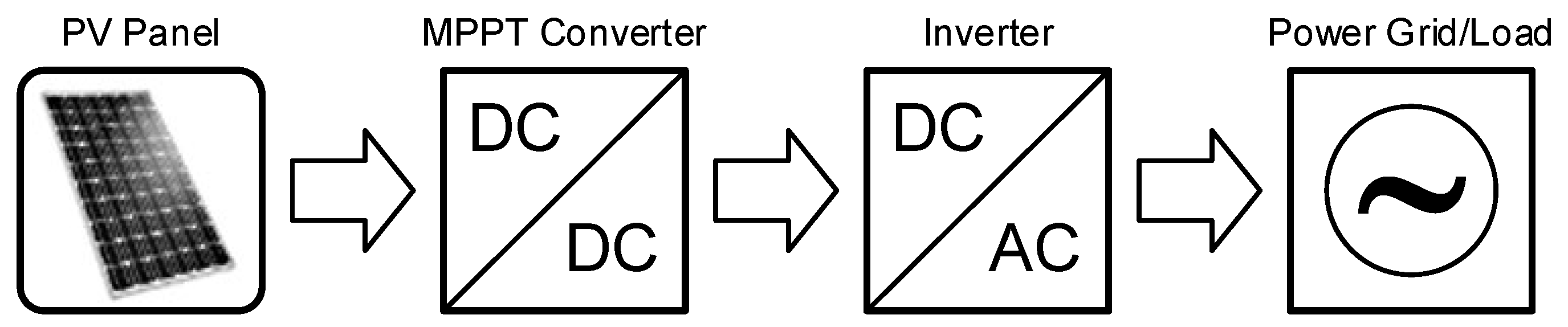
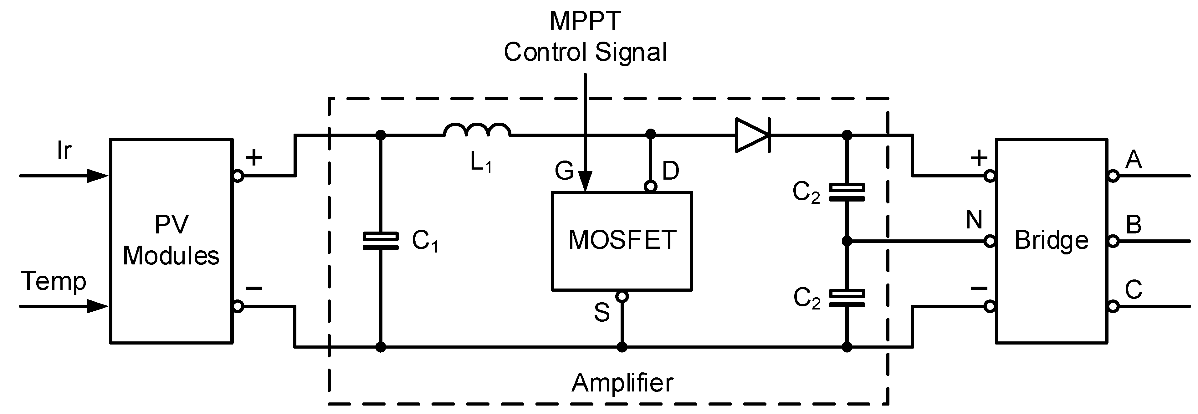
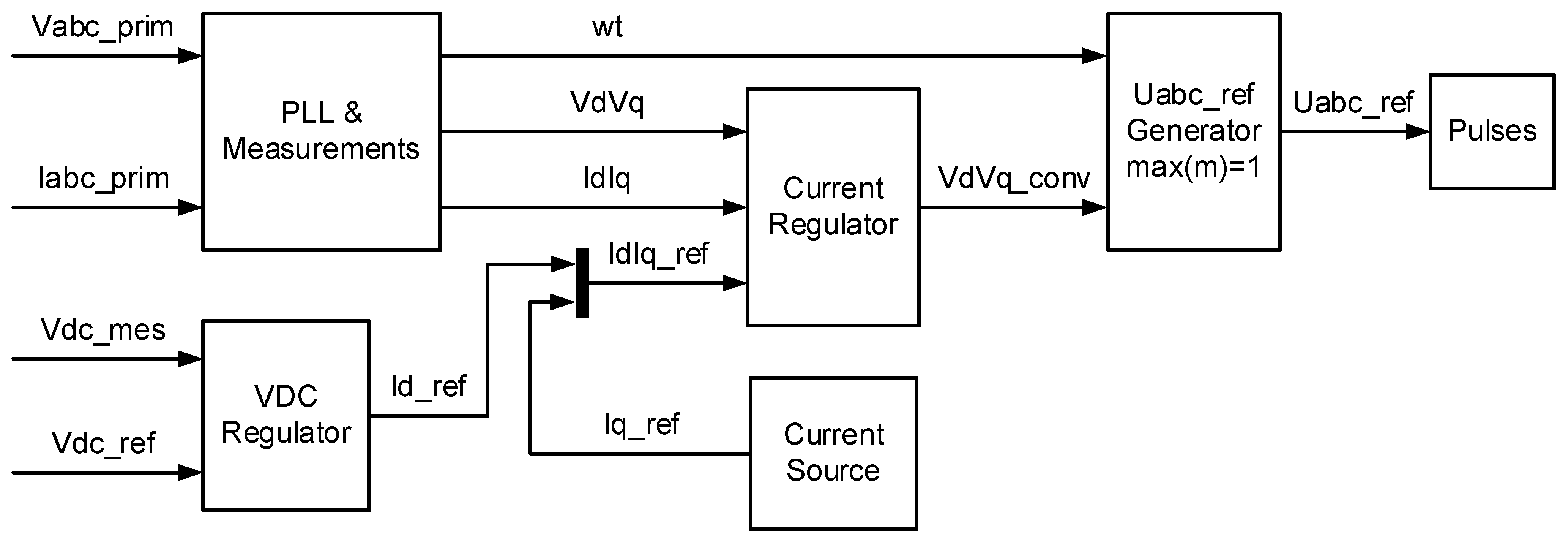
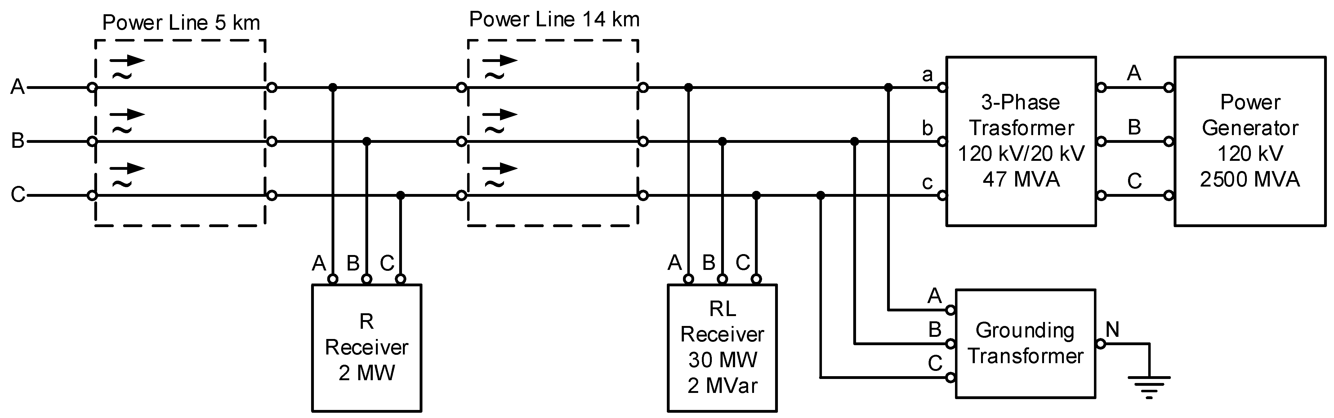
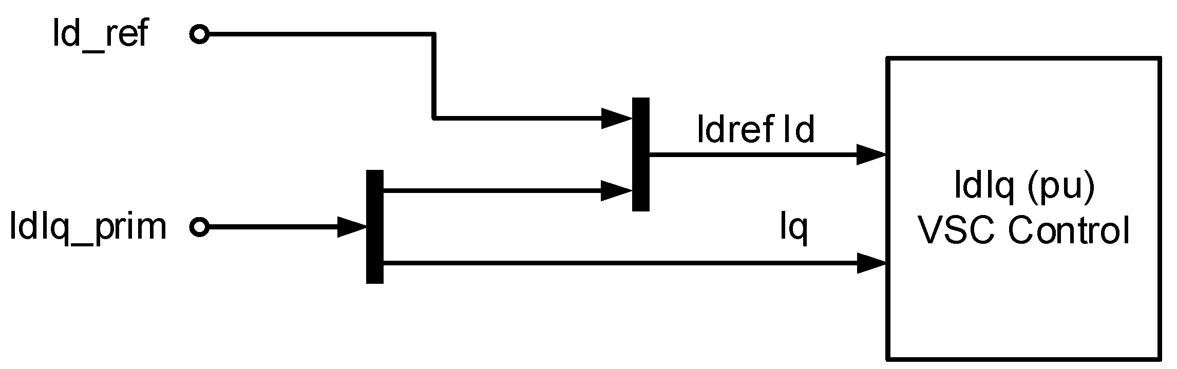
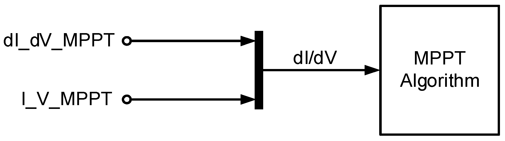
2.1. Description of the Model of the System with the On-Grid Photovoltaic Installation
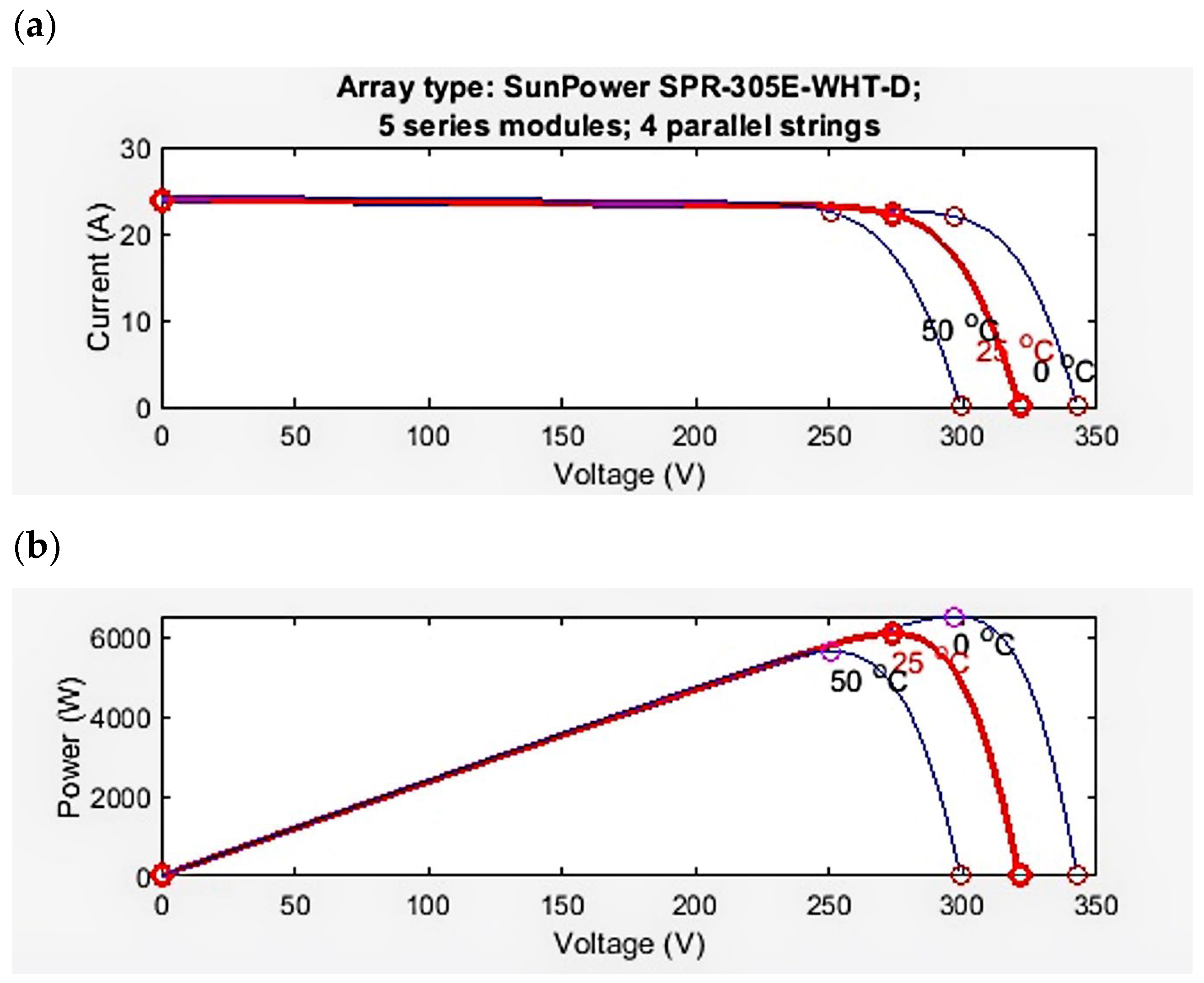
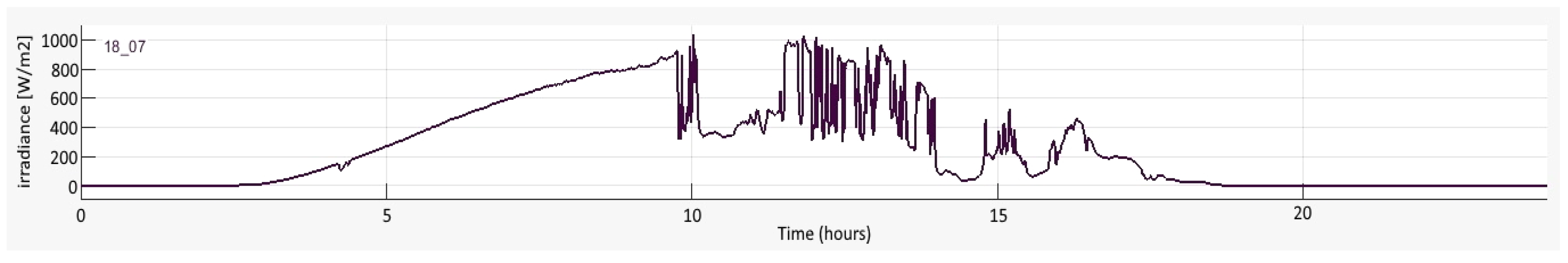
2.2. Input Data for Simulation
3. Results and Discussion—Simulation of the Interaction of the PV Micro-Installation with the Power System
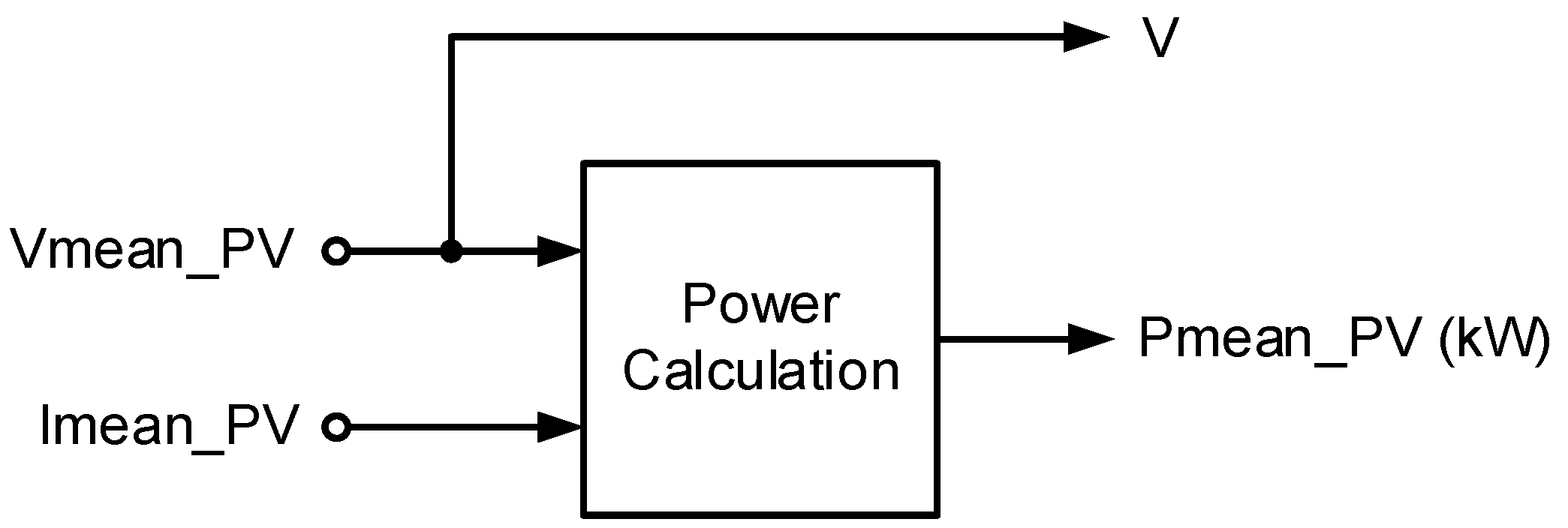
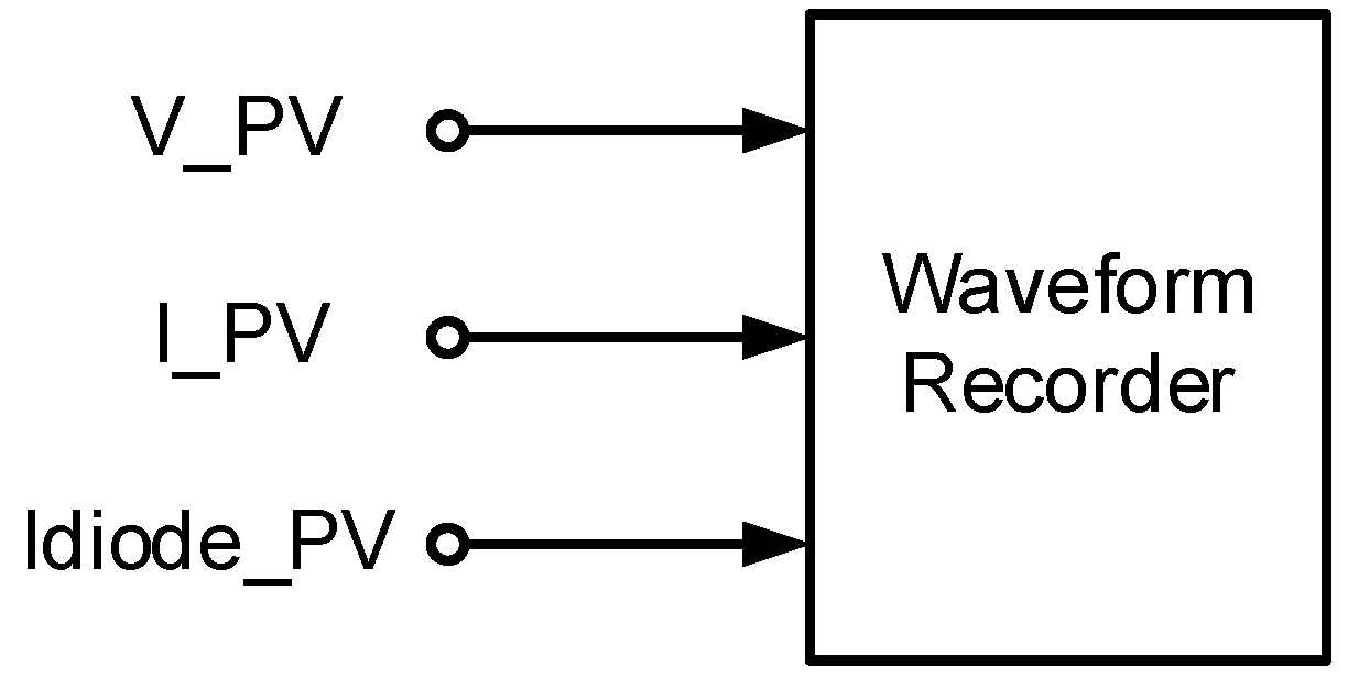
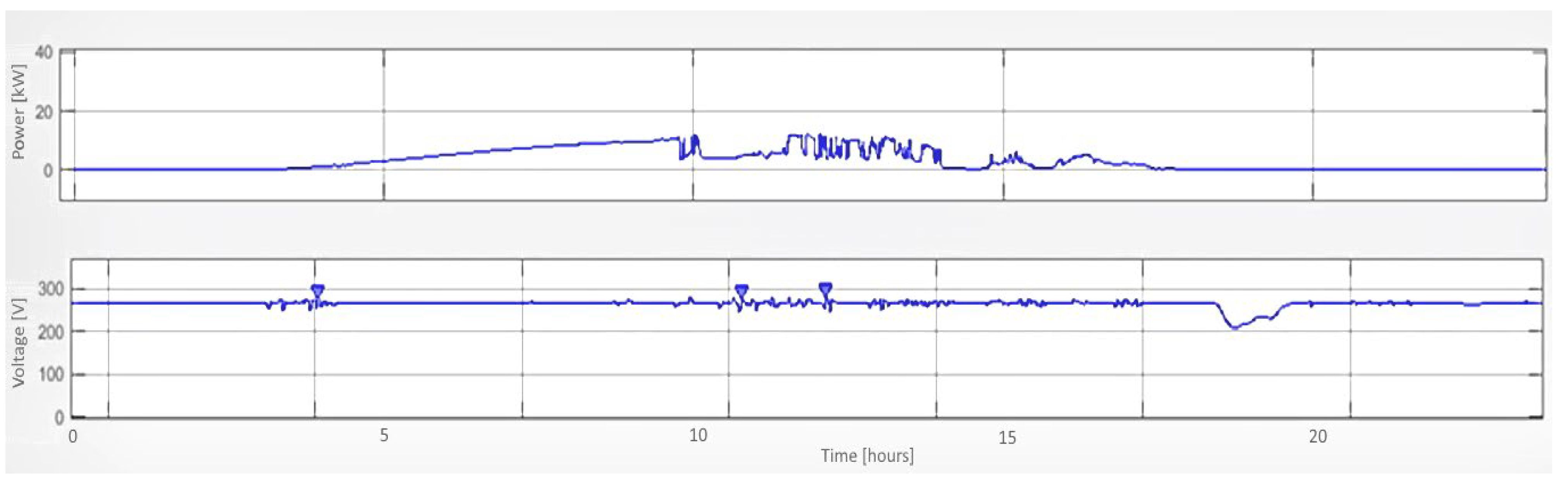
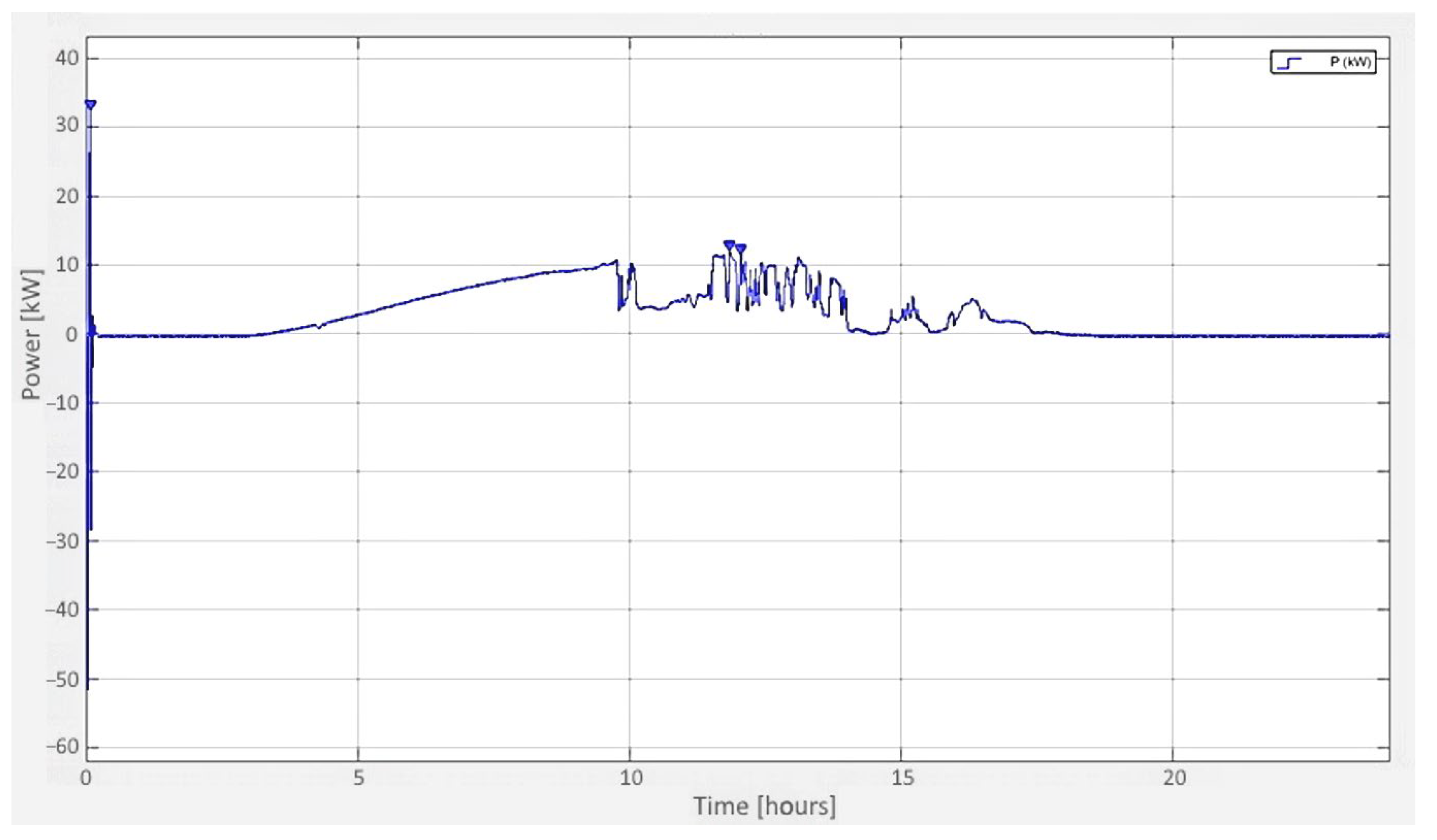
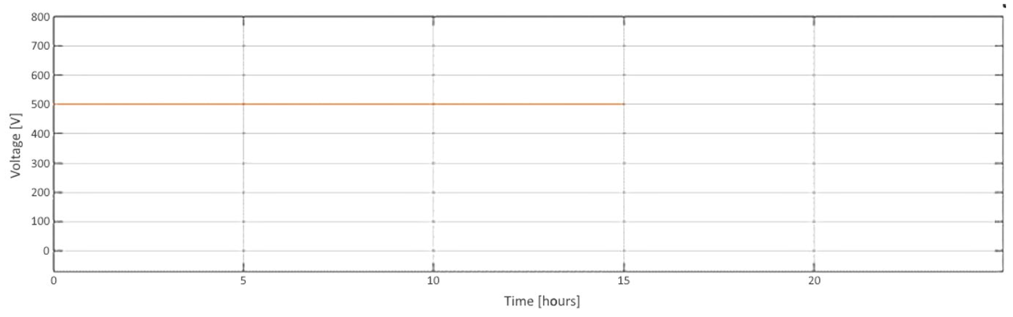
3.1. Simulation of the Operation of Photovoltaic Installations, Viz. the Power and the Average Voltage from the Output of the Modules
- (a)
- Simulation on an exemplary July day for an installation (12.2 kW) comprising 8 strings of 5 panels, 305 W each.
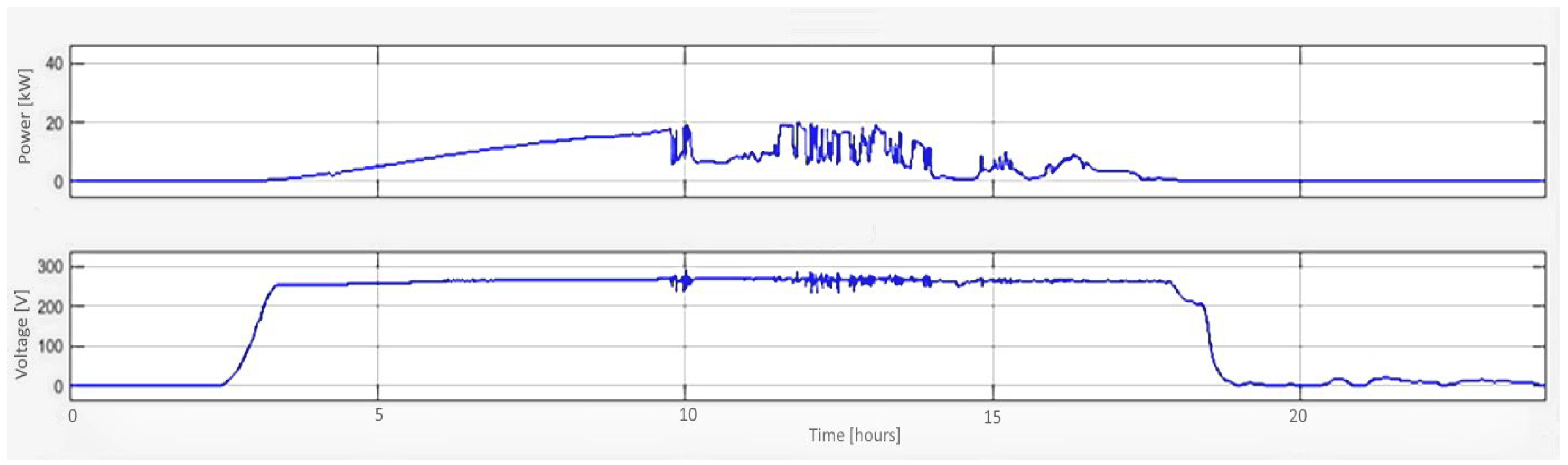
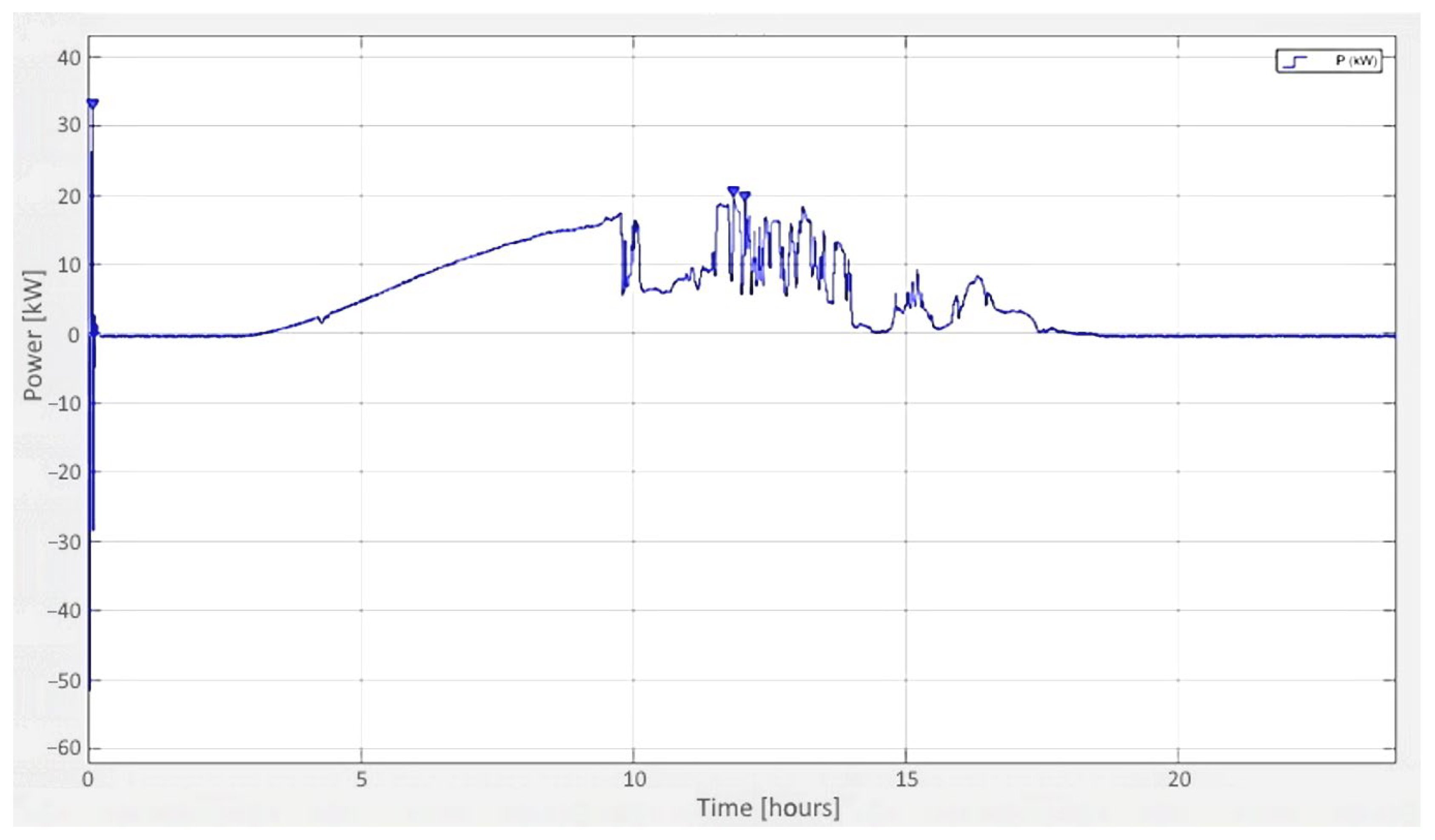
- (b)
- Simulation on a sample day in July for an installation (19.825 kW) comprising 13 strings of 5 panels, 305 W each.
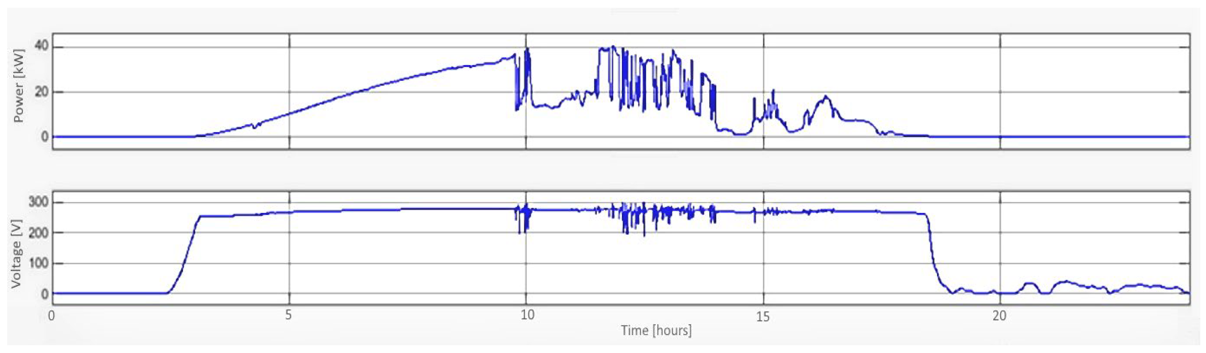
- (c)
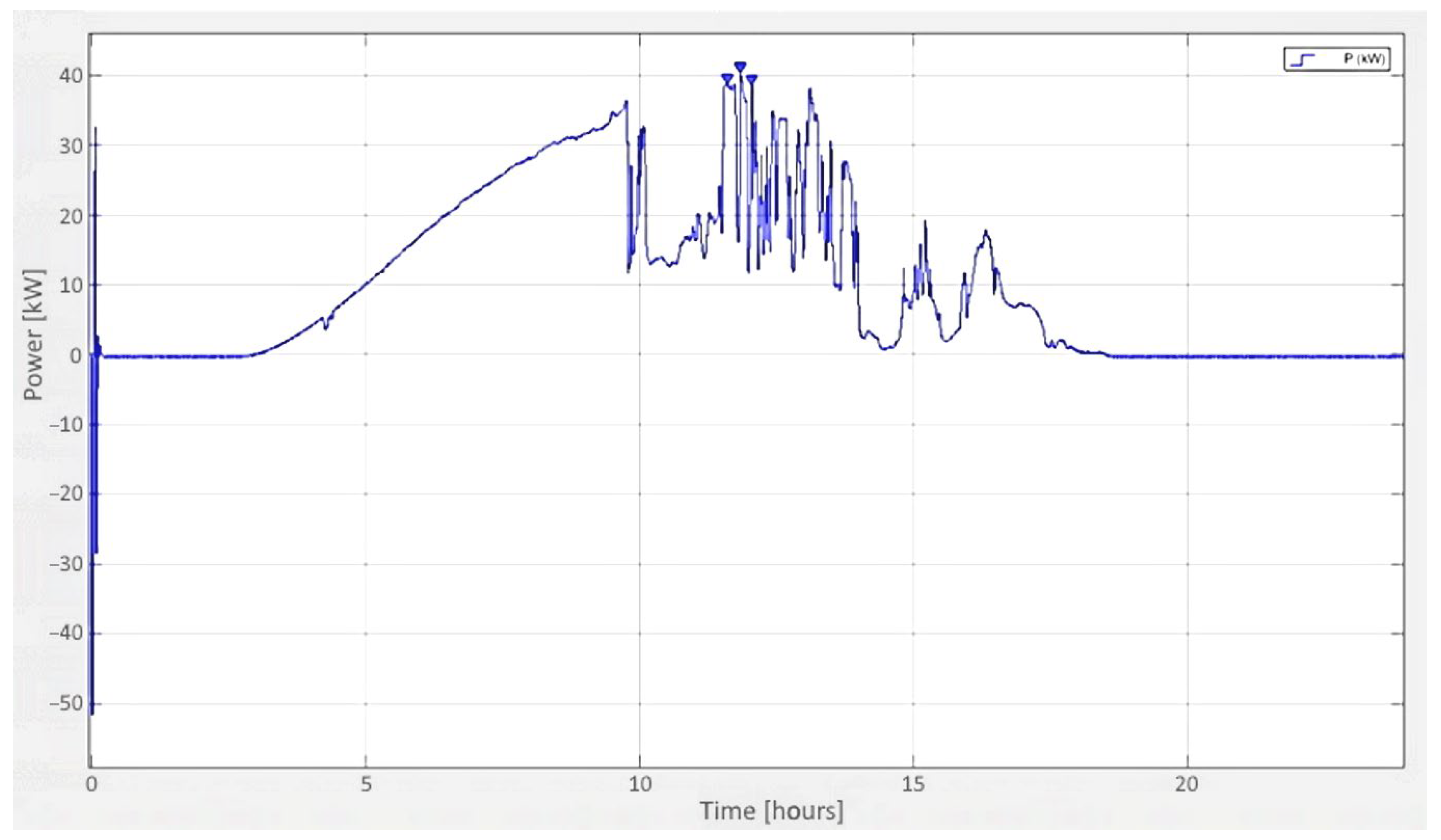
- Simulation on a sample day in July for an installation (39.65 kW) comprising 26 strings of 5 panels, 305 W each.
- (a)
- Simulation on a sample day in July for an installation (12.2 kW) comprising 8 strings of 5 panels, 305 W each.
- (b)
- Simulation on a sample day in July for an installation (19.825 kW) comprising 13 strings of 5 panels, 305 W each.
- (c)
- Simulation on a sample day in July for an installation (39.65 kW) comprising 26 strings of 5 panels, 305 W each.
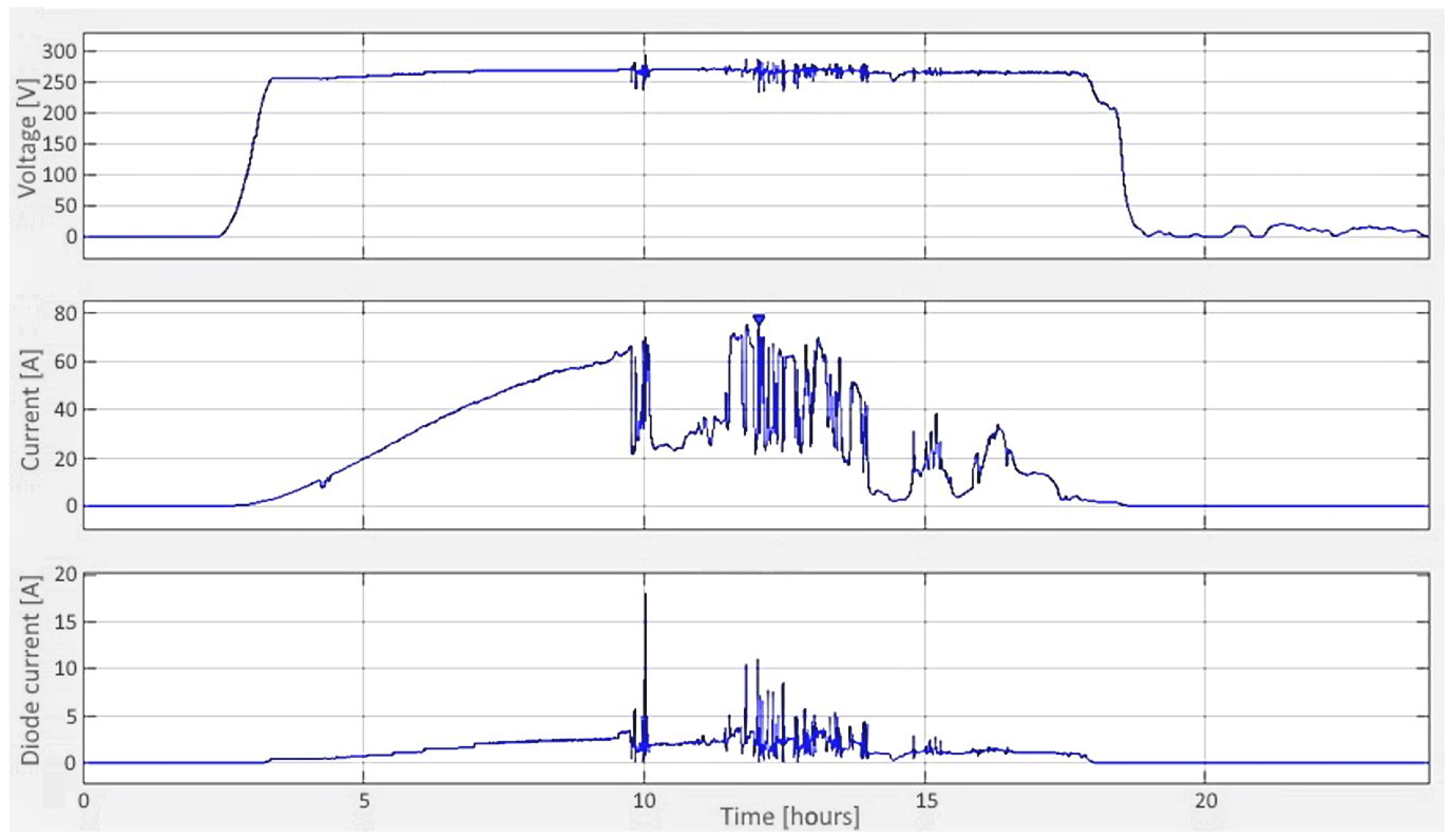
3.2. Simulations of the Parameters of the Power Grid
- (a)
- Simulation on a sample day in July for an installation (12.2 kW) comprising 8 strings of 5 panels, 305 W each.
- (b)
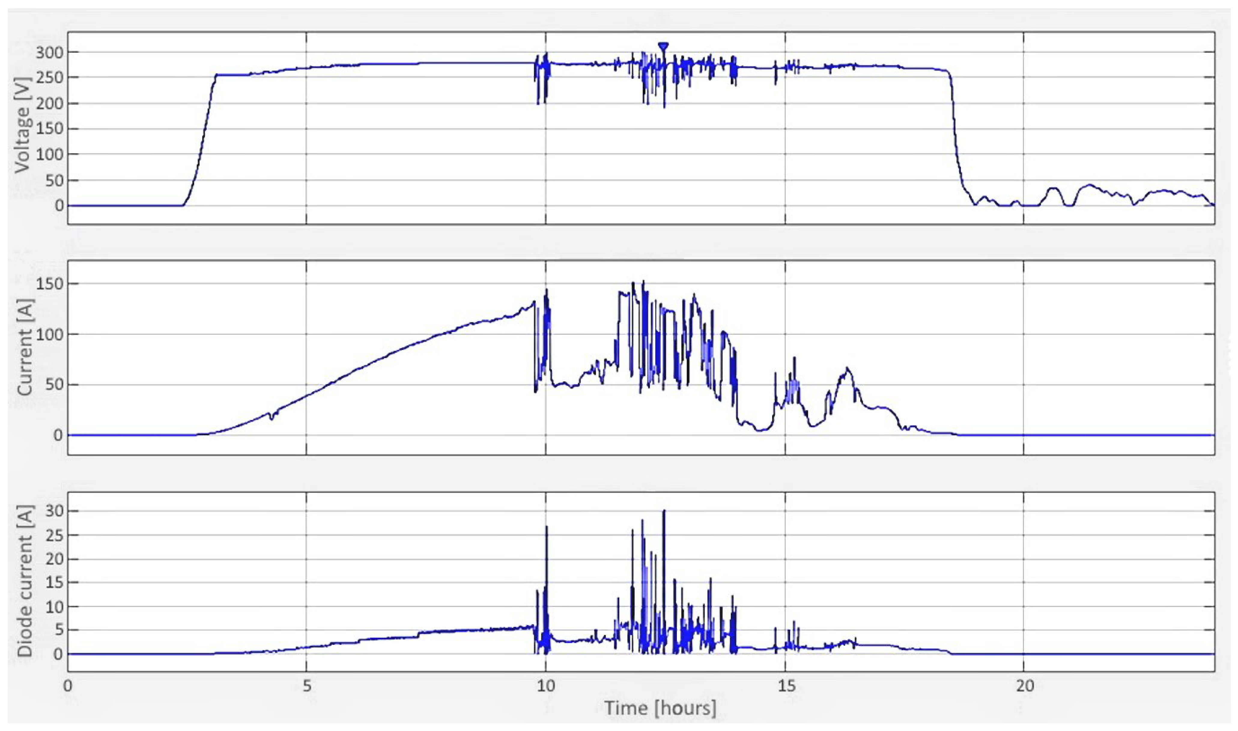
- Simulation on a sample day in July for an installation (19.825 kW) comprising 13 strings of 5 panels, 305 W each.
- (c)
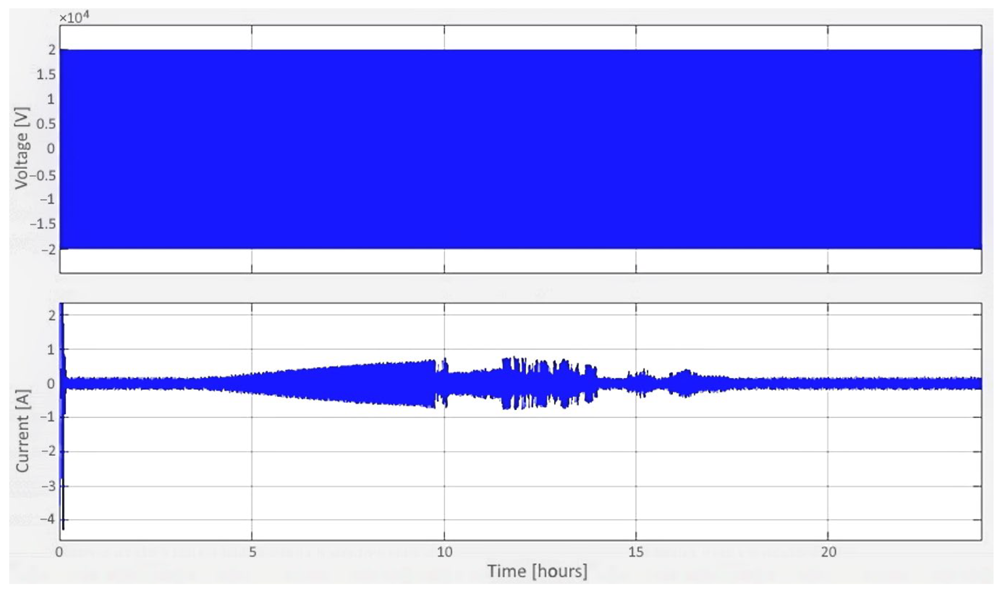
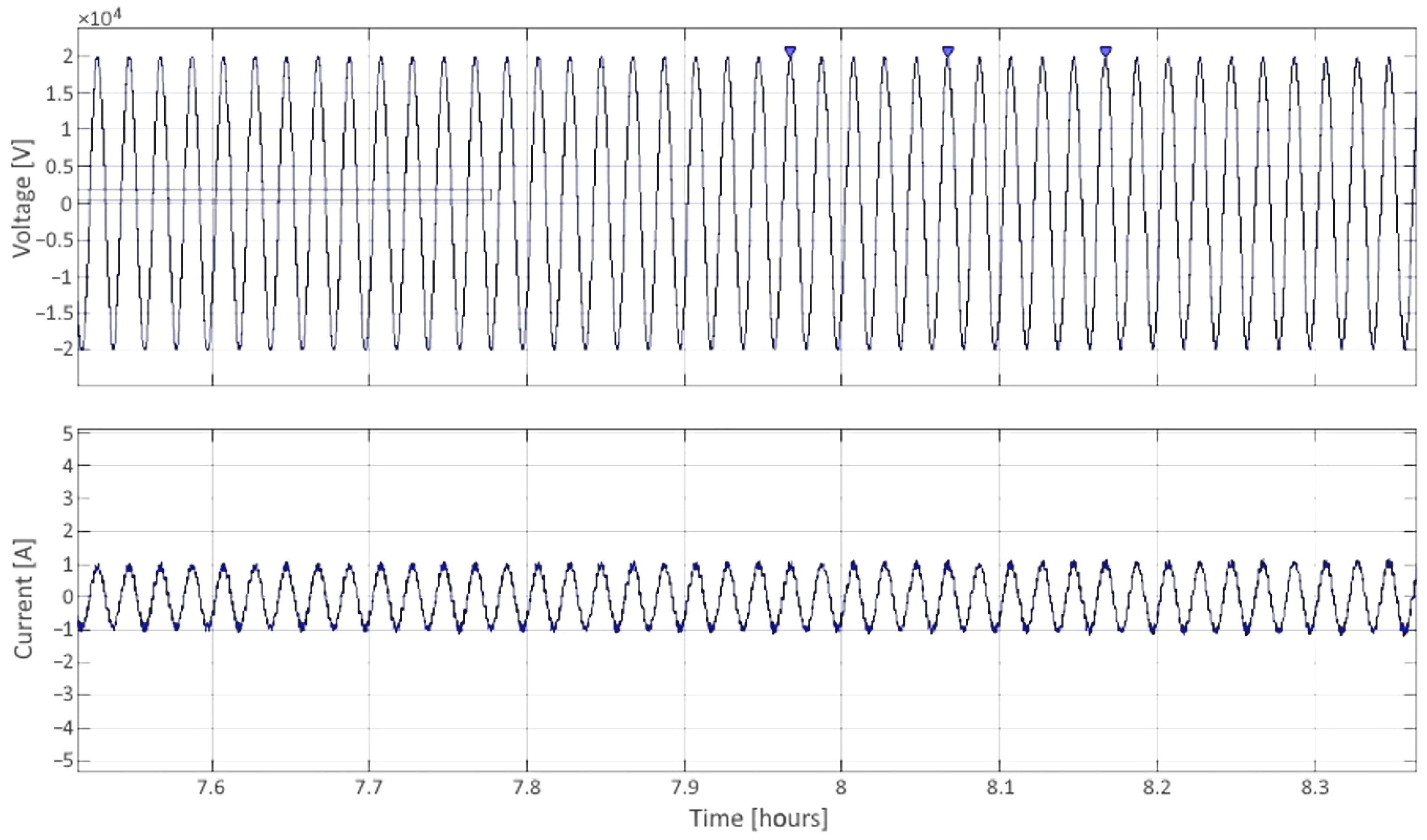
- Simulation on a sample day in July for an installation (39.65 kW) comprising 26 strings of 5 panels, 305 W each.
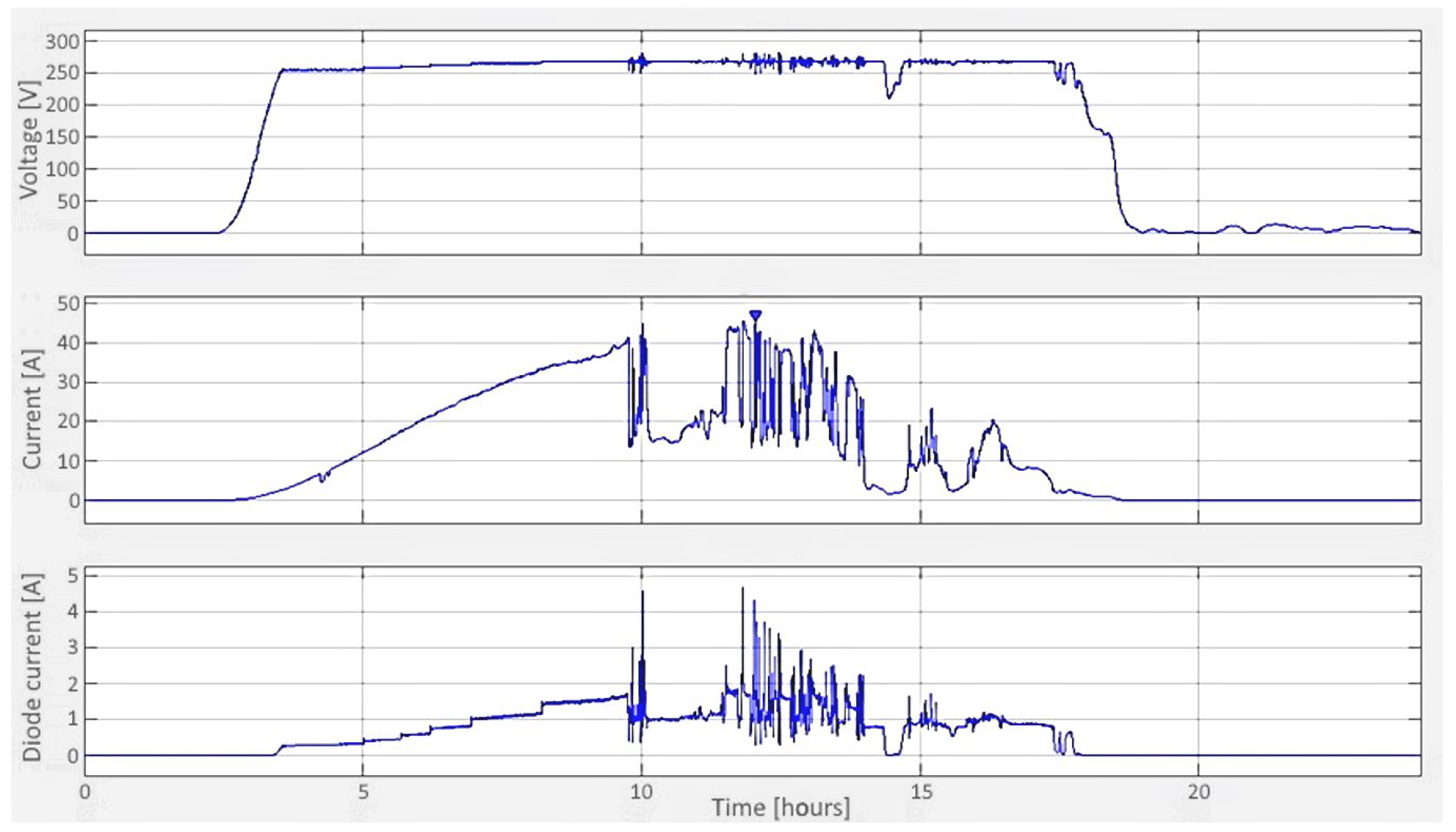
3.3. Discussion of the Simulation Results Obtained for the 39.65 kW Installation
- (a)
- Voltage variations [29]:
- (b)
- Open circuit voltage
- (c)
- Operating voltage
- (d)
- Low temperature operating voltage [29]:
- (e)
- High temperature operating voltage [29]:
- (f)
- Maximum power generated by the panels
- (g)
- Maximum, short-circuit current [19]:
- (h)
- Maximum operating current [19]:
- (i)
- Current and voltage in the power system
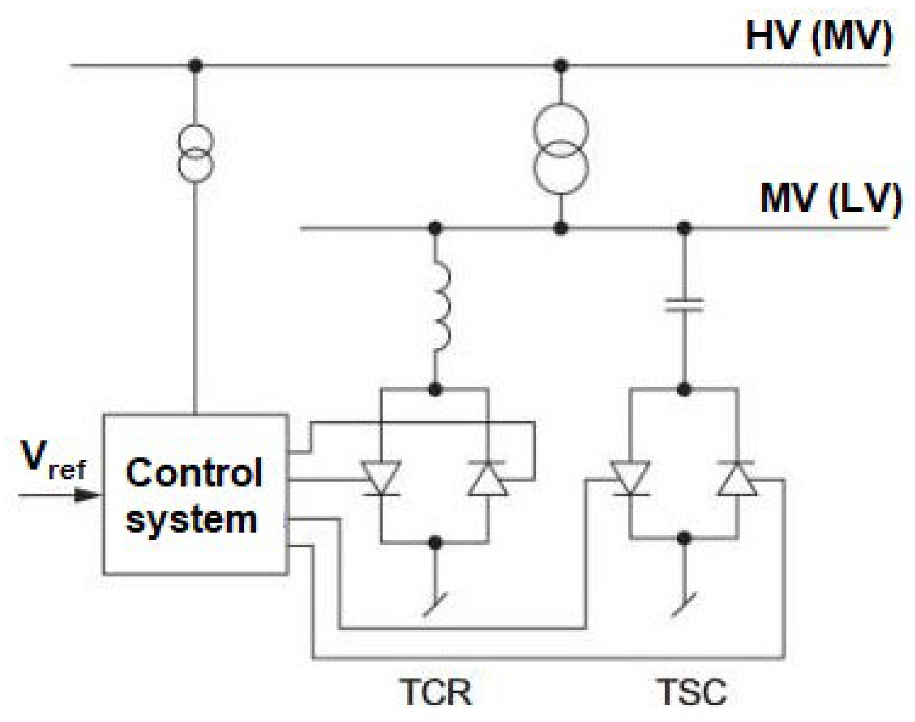
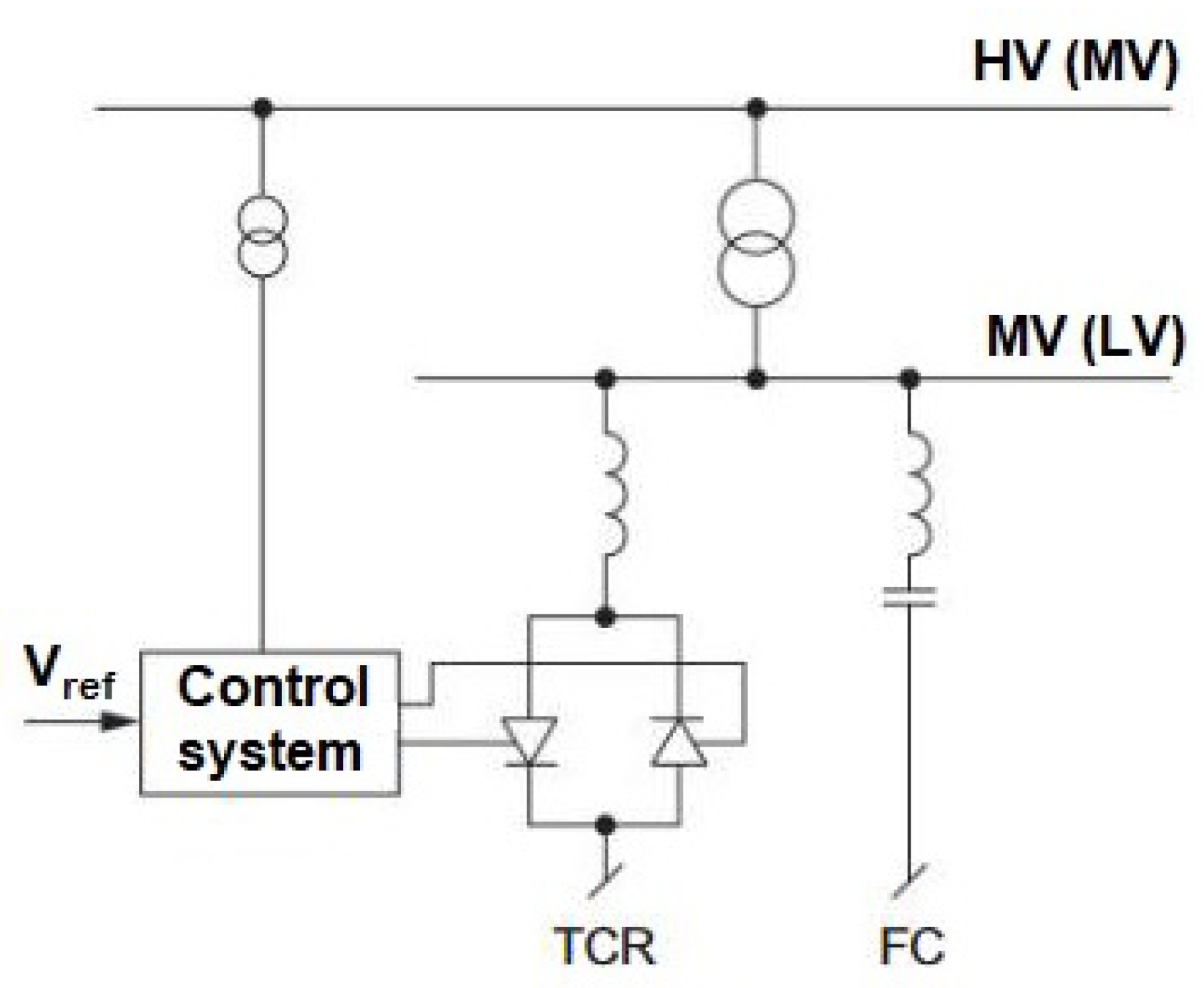
4. Methods for Improving Power Quality
4.1. Compensating for Passive Power
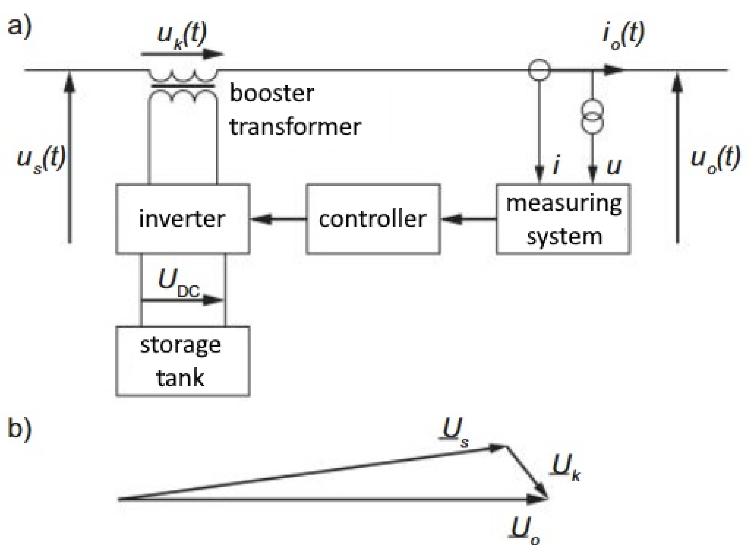
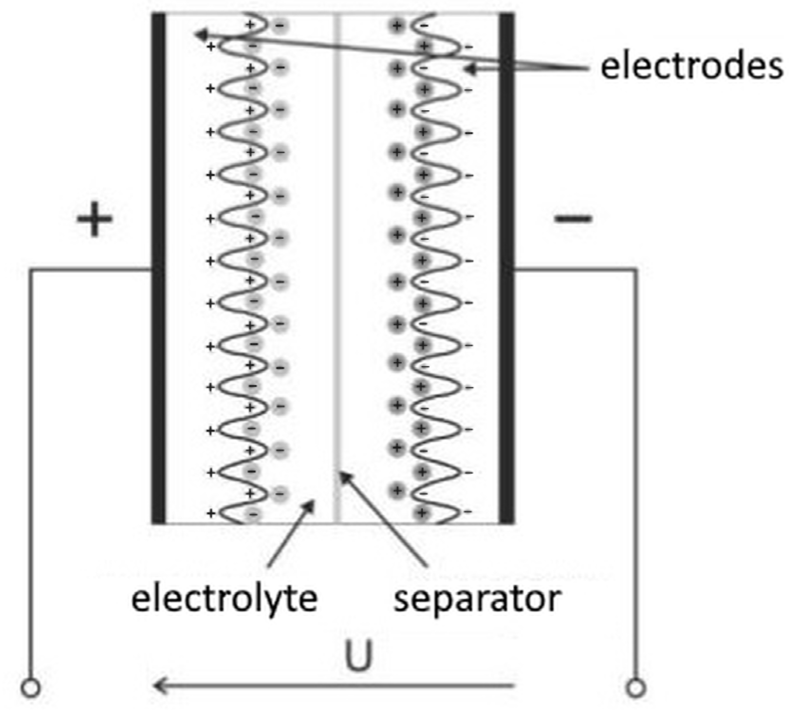
4.2. Possibilities of Using Energy Storage to Improve Power Quality
- Support in the management of active energy, in normal network operation;
- Support for the power supply of receivers during interruptions to the supply network.
5. Conclusions
Author Contributions
Funding
Data Availability Statement
Acknowledgments
Conflicts of Interest
References
- Izdebski, M.; Jacyna, M. An Efficient Hybrid Algorithm for Energy Expenditure Estimation for Electric Vehicles in Urban Service Enterprises. Energies 2021, 14, 2004. [Google Scholar] [CrossRef]
- Urbaniak, M.; Kardas-Cinal, E.; Jacyna, M. Optimization of Energetic Train Cooperation. Symmetry 2019, 11, 1175. [Google Scholar] [CrossRef]
- Jacyna, M.; Golebiowski, P.; Urbaniak, M. Multi-option Model of Railway Traffic Organization Including the Energy Recuperation. In Communications in Computer and Information Science; Springer: Berlin/Heidelberg, Germany, 2016. [Google Scholar] [CrossRef]
- Łuszczyk, M.; Sulich, A.; Siuta-Tokarska, B.; Zema, T.; Thier, A. The Development of Electromobility in the European Union: Evidence from Poland and Cross-Country Comparisons. Energies 2021, 14, 8247. [Google Scholar] [CrossRef]
- Jacyna, M.; Zochowska, R.; Sobota, A.; Wasiak, M. Scenario Analyses of Exhaust Emissions Reduction through the Introduction of Electric Vehicles into the City. Energies 2021, 14, 2030. [Google Scholar] [CrossRef]
- Sweeting, W.J.; Hutchinson, A.R.; Savage, S.D. Factors affecting electric vehicle energy consumption. Int. J. Sustain. Eng. 2011, 4, 192–201. [Google Scholar] [CrossRef]
- Wasiak, M.; Zdanowicz, P.; Nivette, M. Research on the effectiveness of alternative propulsion sources in high-tonnage cargo transport. Arch. Transp. 2021, 60, 259–273. [Google Scholar] [CrossRef]
- Karoń, G. Safe and Effective Smart Urban Transportation-Energy Flow in Electric (EV) and Hybrid Electric Vehicles (HEV). Energies 2022, 15, 6548. [Google Scholar] [CrossRef]
- Karoń, G. Energy Smart Urban Transportation with Systemic Use of Electric Vehicles. Energies 2022, 15, 5751. [Google Scholar] [CrossRef]
- Barchański, A.; Żochowska, R.; Kłos, M. A Method for the Identification of Critical Interstop Sections in Terms of Introducing Electric Buses in Public Transport. Energies 2022, 15, 7543. [Google Scholar] [CrossRef]
- World Cities Report 2022: Envisaging the Future of Cities, United Nations Human Settlements Programme (UN-Habitat); United Nations: New York, NY, USA, 2022.
- Kissa, G.; Jansenb, H.; Castaldoc, V.L.; Orsia, L. The 2050 City. International Conference on Sustainable Design, Engineering and Construction. Procedia Eng. 2015, 118, 326–355. [Google Scholar] [CrossRef]
- Xiang, C.; Matusiak, B.S. Façade Integrated Photovoltaics design for high-rise buildings with balconies, balancing daylight, aesthetic and energy productivity performance. J. Build. Eng. 2022, 57, 104950. [Google Scholar] [CrossRef]
- Anzalchi, A.; Sarwat, A. Overview of technical specifications for grid-connected photovoltaic systems. Energy Convers. Manag. 2017, 152, 312–327. [Google Scholar] [CrossRef]
- Macêdo, W.N.; Zilles, R. Influence of the power contribution of a grid-connected photovoltaic system and its operational particularities. Energy Sustain. Dev. 2009, 13, 202–211. [Google Scholar] [CrossRef]
- Kabiri, R.; Holmes, D.G.; McGrath, B.P. The influence of pv inverter reactive power injection on grid voltage regulation. In Proceedings of the 2014 IEEE 5th International Symposium on Power Electronics for Distributed Generation Systems (PEDG), Galway, Ireland, 24–27 June 2014; pp. 1–8. [Google Scholar] [CrossRef]
- Liu, W.; Peng, D.; Bu, G.Q.; Su, J. A survey on system problems in smart distribution network with grid-connected photovoltaic generation. Power Syst. Technol. 2009, 19, 1–5. [Google Scholar]
- Buzdugan, M. Voltage Dips in Power Quality—A Brief Review. In Proceedings of the 2019 AEIT International Annual Conference (AEIT), Florence, Italy, 18–20 September 2019; pp. 1–6. [Google Scholar] [CrossRef]
- Good, C.; Kristjansdottír, T.; Wiberg, A.H.; Georges, L.; Hestnes, A.G. Influence of PV technology and system design on the emission balance of a net zero emission building concept. Sol. Energy 2016, 130, 89–100. [Google Scholar] [CrossRef]
- Gunduz, H.; Jayaweera, D. Reliability assessment of a power system with cyber-physical interactive operation of photovoltaic systems. Int. J. Electr. Power Energy Syst. 2018, 101, 371–384. [Google Scholar] [CrossRef]
- Zeb, K.; Uddin, W.; Khan, M.A.; Ali, Z.; Ali, M.U.; Christofides, N.; Kim, H.J. A comprehensive review on inverter topologies and control strategies for grid connected photovoltaic system. Renew. Sustain. Energy Rev. 2018, 94, 1120–1141. [Google Scholar] [CrossRef]
- Mróz, M. Wahania napięcia jako kryterium przyłączania elektrowni do sieci dystrybucyjnych. AGH 2018. Available online: http://www.sep.krakow.pl/biuletyn/nbiuletyn/nr61ar2 (accessed on 15 October 2022).
- Jagusiak, M.; Dróżdż, T.; Nawara, P.; Kiełbasa, P.; Lis, S.; Wrona, P.; Nęcka, K.; Oziembłowski, M. Kompatybilność elektromagnetyczna w pomiarach energii elektrycznej. Przegląd Elektrotechniczny 2016, 1, 139–144. [Google Scholar] [CrossRef]
- Pruski, P.; Paszek, S. Analysis of Waveforms in a Power System at Asymmetrical and Symmetrical Short-Circuits in a Transmission Line. Acta Energetica 2019, 1/38, 17–22. [CrossRef]
- Büdenbender, K.; Braun, M.; Schmiegel, A.; Magnor, D.; Marcel, J.C. Improving PV-integration into the distribution grid-contribution of multifunctional PV-battery systems to stabilised system operation. In Proceedings of the 25th European Photovoltaic Solar Energy Conference and Exhibition, Valencia, Spain, 6–10 September 2010; pp. 4839–4845. [Google Scholar]
- de Silva, G.D.O.; Hendrick, P. Photovoltaic self-sufficiency of Belgian households using lithium-ion batteries, and its impact on the grid. Appl. Energy 2017, 195, 786–799. [Google Scholar] [CrossRef]
- de Lima, L.C.; de Araújo Ferreira, L.; de Lima Morais, F.H.B. Performance analysis of a grid connected photovoltaic system in northeastern Brazil. Energy Sustain. Dev. 2017, 37, 79–85. [Google Scholar] [CrossRef]
- Bouacha, S.; Malek, A.; Benkraouda, O.; Arab, A.H.; Razagui, A.; Boulahchiche, S.; Semaoui, S. Performance analysis of the first photovoltaic grid-connected system in Algeria. Energy Sustain. Dev. 2020, 57, 1–11. [Google Scholar] [CrossRef]
- Sharma, R.; Goel, S. Performance analysis of a 11. 2 kWp roof top grid-connected PV system in Eastern India. Energy Rep. 2017, 3, 76–84. [Google Scholar] [CrossRef]
- Detailed Model of a 100-kW Grid-Connected PV Array. Available online: https://www.mathworks.com/help/physmod/sps/ug/detailed-model-of-a-100-kw-grid-connected-pv-array.html (accessed on 26 January 2022).
- Moacyr, A.G.; de Brito, L.P.; Sampaio, L.G., Jr.; e Melo, G.A.; Canesin, C.A. Comparative Analysis of MPPT Techniques for PV Applications. In Proceedings of the 2011 International Conference on Clean Electrical Power (ICCEP), Ischia, Italy, 14–16 June 2011. [Google Scholar] [CrossRef]
- Kjaer, S.B.; Pedersen, J.K.; Blaabjerg, F. Power inverter topologies for photovoltaic modules-a review. In Proceedings of the 2002 IEEE Industry Applications Conference. 37th IAS Annual Meeting (Cat. No. 02CH37344), Pittsburgh, PA, USA, 13–18 October 2002; Volume 2, pp. 782–788. [Google Scholar] [CrossRef]
- Mehiri, A.; Bettayeb, M.; Hamid, A.K.; Ardjal, A. Fractional nonlinear synergetic control for DC-link voltage regulator of three phase inverter grid-tied PV system. In Proceedings of the 5th International Conference on Renewable Energy: Generation and Applications (ICREGA), Al Ain, United Arab Emirates, 25–28 February 2018. [Google Scholar]
- SPR-305E-WHT-D Solar Panel from SunPower. Available online: https://www.posharp.com/spr-305e-wht-d-solar-panel-from-sunpower_p1621616600d.aspx,11.2022 (accessed on 10 November 2022).
- Kowalak, R.; Malkowski, R.; Czapp, S.; Klucznik, J.; Lubosny, Z.; Dobrzynski, K. Computer-aided analysis of resonance risk in power system with Static Var Compensators. Prz. Elektrotechniczny 2016, 1, 22–27. [Google Scholar] [CrossRef] [PubMed]
- Kubek, P.; Rzepka, P.; Szablicki, M.; Wasilewski, J. Electric Energy Storages—An Innovative Idea for Frequency Stabilization in Power System. Autom. Electrotech. Disturb. 2016, 7, 6–11. [Google Scholar] [CrossRef]


| Date | Number of Chains Containing 5 Modules Each, with a Power of 305 W Each | Theoretical | Theoretical |
|---|---|---|---|
| 8 | 12.20 | 12.30 | |
| 18 July 2021 | 13 | 19.83 | 19.96 |
| 26 | 39.65 | 38.90 |
| Parameter | [V] | |||
|---|---|---|---|---|
| Maximum value | 281.8 | 282 | 45.87 | 4.698 |
| Time of occurrence of the maximum value | 12:26 | 12:26 | 12:03 | 11:44 |
| Minimum value | 0 | 0 | −5.996∙10−10 | 0 |
| Time of occurrence of the minimum value | 20:46 | |||
| Mean value | 169.9 | 168.3 | 11.65 | 0.5695 |
| Median | 257.6 | 257.6 | 5.741 | 0.4144 |
| Parameter | [V] | |||
|---|---|---|---|---|
| Maximum value | 292.6 | 292.9 | 75.31 | 18.05 |
| Time of occurrence of the maximum value | 10:01 | 10:01 | 12:01 | 10:02 |
| Minimum value | 0 | 0 | −2∙10−10 | 0 |
| Time of occurrence of the minimum value | 172.7 | 20:48 | ||
| Mean value | 172.7 | 260.2 | 18.84 | 1.011 |
| Median | 260.2 | 9.457 | 0.8382 |
| Parameter | [V] | |||
|---|---|---|---|---|
| Maximum value | 293.2 | 301.6 | 154.5 | 31.67 |
| Time of occurrence of the maximum value | 12:28 | 12:27 | 12:03 | 12:27 |
| Minimum value | 0 | 0 | −8.71∙10−10 | 0 |
| Time of occurrence of the minimum value | 181.8 | 181.8 | 20:41 | |
| Mean value | 267.5 | 176.7 | 37.63 | 2.083 |
| Median | 260 | 19.05 | 1.325 |
| Date | Number of Chains with 5 Modules Each, with a Power of 305 W Each | [kV] | [kV] | [A] | [A] |
|---|---|---|---|---|---|
| 8 | 19.91 | −19.93 | 4.078 | −4.287 | |
| 18 July 2021 | 13 | 19.90 | −19.89 | 4.078 | −4.287 |
| 26 | 19.91 | −19.93 | 4.078 | −4.287 |
| Parameter | [kW] | [V] | ||||||
|---|---|---|---|---|---|---|---|---|
| Maximum value | 38.90 | 293.2 | 301.6 | 154.5 | 31.67 | 38.64 | 19,910 | 4.078 |
| Time of occurrence of the maximum value | 11:48 | 12:28 | 12:27 | 11:52 | 12:27 | 11:54 | 00:04 | |
| Minimum value | 0 | 0 | 0 | −8.71∙1010 | 0 | −51.5 | −19,930 | −4.287 |
| Time of occurrence of the minimum value | 8:41 | 00:06 | 00:07 | |||||
| Mean value | 10.31 | 181.8 | 176.7 | 37.63 | 2.083 | 9.61 | 0.00083 | |
| Median | 50.52 | 267.5 | 260 | 19.05 | 1.352 | 4.62 | 0.00079 |
| Area of Application | Functions of the Storage | Purpose of the Storage/Results Obtained |
|---|---|---|
| Electricity grid | co-operation with RES |
|
| load balancing |
| |
| voltage regulation and compensation for electromagnetic interruptions | improving the quality of the electricity | |
| Final recipient | supplying receivers during voltage dips and interruptions to the power supply | reducing the cost of losses resulting from dips and interruptions to the power supply |
| storing energy, in periods of low demand in the system and providing energy to the recipient in periods of maximum demand | reducing the amount of energy consumed from the grid, during periods of maximum demand; reducing energy bills | |
| Prosument | load balancing | limiting energy consumption from the power grid |
| voltage regulation and compensation for electromagnetic interruptions | improving the quality of the electricity | |
| supplying receivers during voltage dips and interruptions to the power supply | reducing the cost of losses resulting from dips and interruptions to the power supply |
Disclaimer/Publisher’s Note: The statements, opinions and data contained in all publications are solely those of the individual author(s) and contributor(s) and not of MDPI and/or the editor(s). MDPI and/or the editor(s) disclaim responsibility for any injury to people or property resulting from any ideas, methods, instructions or products referred to in the content. |
© 2023 by the authors. Licensee MDPI, Basel, Switzerland. This article is an open access article distributed under the terms and conditions of the Creative Commons Attribution (CC BY) license (https://creativecommons.org/licenses/by/4.0/).
Share and Cite
Chamier-Gliszczynski, N.; Trzmiel, G.; Jajczyk, J.; Juszczak, A.; Woźniak, W.; Wasiak, M.; Wojtachnik, R.; Santarek, K. The Influence of Distributed Generation on the Operation of the Power System, Based on the Example of PV Micro-Installations. Energies 2023, 16, 1267. https://doi.org/10.3390/en16031267
Chamier-Gliszczynski N, Trzmiel G, Jajczyk J, Juszczak A, Woźniak W, Wasiak M, Wojtachnik R, Santarek K. The Influence of Distributed Generation on the Operation of the Power System, Based on the Example of PV Micro-Installations. Energies. 2023; 16(3):1267. https://doi.org/10.3390/en16031267
Chicago/Turabian StyleChamier-Gliszczynski, Norbert, Grzegorz Trzmiel, Jarosław Jajczyk, Aleksandra Juszczak, Waldemar Woźniak, Mariusz Wasiak, Robert Wojtachnik, and Krzysztof Santarek. 2023. "The Influence of Distributed Generation on the Operation of the Power System, Based on the Example of PV Micro-Installations" Energies 16, no. 3: 1267. https://doi.org/10.3390/en16031267
APA StyleChamier-Gliszczynski, N., Trzmiel, G., Jajczyk, J., Juszczak, A., Woźniak, W., Wasiak, M., Wojtachnik, R., & Santarek, K. (2023). The Influence of Distributed Generation on the Operation of the Power System, Based on the Example of PV Micro-Installations. Energies, 16(3), 1267. https://doi.org/10.3390/en16031267