Article

Investigation on the Mobile Wheeled Robot in Terms of Energy Consumption, Travelling Time and Path Matching Accuracy

Faculty of Electrical Engineering, Częstochowa University of Technology, 17 Armii Krajowej Avenue, 42-201 Częstochowa, Poland
*
Author to whom correspondence should be addressed.
Energies 2023, 16(3), 1210; https://doi.org/10.3390/en16031210
Submission received: 9 December 2022 / Revised: 28 December 2022 / Accepted: 17 January 2023 / Published: 22 January 2023
(This article belongs to the Special Issue Improvements of the Electricity Power System II)

Abstract

:
The task of controlling a wheeled mobile robot is an important element of navigation algorithms. The control algorithm manages the robot’s movement in accordance with the path determined by the planner module, where the accuracy of mapping the given route is very important. Most often, mobile robots are battery-powered, which makes minimizing energy consumption and shortening travel time an important issue. For this reason, in this work, the mobile robot control algorithm was tested in terms of energy consumption, travel time and path mapping accuracy. During the research, a criterion was developed, thanks to which it was possible to select the optimal parameters of the pure pursuit algorithm that controls the movement of the tested robot. The research was carried out in the Laboratory of Intelligent Mobile Robots using the QBot2e mobile robot operating on the basis of differential drive kinematics. As a result of the research, optimal values of the control parameters were obtained, minimizing the travel time, energy consumption and mapping error of the given paths.

1. Introduction

1.1. Power Supply Systems for Mobile Robots

Mobile robots operate with limited energy resources, which are mainly used for movement. In addition, power is required for individual logical components or sensors that are equipped with the robot. Skillful control and directing energy to individual components allows you to reduce wear and extend the robot’s operation on a single battery charge. The development of mobile robotics and the related limitations in access to energy force the optimization of electricity consumption. Movement algorithms aimed at minimizing energy consumption were studied. Much research has been done to find the optimal scheduling methods [1,2,3,4,5,6,7]. The issues related to it are also extremely important in the case of electric vehicles. A large group of solutions are those based on machine learning [8,9] The article [10] presents an overview of how to approach this problem. The decision-making strategy and path-planning algorithms for various types of robots are described. Techniques presenting a classic, heuristic, AI-based or biology-inspired approach were classified. Regardless of the technique used, the route planning criteria are equally important. Depending on the desired results, these criteria may change. Traditional planning of the optimal path of the robot mainly takes into account distance and time criteria [11]. Therefore, the path planned in this way will not always be optimal in terms of energy. Research is also carried out on the cost function of algorithms that take into account information about the environment by introducing a criterion related to energy [12,13]. In the work [14], the ways of moving the robot were examined, taking into account, among others, engine dynamics and a 3-stage speed profile. Energy savings of up to 30% have been demonstrated using different profiles.
Another aspect is research related to the dynamic assessment of the effective capacity of the battery, its discharge rate, and especially the energy needed to reach the charging station by the robot. In [15], the authors proposed a method of energy management by assessing the risk of battery depletion. Risk assessment can replace a fixed, configurable parameter, the exceeding of which determines the return of the robot to the charging station. Such management means that the decision to redirect the robot to the station may be a compromise between the risk and the level of mission implementation. The method can be used to assess the legitimacy of undertaking a mission and its completion at a certain level of battery charge. This issue can be used especially in the case of cleaning robots.
Scientific research is also focused on planning the robot’s trajectory, taking into account optimal energy consumption. An example is the work [16], which uses the theory of optimal control with a cost function determined by the total energy drawn from the batteries. The presented method resulted in energy savings of up to 4.3% compared to the widely used trapezoidal velocity profile. The same authors, in [17], presented a trajectory planning algorithm that allows saving up to 4.75% of energy in relation to the trapezoidal velocity profile.
In [18], the authors proposed a model of energy consumption by a wheeled robot, which was confirmed experimentally. This model and motion planning method were used to minimize the energy consumption of the moving robot.
Subsequent works by the authors were published in the article [19], a new, optimal approach to traffic planning was proposed, consisting of the use of the A algorithm enriched with the energy saving criterion. The time and speed of reaching the next waypoints were optimized.
Energy saving is equally important when planning the flight path of multi-copters. For instance, in [20] it was proposed an algorithm for finding an energy-efficient path between two points in three-dimensional space. The authors conducted simulations and experimental studies confirming the reduction of energy consumption after applying the algorithm compared to the traditional line-of-sight-based path planning. Modern technologies are also based on the Battery Management System (BMS). Algorithms are developed and verified in laboratory conditions, presenting the idea of a BMS system using the Kalman filter [21].

1.2. The Criteria of the Path Matching Accuracy

Recently, there has been a noticeable increase in the availability of devices that can be used to track moving objects. Among them are GPS devices. The result is an increase in traffic data [22]. Moving objects include cars, animals, hurricanes, athletes, mobile users and data packets. Objects can be divided into spatial objects and non-spatial objects. Spatial objects include for example, cars that change their position over time, while non-spatial objects include, for example, time series [22]. A set of data about a moving object is generated at a large scale and at a pace in almost every area of life. An example of this may be data collected from updating the position of a moving object in location services, analyzing stock market trends or speech recognition. As a result, there is a noticeable growing interest in new proposals for grouping, classification, indexing and measuring similarity data for moving objects [22,23].
There are many different methods of measuring curve similarity that have been explored in the field of computational geometry. Similarity measures can be divided into spatial-temporal similarity measures and spatial similarity measures. Spatial-temporal similarity measures take into account both the temporal and spatial dimensions when measuring trajectory similarity. Distance measurements between trajectories are based on aligning the ith element of the first trajectory with the ith element of the second trajectory. The remaining elements, in this case, allow for a local shift in time for better similarity. A local time shift is performed when you move one trajectory element along the time axis to match another trajectory. Both of these elements can appear at different positions of the trajectory. Among the measures of spatial and temporal similarity, [22,23] should be mentioned:
  • Movement speed similarity using time. In this method, position information is separated from time information in such a way that the movement of the object is represented by velocity curves and path curves. The adopted warping approach allows the data points in the sequences to be brought closer together. This approach is repeated and the elements are moved around for a better fit. By separating information about position and time, it is possible to select the path, and speed separately or together to measure probability. As a result of this approach, it is possible to find similarities between trajectories of different lengths. However, this approach is not immune to interference [22].
  • Similarity measure based on time series. This method is a sequence of sampled values over a specific period of time. Individual time series data can be normalized by reducing the data range. This is necessary to keep the distance of the trajectory in relation to scaling and spatial shifting constant. These types of measures are usually related to the distance function, which in turn can be metric or non-metric. With a local offset, the two time series are aligned for better similarity with fewer deletions and fewer insertions and matches. One removal of an element from the first time series results in an insertion into the second, and the inserted element is called a gap element. The downside of this method is the constant penalty for gaps when using the delete and insert operations.
  • The spatial similarity measure group considers only the spatial dimension. In this case, the time dimension is completely omitted. Similarity measures fall into two categories: similarity based on actual values and similarity based on the geometric shape of the trajectory. Spatial similarity measures include among others [22]:
    Euclidean distance. This is a metric measure, also known as the L 2 norm. This norm assumes that every ith point in the first sequence is aligned with the ith point in the second sequence. Local time is not considered in this case. In this method, it is not possible to find similarities for trajectories of different lengths, and it is not immune to interference.
    Angular similarity metric or shape (AMSS). This is a non-metric measure of similarity that treats a single time series as a vector sequence for better handling of spatial variability. Here, the similarity between two vector sequences is calculated based on the directions of the vectors. The location of the actual data points in space is not taken into account. This method takes into account the shift in time and also allows you to find similarities in trajectories of different lengths.
    Hausdorff and Frechet distance. This method was used in the presented research. The Hausdorff distance is a metric measure that measures the distance of one shape of one trajectory is close to the distance of another shape of the next trajectory. In this method, for each shape point of the first trajectory, the distance to the nearest shape point of the second trajectory is taken into account. The Frechet distance, on the other hand, is a non-metric measure. It takes into account the location and order of points along the curves of the trajectory shapes. The shift of the time dimension is not taken into account here. These methods are not immune to interference. In addition, the two compared curves may have different lengths, i.e., the number of vertices [23].
Work is also being carried out on planning the robot to move faster while ensuring collision-free operation. One way is to reduce the processing time of algorithms [24,25]. An important issue is also the accuracy of the path mapping, methods related to planning the most accurate path can be found in [26,27,28].
The article proposes a criterion that allows you to link these criteria with each other and, depending on the needs, use one or several of them to assess the robot’s journey and the resources used. It will also be possible to introduce weights, which will increase the importance of individual parameters.
The remaining sections of the paper are organized as follows. In Section 2, experimental setup and research methodology are described. In Section 3, the results of hardware in the loop experiments with a mobile robot QBot 2e is presented. A discussion of the results regarding the selection of optimal control parameters in terms of energy consumption, travel time and path matching accuracy is introduced in Section 4. Finally, Section 5 is a summary of our conclusions.

2. Materials and Methods

2.1. Mobile Wheeled Robots

In recent years, there has been a significant increase in the development of technologies related to the control and communication of mobile robots. One of the fastest growing branches of robotics are mobile robots, which have a high ability to move in land, air and water space [29]. Such robots can be controlled remotely by a human or can be used as autonomous units. Depending on the mobility system used, robots can be divided into: wheeled, walking, underwater and other [30]. Wheeled mobile robots are used in many areas of life, from simple household tasks such as cleaning, to specialized work such as work in a contaminated environment [31,32]. To improve communication between robots and enable them to work autonomously, newer solutions are being developed. Robots are equipped with appropriate tools that allow them to perform the tasks that are set before them. The implementation is supported by various locators such as GPS, vision systems and other additional sensors. The important issue related to mobile robotics systems is the control algorithm. There are many algorithms that are strictly linked with the given kinematic model.
The study of the control algorithm described in the later part of the work was carried out using the QBot2e mobile robot. The way the robot moves can be described using the equations of direct and inverse kinematics of the differential drive [33,34]. Simple kinematics allows determining the linear velocity v c and the angular rate ω c of the mobile platform based on the linear velocities of the right and left wheels denoted by v R and v L , respectively. In the further part of the work, the following model of simple kinematics was adopted in relation to the global coordinate system [33,35,36,37]:
x ˙ y ˙ Θ ˙ = 1 2 v R + v L cos Θ 1 2 v R + v L sin Θ 1 d v R v L ,
where v L , v R , m/s—linear velocities of the left and right wheels, respectively; v c , m/s—linear speed of the mobile platform; d, m—distance between wheels; Θ , rad—angle of rotation of the mobile platform relative to the O X axis around the axis perpendicular to the O X Y plane; x , y —coordinates of the center of the mobile platform describing the position of the robot.
From the point of view of control tasks, in particular reproducing the path by a wheeled robot, it is necessary to determine the linear speeds of the wheels v R and v L on the basis of the values of the linear speed v c and the angular ω c of the mobile platform, set by the regulator. This is the inverse problem of Equation (1) and is called the inverse kinematics model. In the case of the tested robot, the inverse kinematics model is expressed by the equation:
v R v L = v c + 1 2 d ω c v c 1 2 d ω c .
Various methods can be used to control the motion of the robot [38,39], including geometric path-tracking algorithms [40], classical control algorithms [39], or optimal control methods [41,42]. In this article, the problem of motion control has been defined as the problem of following a path given in the form of a set of waypoints. Two of them were distinguished as the starting and ending points, with the set value being the position of the robot, without taking into account its speed or orientation. The pure pursuit [43] algorithm was used for the control defined in this way. This algorithm allows the robot to follow a specific trajectory. For this purpose, the algorithm in each time step calculates the curvature of the vehicle track required to reach the next waypoint of the given route. The first input parameter of the control algorithm is the vector of the positions of the waypoints of the given trajectory (points that the robot should visit). The second data is the look-ahead parameter, defined as a constant distance between the robot’s current position and the current target point on the path defined by given points [40,43]. As mentioned above, the algorithm computes the curvature such that each step of the algorithm allows the vehicle to travel from the current point to the instantaneous destination point. As a result of the algorithm, the robot moves in pursuit of a fleeing temporary destination along the path. In this way, the vehicle reproduces the curvature of the predetermined path. To increase the quality of control, in this work, in the pure pursuit algorithm, a given linear velocity was adopted and an additional limit was imposed on the maximum value of the angular velocity.

2.2. Experimental Setup

Experimental research was carried out in the Laboratory of Intelligent Mobile Robots built at the Faculty of Electrical Engineering of the Częstochowa University of Technology. The hardware and software resources included in the stand were used, enabling scientific research to be carried out using the QBot2e [44] wheeled robot. The basic elements of the experimental setup are [45]:
  • Control station consisting of a central unit (PC computer) with software installed: Matlab 2019a, QUARC Real-Time Control Software 2018, Motive 2.0, Visual Studio Community Compiler 2017.
  • Two QBot 2e mobile robots.
  • Eight Optitrack Flex 13 cameras used to track the position of mobile robots.
  • Additional accessories enabling, e.g., communication between the elements of the station.
In addition, a secured space with dimensions of 5 m × 5 m × 2.5 m is prepared, in which mobile robots move. Inside the cage prepared in this way, under the ceiling, there are cameras tracking the position of the robot. Figure 1 shows a top view of the OptiTrack system cameras arrangement in the working space. The cameras are located near the ceiling and evenly distributed around the workspace. A number is assigned to each camera, thanks to which it is possible to quickly locate it both in reality and in the application cooperating with the cameras.
Data from the cameras are sent to the Matlab environment. The communication process is managed by an optical motion capture application—Motive 2.0. The cameras record images with Resolution 1280 × 1024 , Native Frame Rate—120 Hz, Shutter Default Speed 0.25 ms, 3D Accuracy +/− 0.20 mm. The presented parameters of the cameras make it possible to locate the robot with an accuracy of 1 millimeter. The OptiTrack system tracks robots by installing special markers on them. The arrangement of markers on each tracked robot must be unique so that the software correctly identifies the object. The layout of robot markers must also be entered in the Motive application, where markers representing a given object are grouped and a rigid body representing the robot [45] is created.
Carrying out the tests is always associated with the calibration [35]. For this purpose, the relative position of the cameras in space and their location relative to the ground should be determined. The calibration uses the CW-500 calibration wand and the CS-200 calibration ground square. As a result of the calibration process, two configuration files are created, which are used by the control algorithms developed in the MATLAB Simulink [45] environment. The OptiTrack system works in real-time with the MATLAB Simulink environment. Thanks to this, it is possible to record the position of the robot in real-time from the Simulink block diagram and perform HIL (hardware in the loop) simulations. As part of the research, a simulation scheme was created that allows locating the robot thanks to cooperation with the Motive application.
The OptiTrack object tracking system presented above is a hardware and software platform that creates the Motion Capture System. Thanks to this technology, it is possible to record the position of objects in real-time. It finds many applications in the modern world, both civilian and military. This technology, depending on the method of tracking markers, can be divided into three groups: optical-passive, optical-active and video [35,46]. Optical-passive technology is used in the Laboratory of Intelligent Mobile Robots.
The control of mobile robots is carried out using models developed in the Matlab/Simulink environment using dedicated QUARC blocks. Two models are used simultaneously. These models are run on two targets.
The target is a set of software tools. It allows, in particular, to run compiled hardware in the loop (HIL) programs in a specific operating system environment. In addition, the target enables the communication between the compiled Simulink diagram and the diagram in which the HIL simulation is performed. Two targets of the Simulink/QUANSER environment were used in this work. One of the targets was launched at the control station. It was used to simulate HIL. The second target was installed on a Raspberry Pi minicomputer integrated with the QBot 2e robot. It was used to directly control the movement of the robot.
In addition, the PoseTracker.slx model was launched on the workstation during the simulation. He was responsible for communication of the Matlab/Simulink environment with the OptiTrack system (tracking the position of a mobile robot using motion capture technology). Thanks to this, information about the position of the robot was saved in real-time on the workstation disk. This model contains standard blocks of communication with the OptiTrack system, data conversion and saving [35].
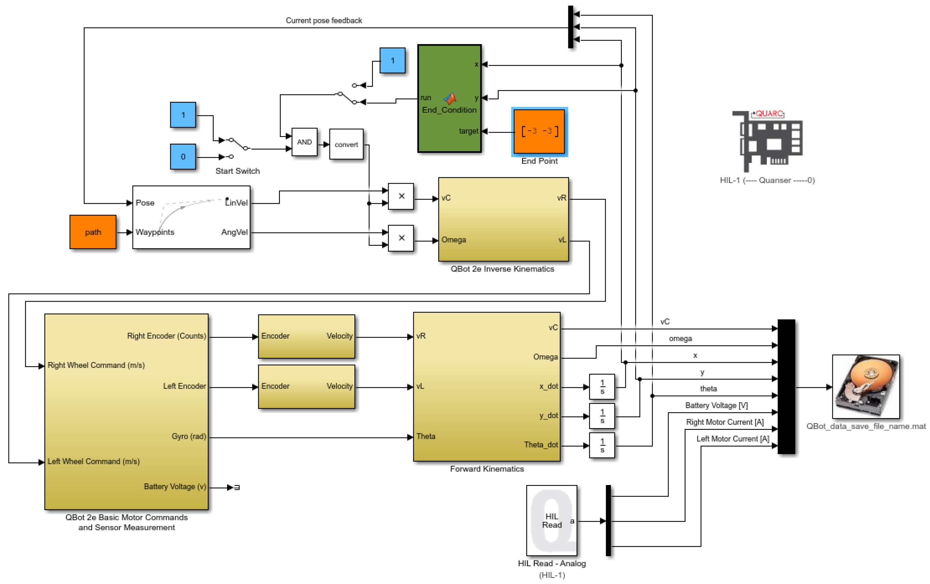
In turn, the PurePursuitCommander.slx model responsible for controlling the mobile robot was launched in the Linux environment on the Raspberry Pi target. The diagram of the model is presented in Figure 2.
The model presented in Figure 2 includes a built-in Pure Pursuit algorithm, to which data about the pose are provided, as well as a path set in the form of a matrix of waypoints. Parameters defined in Table 1 are also introduced into the model when conducting tests. These data are processed in the control algorithm block, the results are returned in the form of linear and angular velocity values of the robot at a given moment. They go to the inverse kinematics model (QBot 2e Inverse Kinematic), where they are processed into the speed values of the right and left wheels of the robot. These signals, in turn, go to the robot control block. At the same time, using this block, information from the robot’s wheel encoders is collected and converted into speeds and information from the gyroscope mounted on the robot, thanks to which data on the current position of the robot and its orientation in space are obtained. Based on the data from the sensors, using the Forward Kinematics block, values related to the state and position of the robot (angular and linear velocities, the robot pose) are obtained. The pose of the robot is passed to the Pure Pursuit algorithm block. In addition, the voltage of the robot’s battery and the current flowing through the motors driving the robot’s wheels are read. The model enables real-time recording of the robot’s operating parameters (battery voltage level, current flowing through the robot’s drive motors, angular velocity, linear velocity) and its pose (i.e., x, y and θ as an angle of the mobile platform) derived from the gyroscope readings. The results of simulations are presented in the further part of the article.

2.3. Research Methodology

Experimental research was carried out in the work, the purpose of which was to determine the value of the author’s criterion minimizing energy consumption at various values of the control algorithm parameters, such as look ahead distance, desired linear velocity and maximum angular rate. For this reason, it was necessary to carry out HIL hardware simulations of the robot’s drive for different values of the parameters of the steering algorithm, implemented using a given path. The pure pursuit algorithm was used to track the desired paths. The investigations were conducted in the following stages:
  • Determination of paths in the form of waypoints’ coordinates using the path planning module.
  • Feed the pure pursuit controller with input.
  • Conducting HIL (hardware in the loop) simulation tests.
  • Performing a comprehensive analysis of the robot’s journeys with the given initial parameters.
In the first stage, two paths were determined. One was an open path. In this case, the task of the wheeled robot was to move from the starting point to the endpoint along a given path. The second route was built in such a way that the start and end points coincided. The given paths are shown with a red line in the graphs illustrating specific results later in the article. A module supporting path planning was used to determine the paths. The task of the module was to create a table of coordinates of waypoints. The start point, end point and obstacle system have been defined in the workspace. The A* algorithm was used to plan the path of the mobile robot [47,48]. Initial conditions were individually defined for each route.
In the second stage, the table of coordinates of waypoints was passed to the pure pursuit controller. The control algorithm, in addition to indicating the parameters directly related to the construction of a specific wheeled robot, also requires three additional parameters: the linear speed of the robot, the maximum angular rate of the robot and the look ahead distance value, which determines the distance between the robot and the next point to which the robot is moving along a track defined by a set of waypoints. The look ahead distance parameter can be interpreted as the inverse of the gain of the proportional controller reproducing the given motion trajectory. The point determined by the look-ahead distance parameter is taken into account when determining the angular velocity of the robot at the current location. At this stage, the values of the parameters for which the experimental tests were carried out were also determined. Input parameter combinations (same for both paths) are shown in Table 1.
In the third stage, HIL (hardware in the loop) simulation tests were carried out, the same for both paths. They consisted in driving the mobile robot from the starting point of the route, along the desired path, to the endpoint. The end point was represented by a circle with a radius of 10 cm centered on the last waypoint of the path. The robot’s entry into the area defined in this way was considered a complete run—the robot stopped. For each of the tested paths, twenty-seven runs were made, taking into account all combinations of input parameters presented in Table 1. During the experiments, combinations of control algorithm parameters were observed, which caused the robot to behave inappropriately, such as unexpectedly stopping, leaving the working area, or driving into an obstacle. In such a situation, the experiment was interrupted and these trips were not taken into account during the analysis of the results. If the ride, for a specific set of input data delivered to the controller, was successful, i.e., reaching the endpoint of the path, then the robot’s motion parameters (specified above) were recorded for use in the next stage.
The last, fourth stage consisted in conducting a comprehensive analysis of all travels. At this stage, the data recorded during the HIL simulation were analyzed. This stage was divided into two parts. In the first part, based on the measurement data, the values of the parameters included in the evaluation criterion, i.e., the energy used to cover the path, travel time and the path matching accuracy were determined. The first parameter, i.e., the energy consumed during the journey, was calculated as the product of the robot’s battery voltage and the current flowing through the wheel drive over time.
P l = U A · I l , P r = U A I r ,
where P l —power measured for the left motor, P r —power measured for the right motor, U A —battery voltage, I l —current measured for the left motor, I r —current measured for the right motor.
The energy was calculated for the left and right wheels separately and finally added together. The values determined in this way in subsequent time intervals were summed up. In this way, the total value of energy consumed by the robot during the route was obtained
E T = E L + E R = i = 1 n P l i + i = 1 n P r i n ,
where E T —total energy consumed for travel of the given path, E L —energy consumed by the left motor, E R —energy consumed by the right motor.
The second parameter was the robot’s travel time. This value was defined as the difference between the start time and end time of the robot’s travel. The starting time is the beginning of the movement (the value of the recorded linear velocity greater than zero) from the starting point where the mobile robot was placed each time before the start of the simulation. The end time is understood as reaching the end area defined as a circle with a radius of 10 cm centered on the last waypoint.
The last parameter of the criterion, i.e., the path matching accuracy was determined using the Hausdorff measure. The pose of the robot was recorded every 0.01 s. Due to the big size of the data, the values were aggregated to 0.1 s intervals. The number of robot positioning points varied depending on the choice of path parameters. The number of points has been unified. A fixed number of points was established to calculate the Hausdorff measure. Its value was equal to the number of points forming the shortest path. In the case of paths with a greater number of points, they have been determined in proportion to the length of the path.
The selected evaluation parameters differed by orders of magnitude. The authors wanted each of the parameters to have an equal impact on the final assessment of the selection of input parameters. For this reason, it was decided to normalize the parameters in accordance with the formula below:
E T n o r m = E T m a x ( E T ) m i n ( E T ) + m i n ( E T ) ,
T t t n o r m = T t t m a x ( T t t ) m i n ( T t t ) + m i n ( T t t ) ,
H D n o r m = H D m a x ( H D ) m i n ( H D ) + m i n ( H D ) .
The maximum and minimum values of a given parameter were determined for the set obtained after the robot traveled a given path twenty-seven times—so as to record arrivals with all combinations of input parameters. After this operation, each parameter changes in the range from 0 to 1. In the second part of the stage, the following cost function was defined
f ( E T n o r m , T t t n o r m , H D n o r m ) = ( E T n o r m ) 2 + ( T t t n o r m ) 2 + ( T t t n o r m ) 2 ,
where E T n o r m = E T n o r m ( v , ω , L d ) —total energy consumed for traveling the given path, normalized with Formula (5), T t t n o r m = T t t n o r m ( v , ω , L d ) —total time of travel the given path normalized with Formula (6), H D n o r m = H D n o r m ( v , ω , L d ) —Hausdorff’s measure normalized with Formula (7), v—desired linear velocity, ω —maximum angular rate, L d —look ahaed distance.
For each simulation, the values of the parameters E T n o r m , T t t n o r m , H D n o r m , and then the values of the cost Function (8) were determined. Subsequently, for each path, the cost Function (8) was minimized regarding the E T n o r m , T t t n o r m and H D n o r m parameter.

3. Results

3.1. Results for Track 1

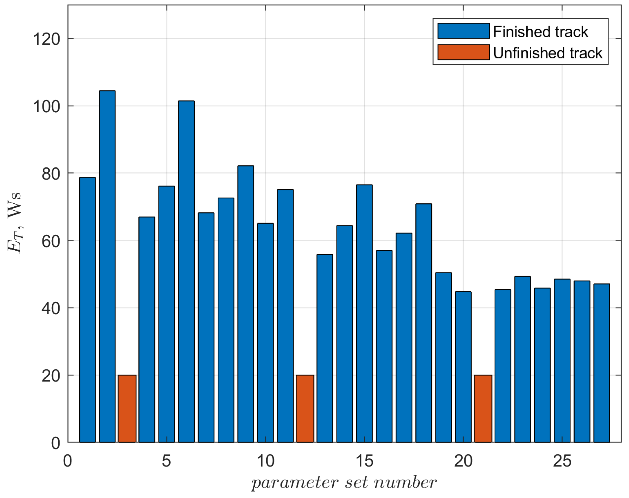
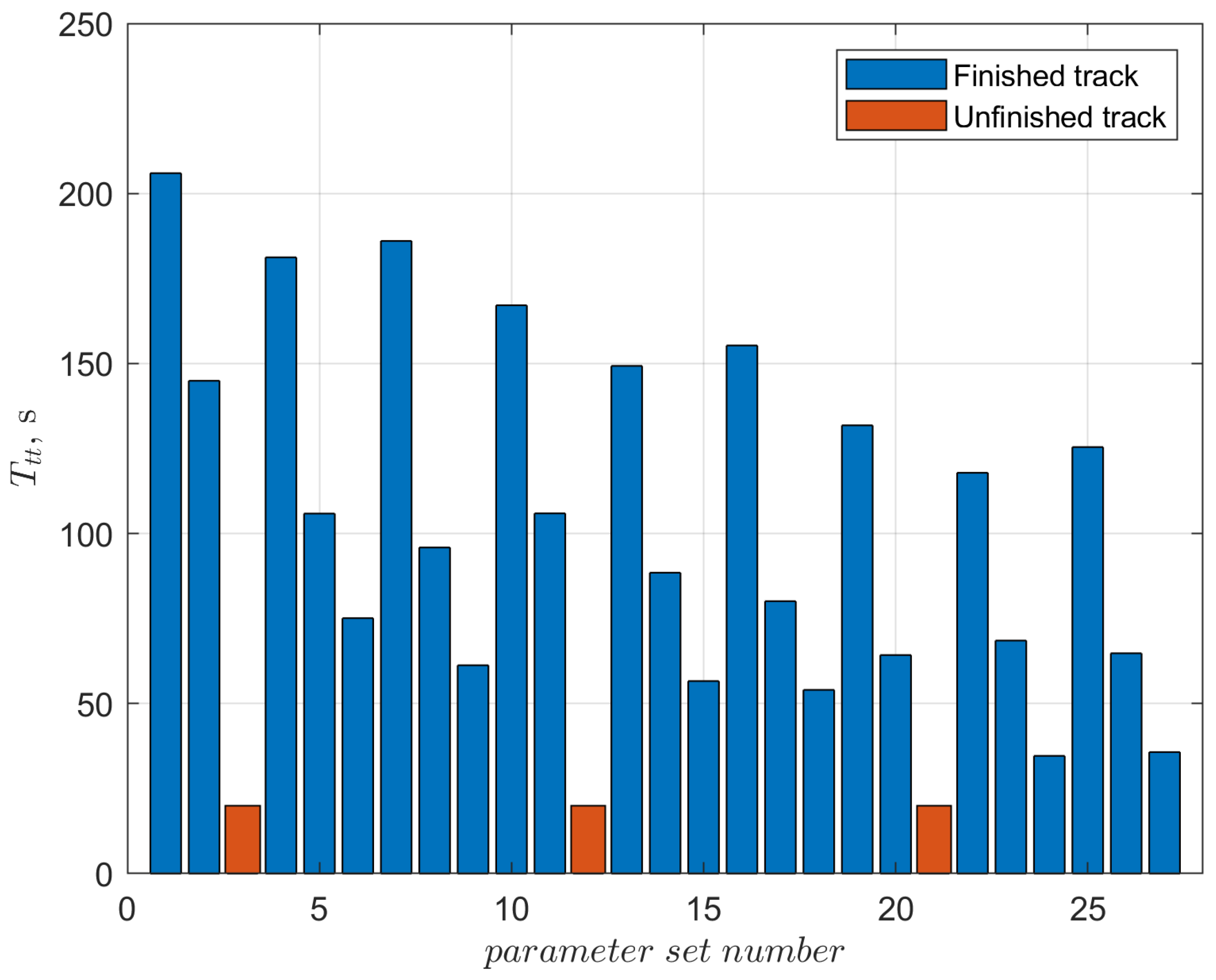
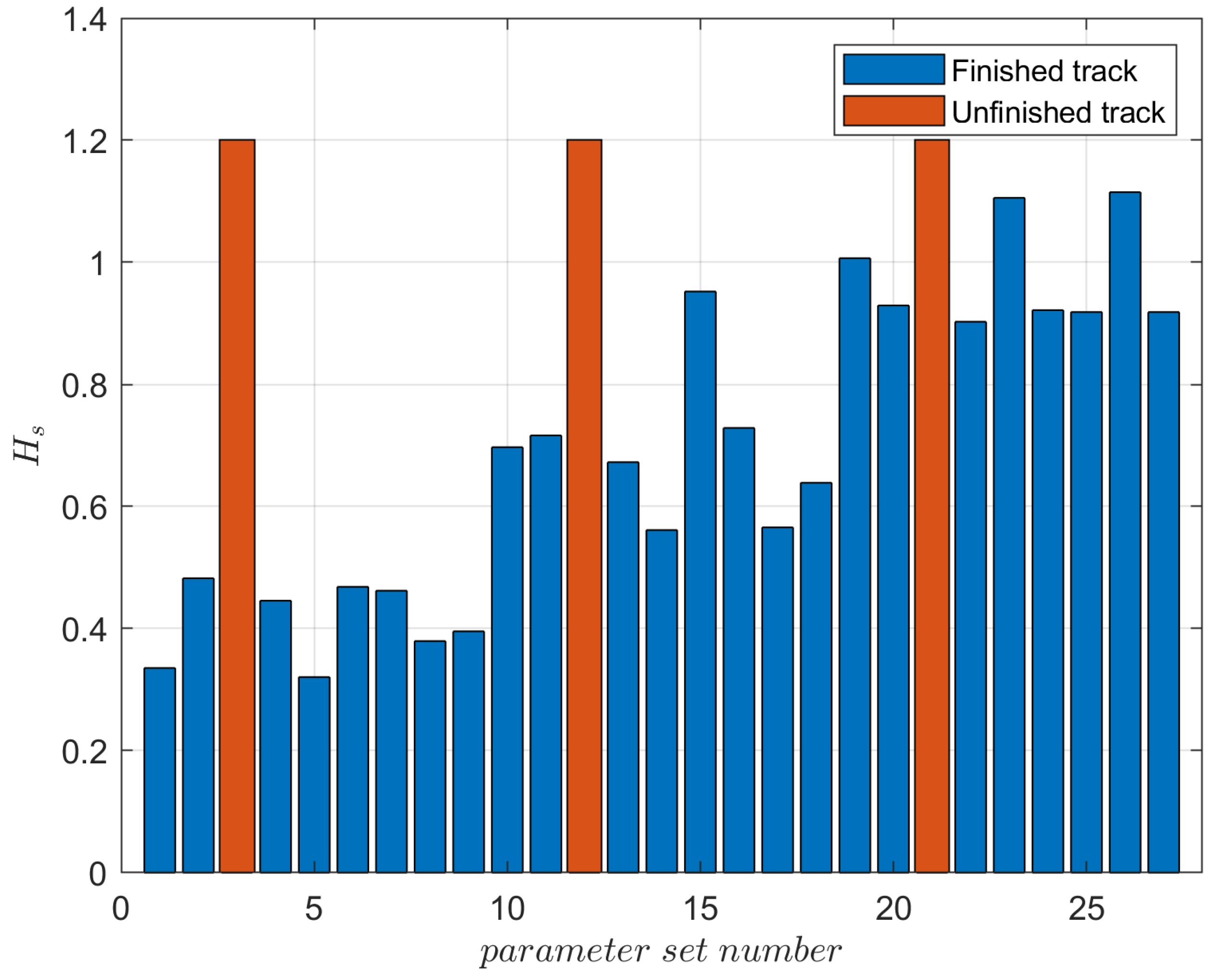
In this paper, the simulation studies involving completing the given paths by a wheeled robot controlled by the pure pursuit controller with predetermined parameters were carried out. The values of individual parameters, i.e., linear velocity, maximum angular velocity and look ahead distance, are presented in the form of variants collected in Table 1. It should be noted that in the case of path 1, three variants with index numbers: 3, 12 and 21 were excluded from the further analysis. In the case of setting parameter values according to these variants, the robot did not perform the task correctly, i.e., it did not reach the endpoint of the given path. Parameter values of excluded variants are presented in Table 2. Excluded variants are represented by red bars in Figure 3, Figure 4 and Figure 5.
It was observed that in the case of two variants, i.e., the second and fourth, the energy consumption exceeds 100 Ws. These values differ significantly from the others. On the other hand, the minimum value of energy consumption falls on variant 20. Additionally, it should be noted that in the case of variants 22–27, the values of energy used to complete the path are slightly higher than the minimum value. Analyzing the parameter values of individual variants, it is visible that the value of energy necessary to complete the path decreases with the increase in the look-ahead distance parameter. Some influence of linear velocity changes is also noticeable. Increasing the value of this parameter increases the energy consumed during traveling the entire path. These observations are carried out while maintaining constant values of the other input parameters.
The time needed to complete the path is the largest in the case of the first variant, (i.e., exceeds 200 s). On the other hand, the robot completes the path the fastest using the 24th set of parameters, it took a little more time to complete the path using the 27th variant (see: Table 1). In Figure 4, it seems to be obvious, that a strong impact of the linear speed value on the travel time. The higher the speed, the faster the robot completed the path (while maintaining constant values of other parameters). To a lesser extent, the travel time is affected by the look-ahead distance. Increasing it shortens the travel time. The maximum angular rate affects the travel time to the smallest extent.
The smaller the value of the Hausdorff measure, the more accurately the given path is mapped. The smallest value occurs in the case of the fifth variant and amounts to 0.3205. A slightly worse mapping was obtained using the first variant (0.3354). Variants 23 and 26 are on the opposite extreme. In this case, we are dealing with the two worst mappings of the given path. The values of the Hausdorff measure are 1.1056 and 1.1149, respectively. Figure 5 shows a clear trend of increasing the value of the Hausdorff measure with the increase in the value of the look-ahead distance parameter. We deal with intermediate variants when the look-ahead distance value is 1.0 m.
Since the authors wanted to maintain an equal impact of individual component functions on the final value of the cost function, standardization of component functions was applied. As a result, the cost function can change values in the range from 0 to 3. The zero value of the function means that all component parameters have reached their minimum values, i.e., the lowest energy consumption, the shortest travel time and the best fit in the set of analyzed variants.
The smallest value of the cost function is 0.8735 and was obtained for 17th set of parameters (see: Table 1). The optimal values of individual parameters are: v = 0.2 m/s, ω = 0.9 rad/s, L d = 1.0 m. The confirmation of the values of these parameters can be found in Figure 6, Figure 7 and Figure 8. The highest value of the cost function is for the second variant and is equal to 1.2970. The next largest one is represented by the first variant and equals 1.2878.
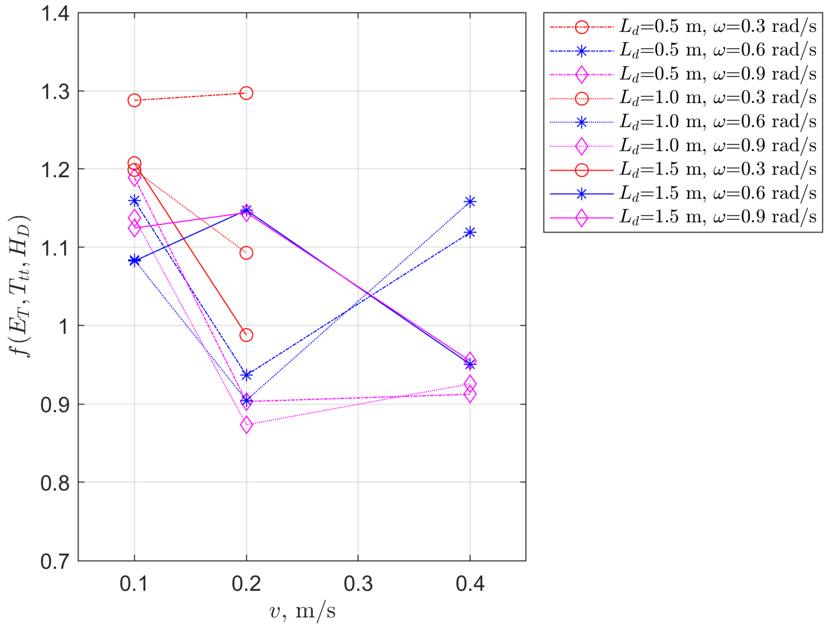
The influence of the linear speed on the value of the cost function is shown in Figure 6. It can be stated that in the case of an intermediate value ( 0.2 m/s) the cost function values reach local minima in four cases and local maxima in two. In three cases, we cannot determine it because we do not have complete data. Local maxima occur for L D = 1.5 m, and local minima when look ahead distance is less than 1.5 m.
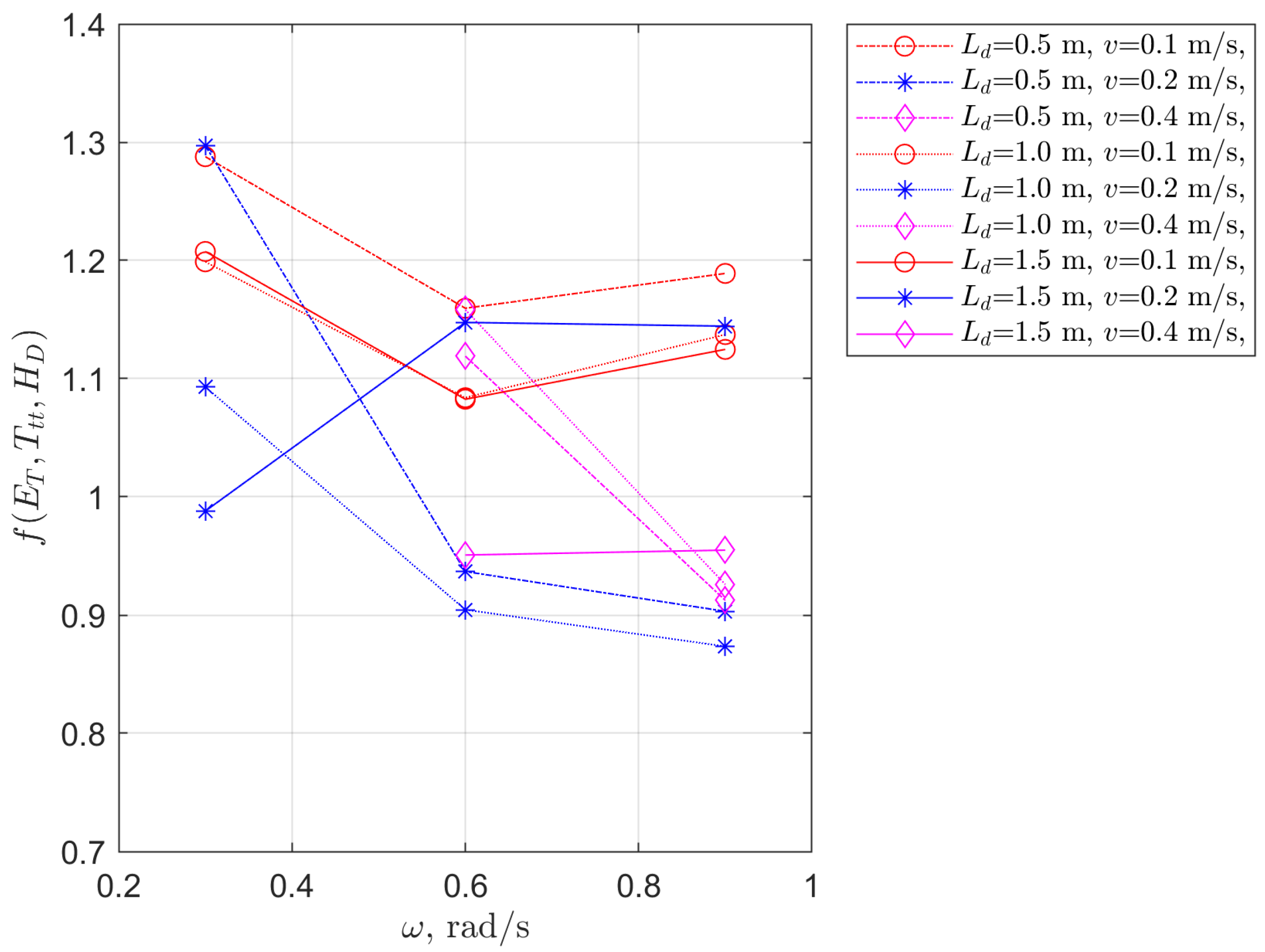
The presence of local minima can also be observed in Figure 7. However, it only occurs for variants marked with red, i.e., for a linear velocity of 0.1 m/s. In other cases, it is difficult to indicate clear trends. It can also be concluded that (except for one case) higher values of the cost function appear in the case of the maximum angular rate equal to 0.3 m/s.
It is difficult to clearly determine the impact of the look-ahead distance parameter on the value of the cost function presented in Figure 8. Depending on the selection of other parameters, one can find increasing and decreasing trends, as well as local maxima and minima.
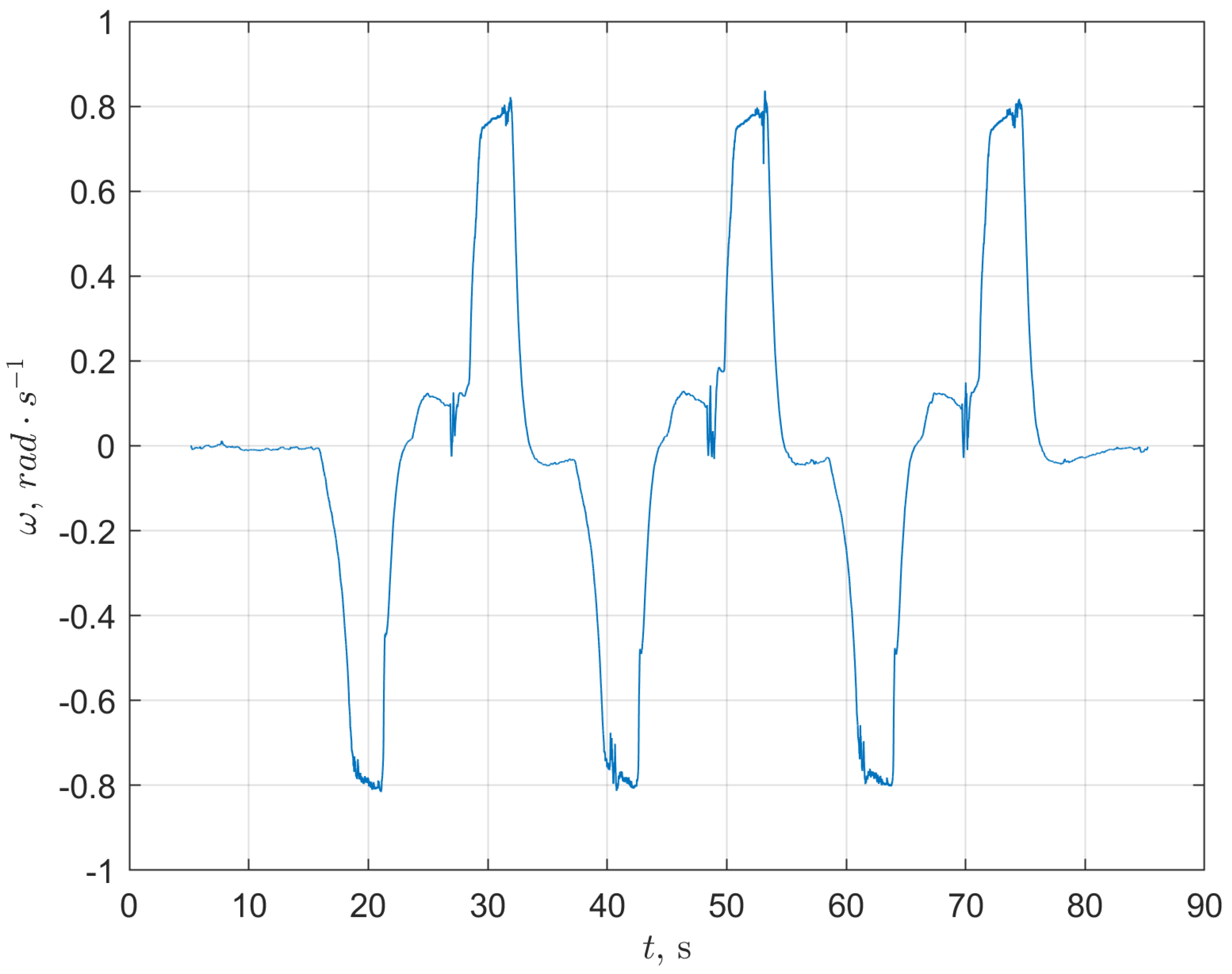
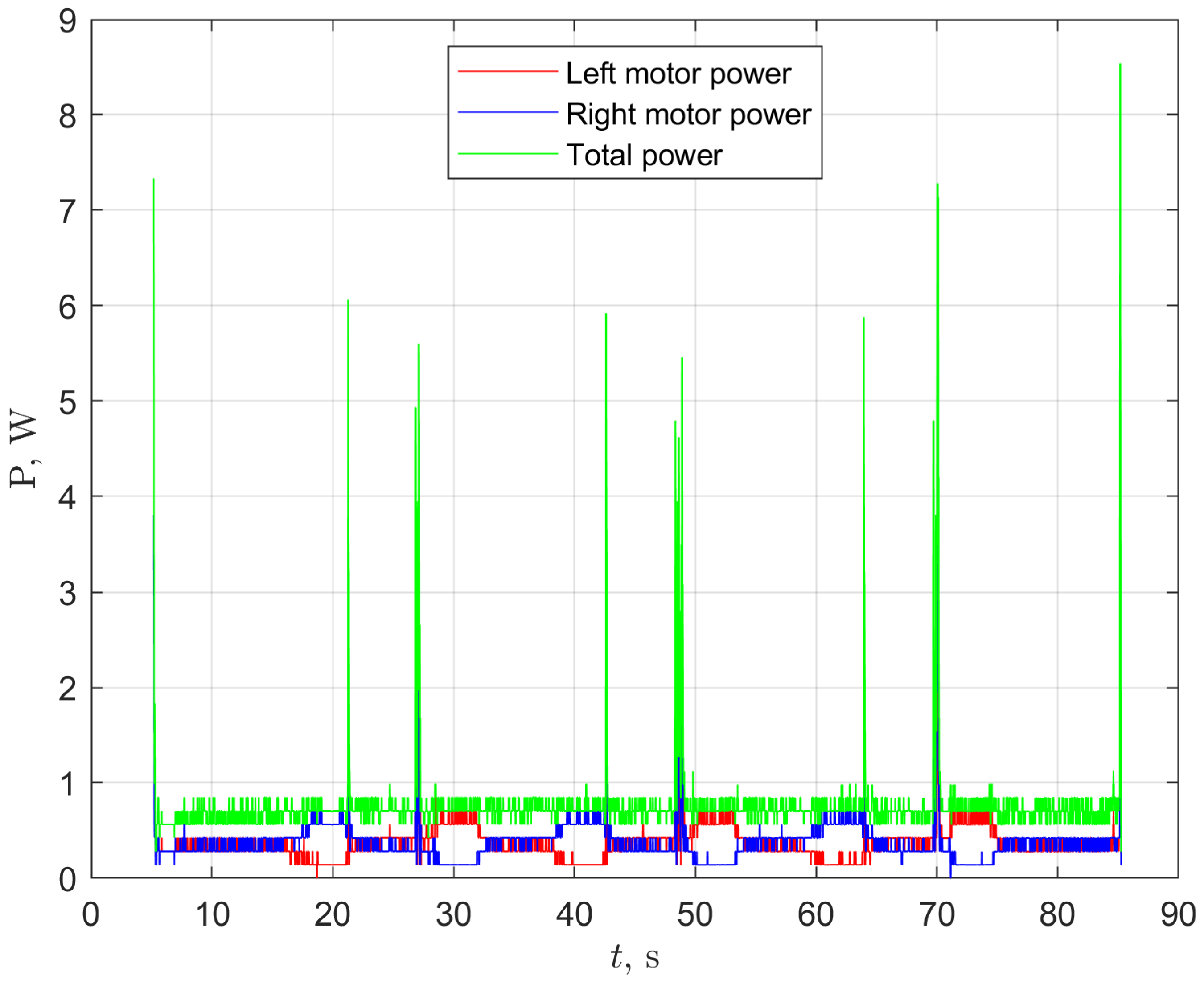
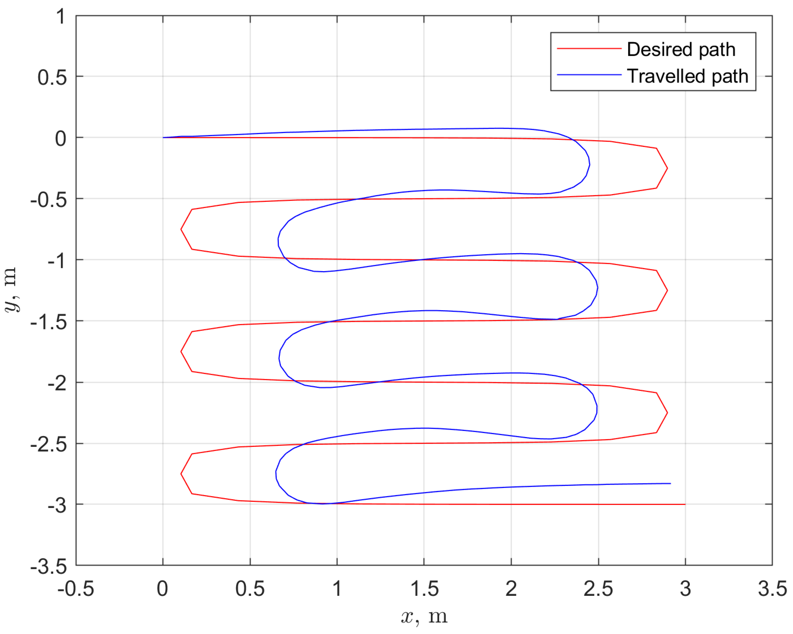
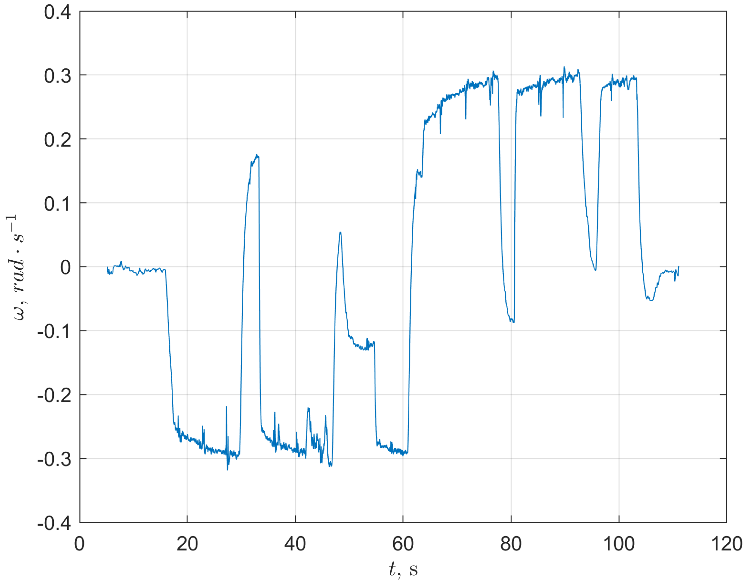
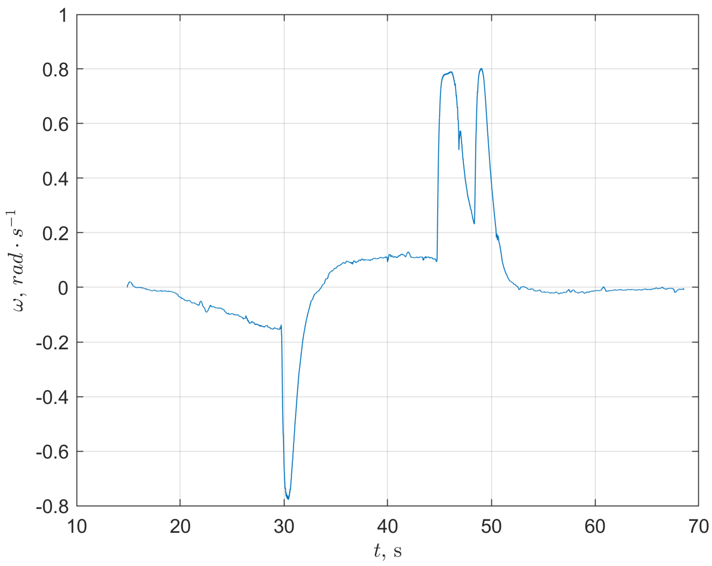
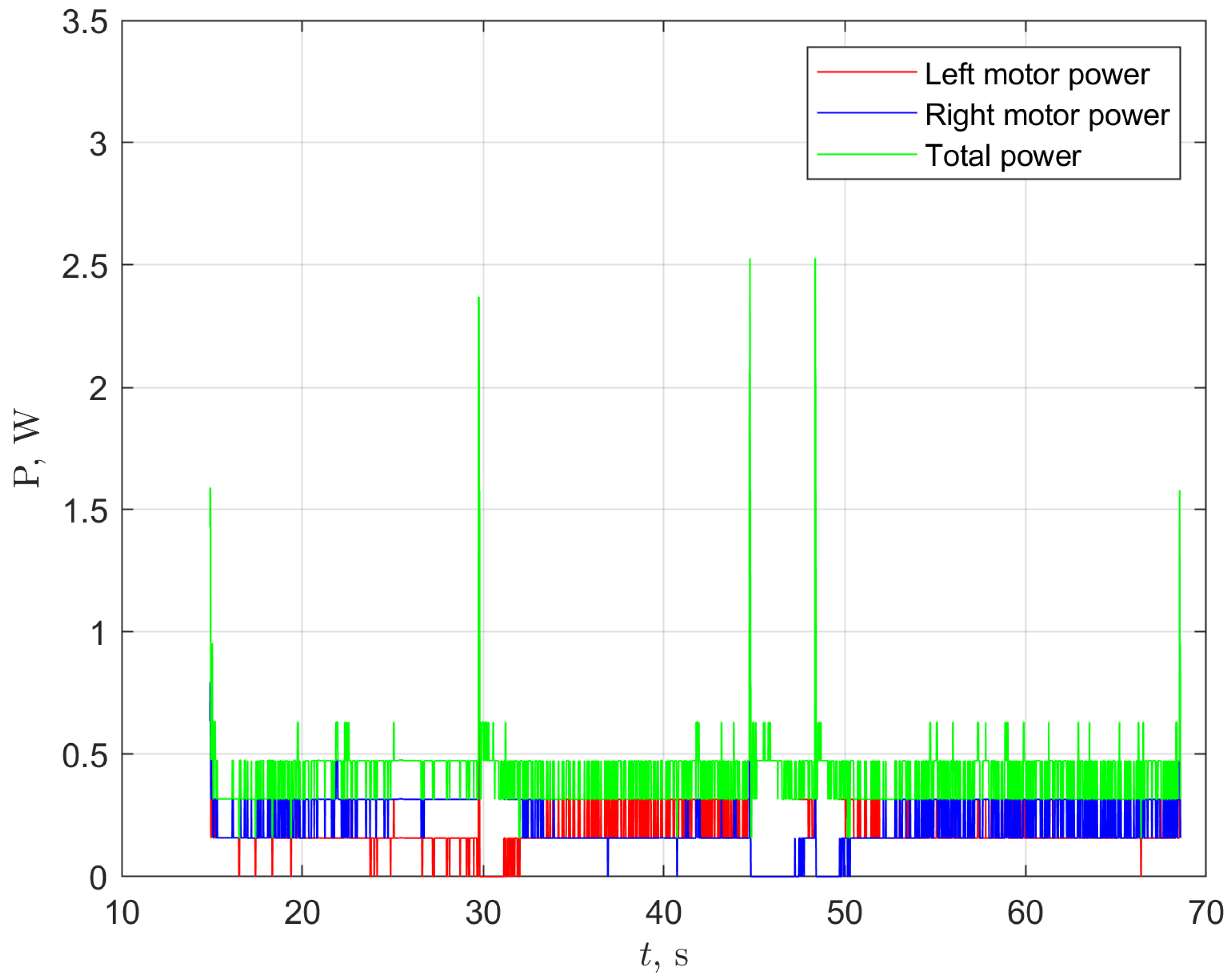
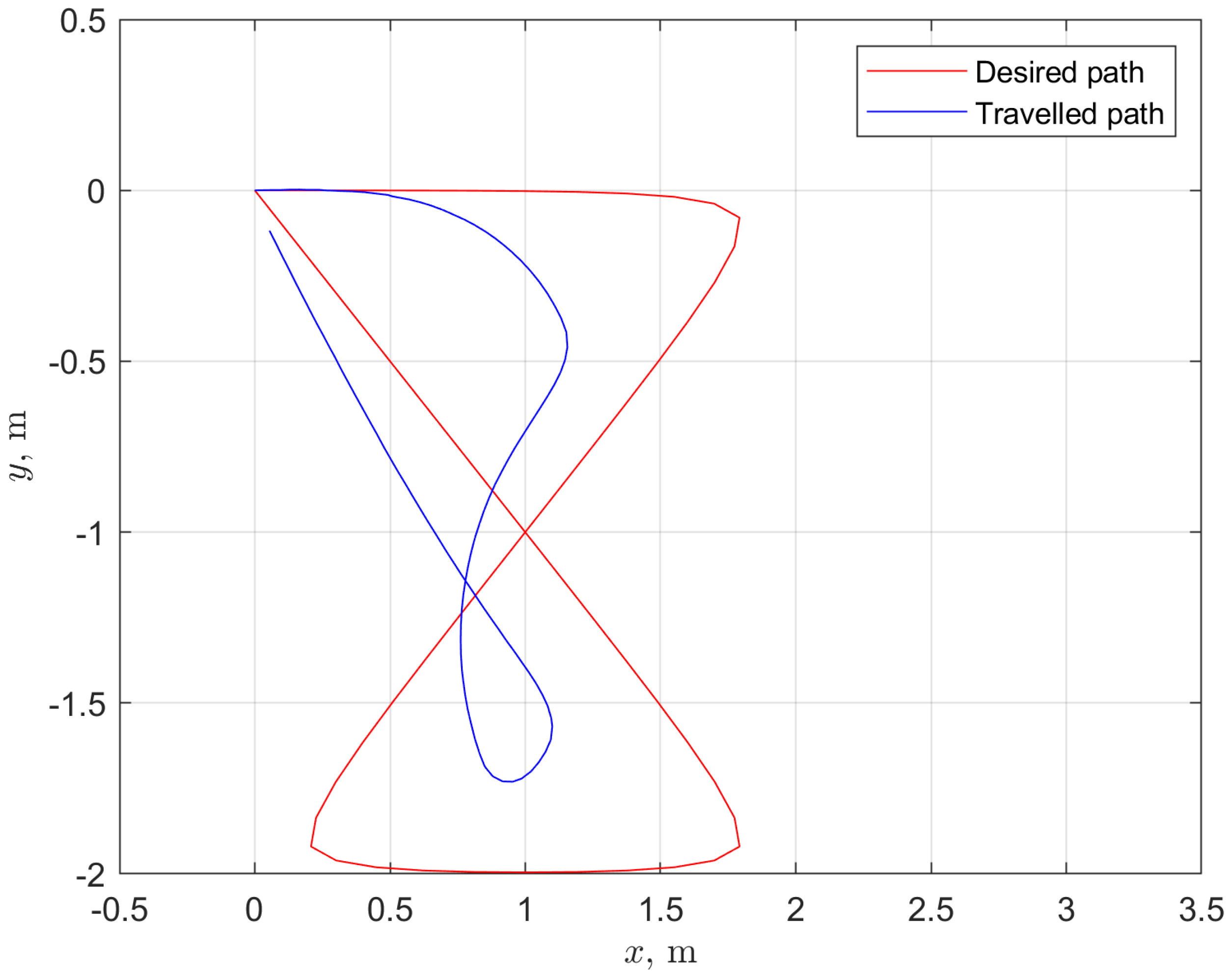
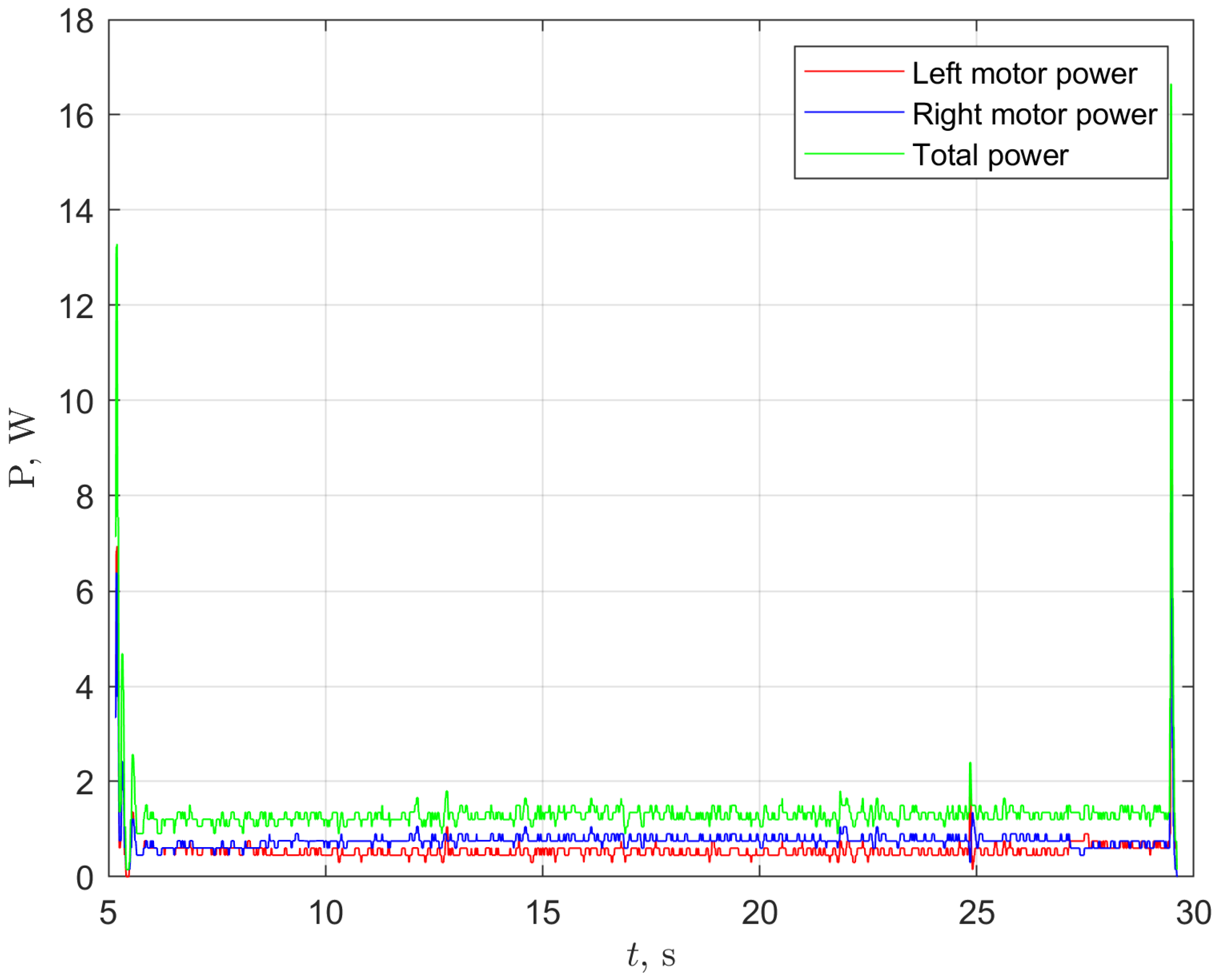
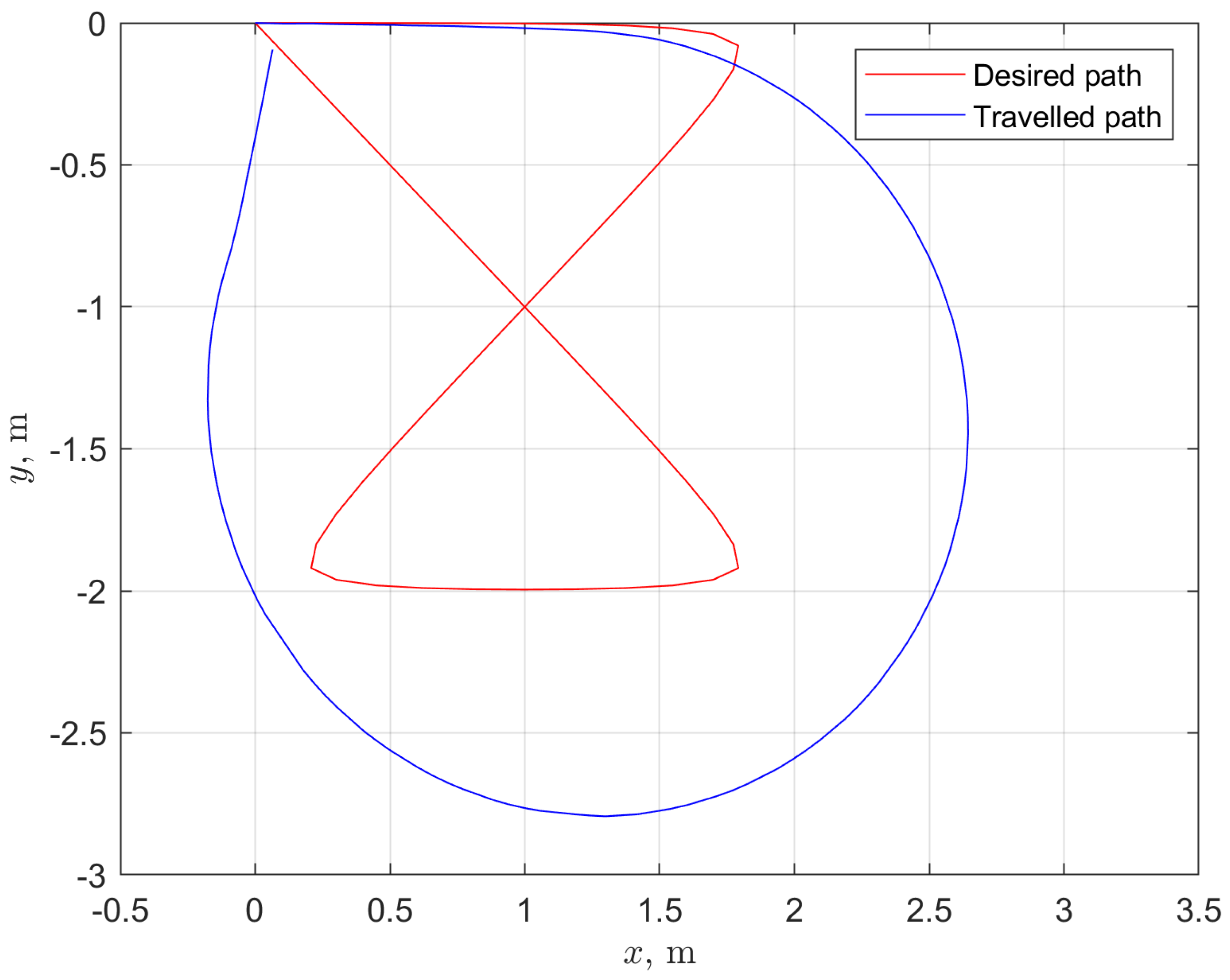
Figure 9, Figure 10 and Figure 11 show selected parameters of the travel for which the cost function reached the lowest value. Figure 9 and Figure 10 show, respectively, the variability of angular rate and power during the robot’s traversing the path. Figure 11 shows the given (reference) path and the path actually traveled by the robot, for which the input parameters were established in accordance with 17th variant (see: Table 1).
In Figure 12, Figure 13 and Figure 14, it was shown a case where the cost function reached the middle value of 1.0930. This situation occurred for the 11th parameter set. In this case, the input parameter values are v = 0.2 m/s, ω = 0.3 rad/s and L d = 1.0 m. Comparing Figure 11 and Figure 14, we can see a better match of the path for the 17th simulation variant. In Figure 12, it is shown a greater irregularity in the variance of the angular rate compared to the change in the angular rate for the best case.
In the worst case, the value of the cost function was 1.2970. Figure 15 and Figure 16 show selected travel parameters that change over time. Figure 17 shows the path-matching accuracy. This case occurred for the parameter set number 2, i.e., v = 0.2 m/s, ω = 0.3 rad/s, L d = 0.5 m. In this case, the accuracy of the path mapping was the best, which is also confirmed in Figure 5. However, due to the relatively long travel time and the largest amount of energy consumed, the final value of the cost function turned out to be the largest in relation to the other HIL simulation variants.
In the work, the values of the standard deviation of individual, normalized components of the cost functions were also determined. For the first given path, they were: σ E c = 0.1608 , σ T t t = 0.2414 and σ H D = 0.2267 . These values indicate less variation in the energy-related component. The value of the standard deviation of the cost function was σ f = 0.1282 .

3.2. Results for Track 2

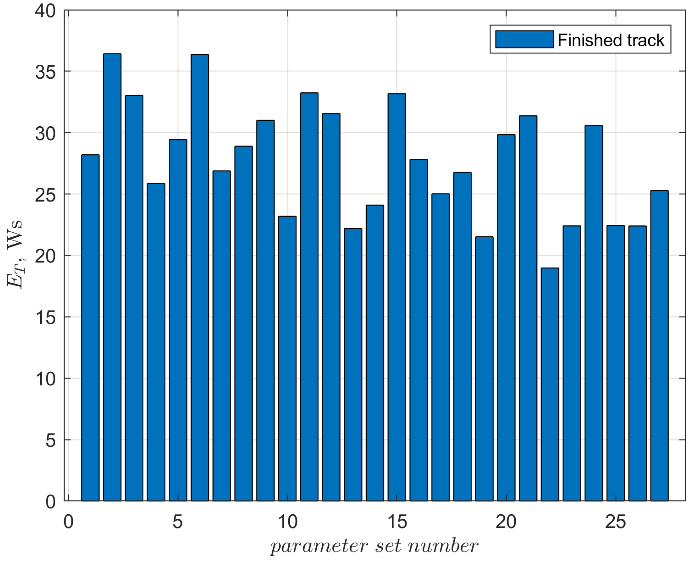
In the case of the given track 2, the set of parameter variants presented in Table 1 was also used. All runs, with the set parameter values according to the variant number were successful. The robot has reached the endpoint of the path each time. The value of energy used to complete path 2, in most cases, ranges from 20 Ws to 35 Ws. In one case, when it is also the lowest value, it drops below 20 Ws. In two cases, for variants 2 and 6, it exceeds 35 Ws. This information is shown in Figure 18. The travel time is strongly dependent on the desired linear speed. This relationship is inversely proportional. It is also possible to notice the influence of the maximum angular rate on the travel time of the mobile robot. As in the case of linear velocity, also in the case of the maximum angular rate, the travel time decreases with the increase in value of the maximum angular rate. These relationships are illustrated in Figure 19.
Analyzing Figure 20, we can see three almost equal values of the Hausdorff measure. They represent 3rd, 12th and 21st simulation variant. These variants (parameter sets) differ significantly from the others and the values indicate a large mismatch between the actually traveled path and the desired path. These variants indicate a specific combination of linear velocity and maximum angular rate. In addition, these are the same variants for which path 1 failed, the variants are presented in Table 2.
Analyzing the influence of the look-ahead distance parameter on the Hausdorff measure, it can be stated that increasing its value increases the value of the Hausdorff measure, i.e., worsens the accuracy of the path matching. Apart from the three cases mentioned above, variants 2 and 6 are also an exception. In cases of these two variants, the ratio of the maximum angular rate to the linear velocity is the smallest (after rejecting variants 3, 12 and 21).
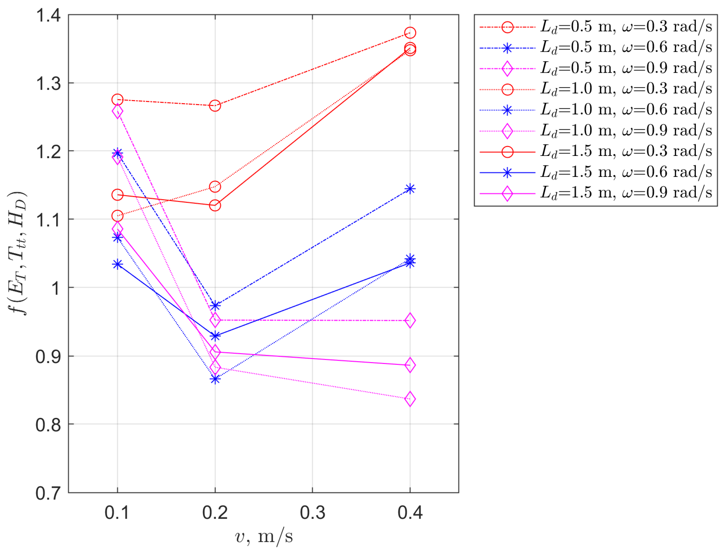
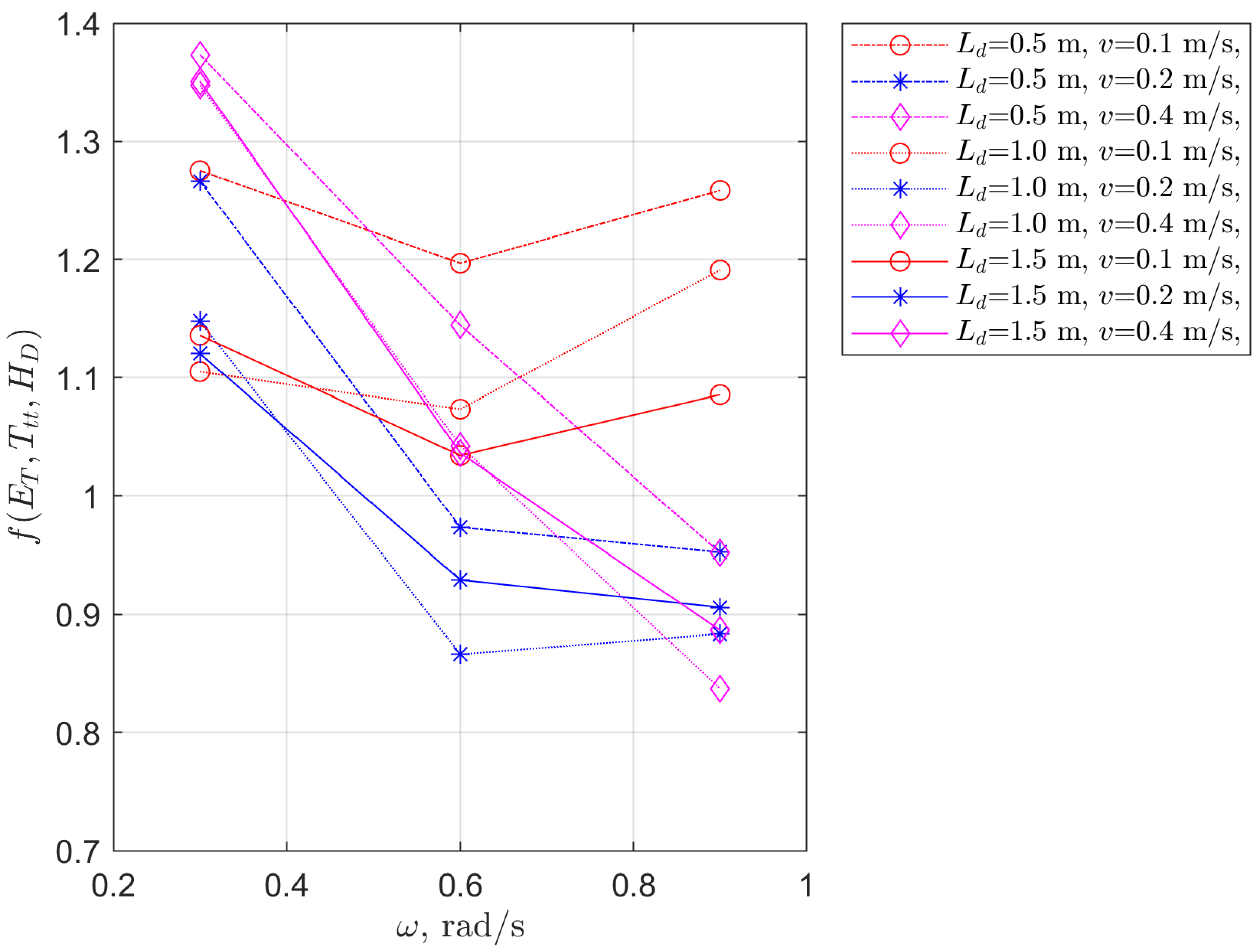
In the case of the cost function, taking into account the impact of all three components, it turned out that the best set of parameters is variant number 18. In this case, the lowest value of the cost function was obtained, amounting to 0.8369. The values of the individual input parameters are v = 0.4 m/s, ω = 0.9 rad/s and L d = 1.0 m. In turn, the largest value of the cost function was 1.3732. It was obtained for variant 3, i.e., a set of input parameters of v = 0.4 m/s, ω = 0.3 rad/s and L d = 0.5 m. These quantities can be easily identified in Figure 21, Figure 22 and Figure 23. In addition, these Figures confirm the observation visible in Figure 20 regarding three variants with values that differ from the others. In this case, there is a large influence of the value of the Hausdorff measure on the final value of the cost function. This can be seen especially in Figure 23, where the highest curve corresponds to the indicated variants. In addition, Figure 21 shows a difference between the behavior of the cost function values in individual groups marked with separate colors. The colors indicate the change in the value of the maximum angular rate. It also shows a strong dependence of the cost function value on the maximum angular rate.
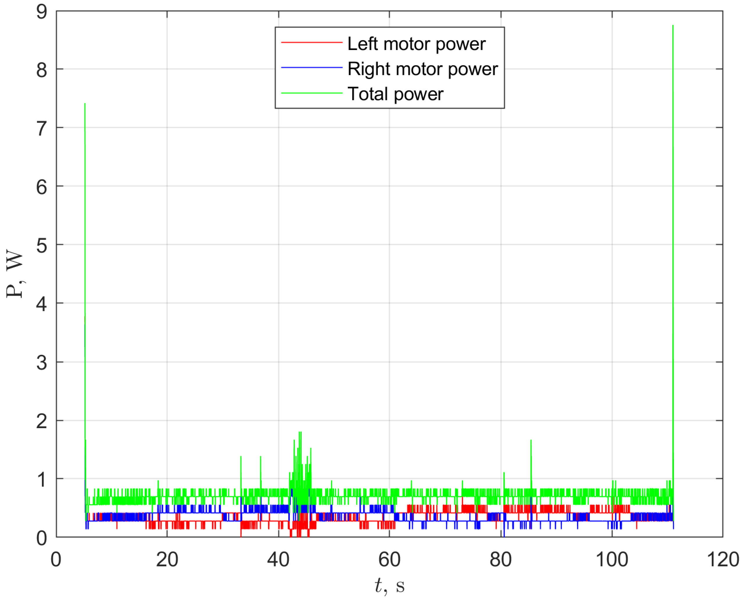
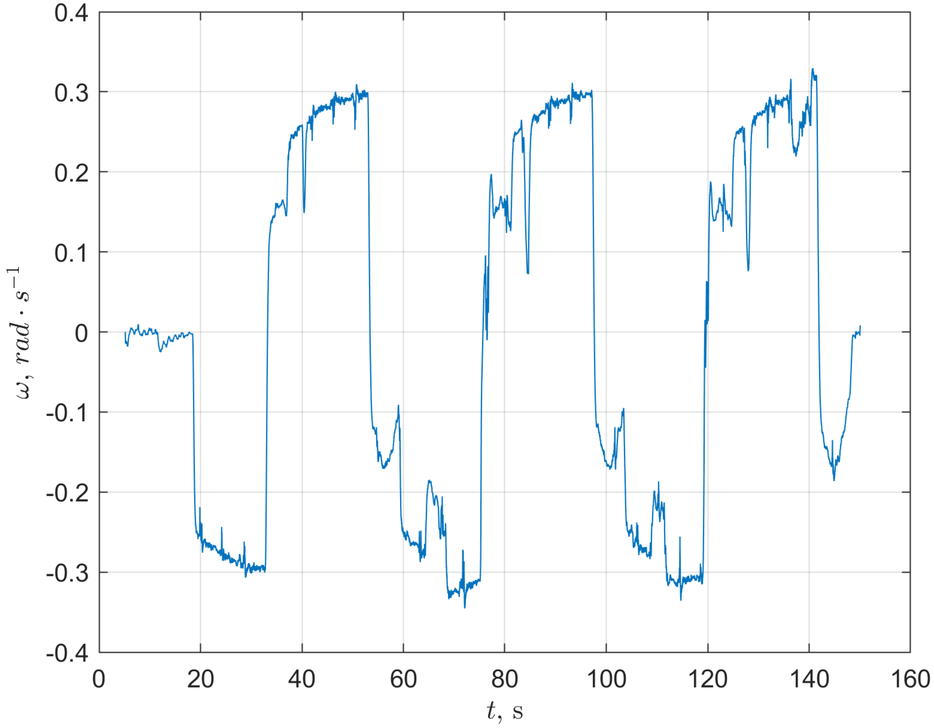
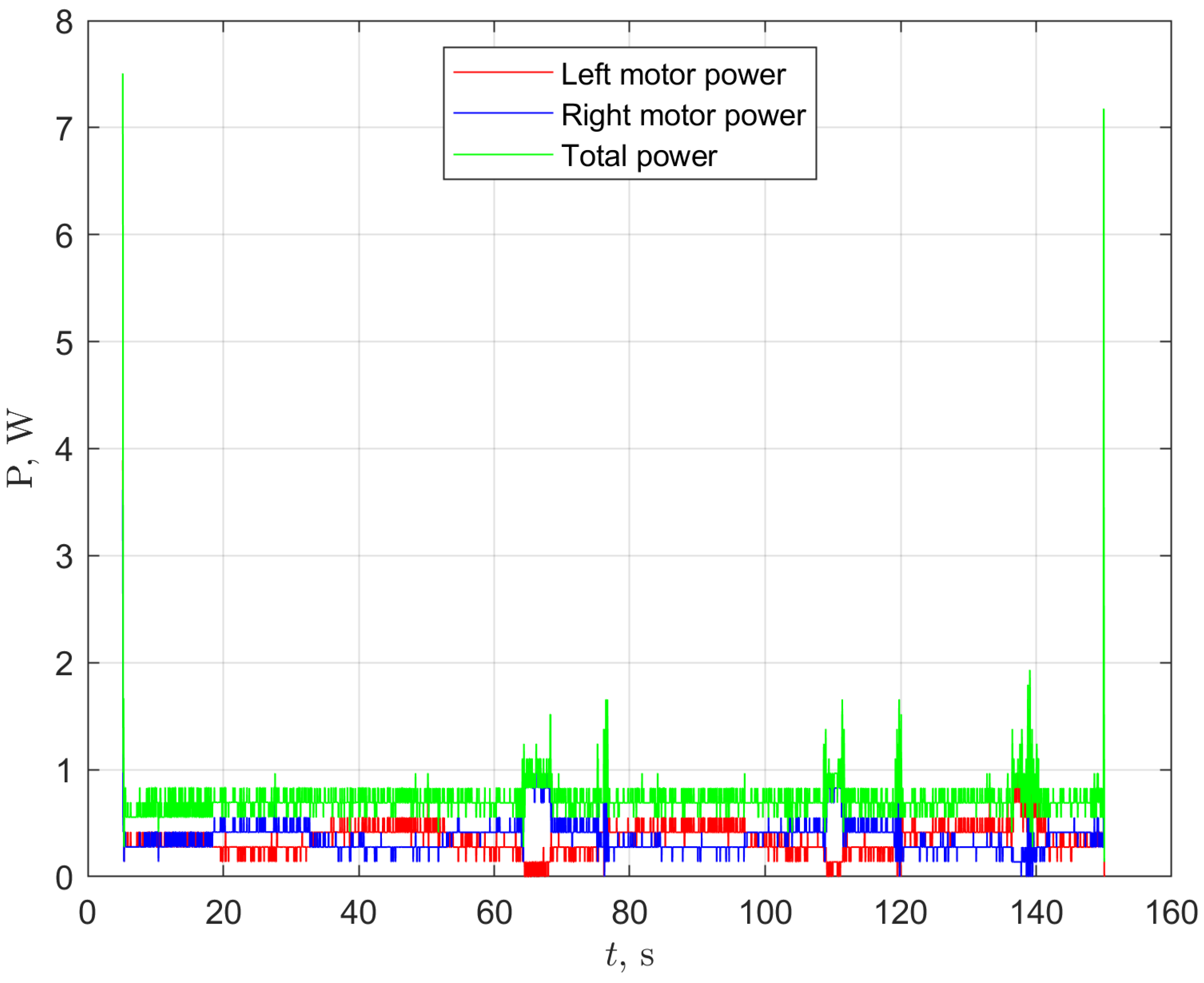
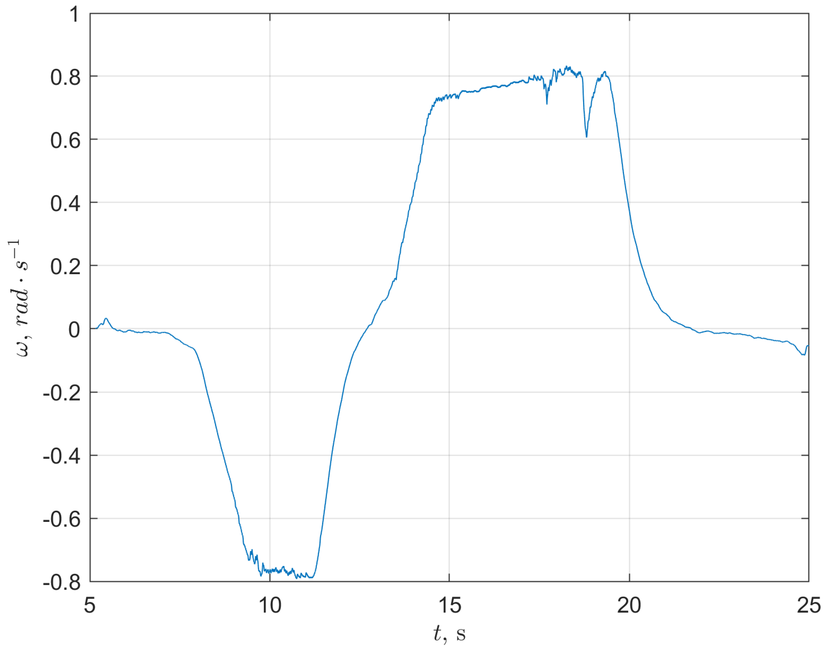
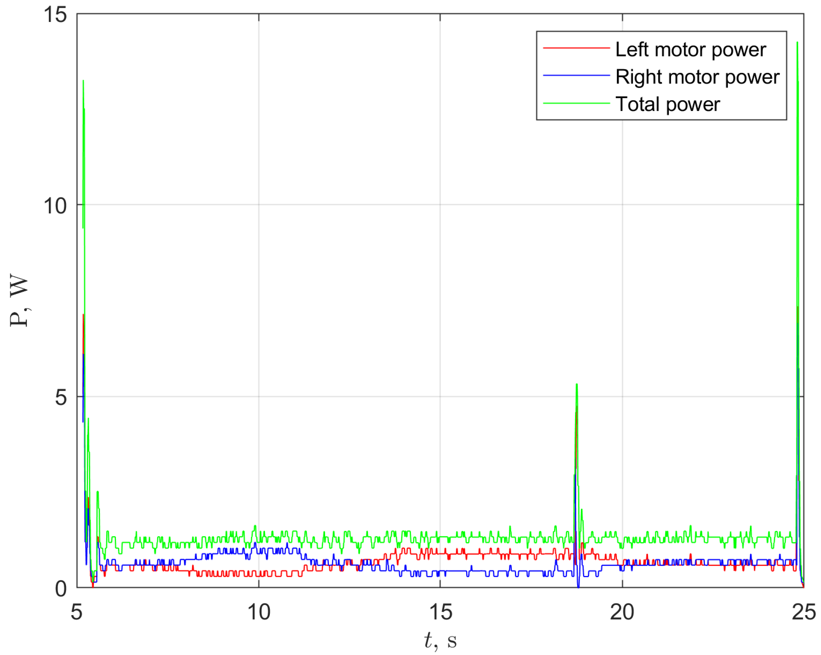
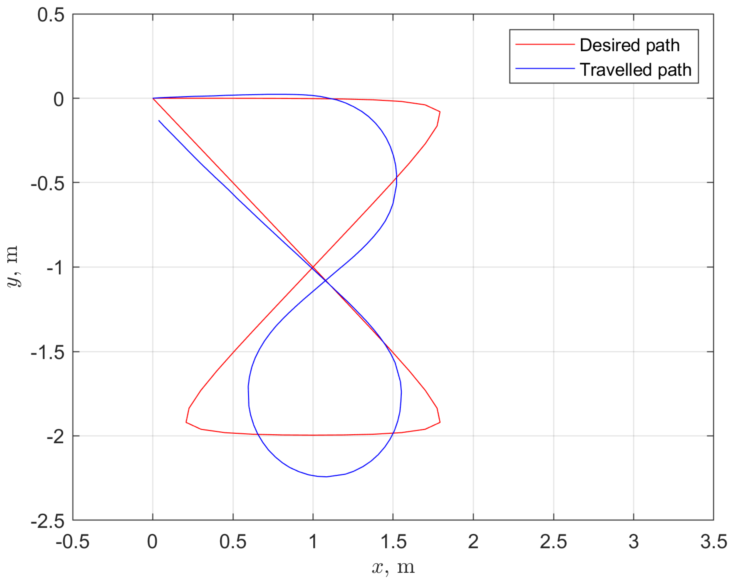
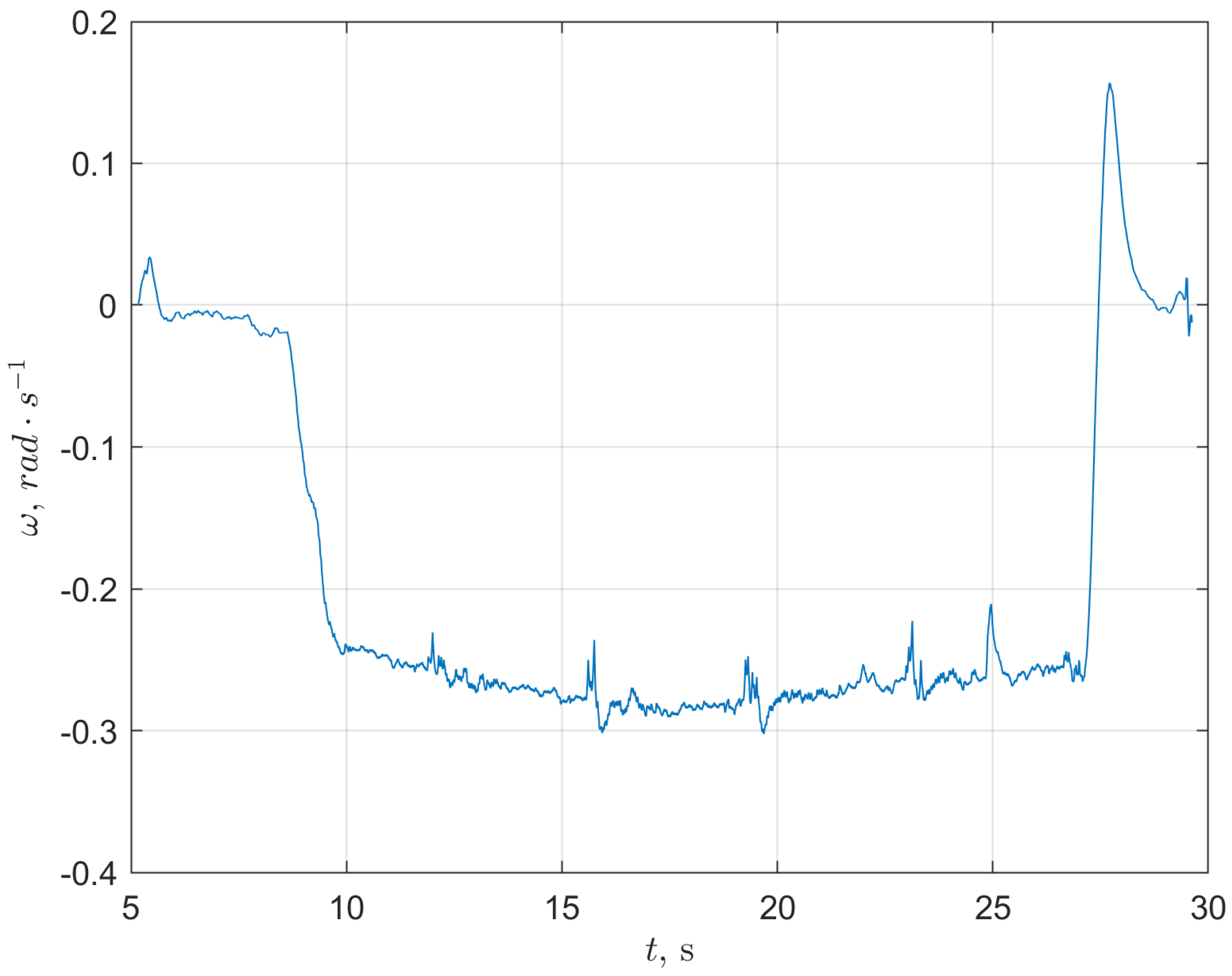
Figure 24, Figure 25 and Figure 26 show respectively the change in the angular rate, the change in the power value and the comparison of the path planned and traveled by the mobile robot for the smallest value of the cost function. In this case, there is one moment during the path in which the angular rate changed significantly. This change is also confirmed in Figure 25, where a sudden increase in power is visible. Of course, this increase is also visible at the beginning and end of the path. It is related to the starting and stopping of the mobile robot.
Detailed data related to the variant of the intermediate value of the cost function is presented in Figure 27, Figure 28 and Figure 29. In this case, the value of the cost function was 1.0858. It was achieved for variant number 25. In Figure 27, it was shown more frequent and rapid changes in the angular rate of the mobile robot in relation to the data presented in Figure 24. This is also reflected in Figure 28, where changes in angular rate are correlated with an increase in power demand. Comparing Figure 25 and Figure 28, there is a drastic difference in the demand for specific power during both travels. It results directly from the set value of the robot’s linear velocity, which is v 18 = 0.4 m/s and v 25 = 0.1 m/s, respectively. It should be noted that the total energy used to complete the path according to both variants does not differ as much as the power values would indicate. Lower unit power consumption is associated with a longer travel time of the given route by the robot.
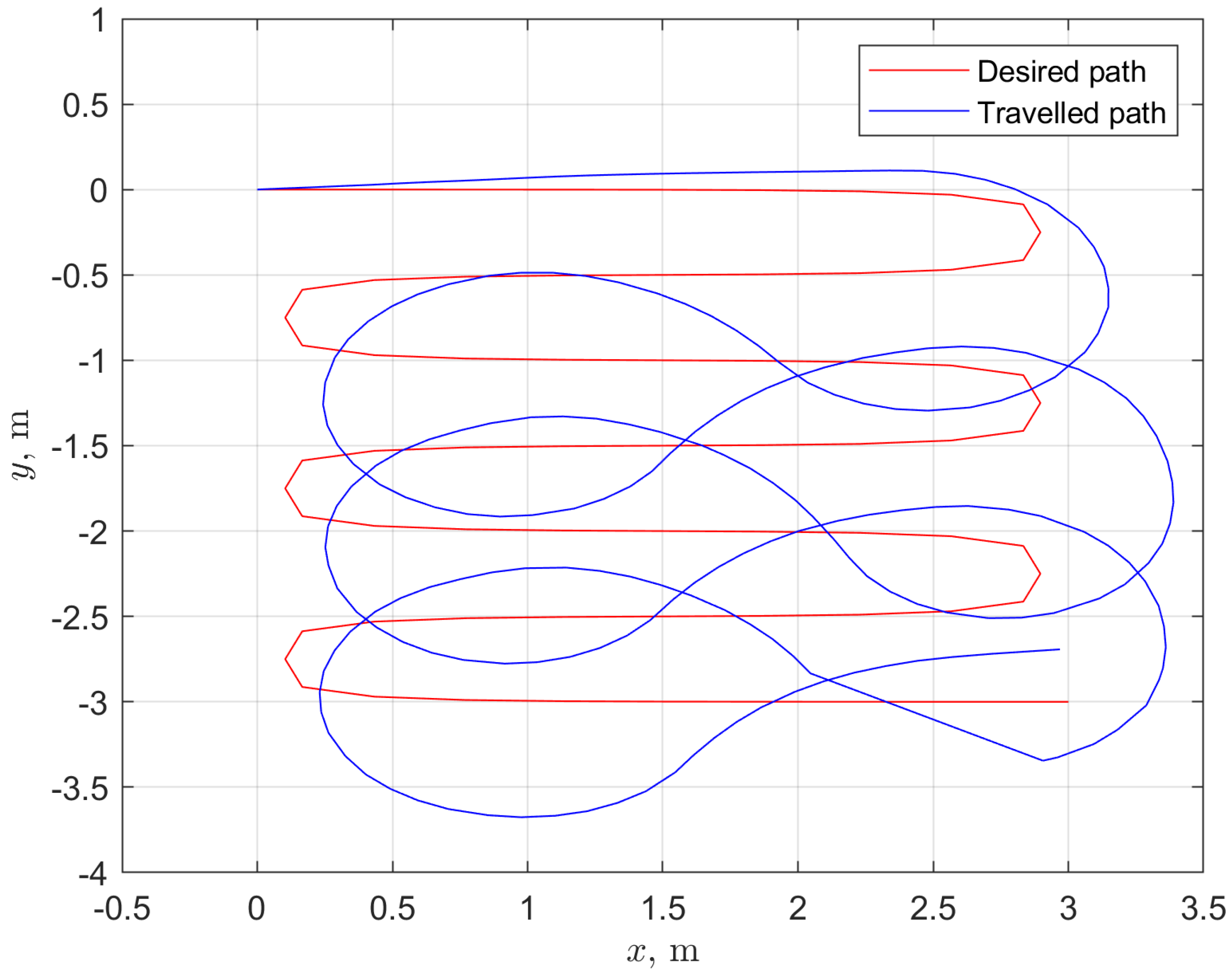
In the worst variant, i.e., variant no. 3, the cost function reached the value of 1.3732. Figure 30 and Figure 31 show selected travel parameters that change over time. In this case, special attention should be paid to Figure 32 showing the path traveled by the robot. The combination of the linear velocity and the maximum angular rate assigned to this variant caused the robot to complete a circle without attempting to map the given path. Taking into account Figure 20 and Figure 23, it can be concluded that the value of the look-ahead distance parameter had little impact on the behavior of the robot in this case. However, the most significant was the selection of the maximum value of the angular rate in relation to the value of the linear velocity.
As in the case of the previous path, also the values of the standard deviation of individual, normalized components of the cost functions have been determined. For the second path, they were σ E c = 0.1293 , σ T t t = 0.2442 and σ H D = 0.2296 . These values, as in the case of the previous path, indicate less variability of the energy-related component. The standard deviation of the cost function was σ f = 0.1591 .

4. Discussion

As a result of the simulation tests, results were obtained in the form of measured travel times and energy consumed during the given path by the mobile robot. For each variant, a measure of matching the path traveled by the robot to the desired path was also determined. Since the obtained values of time, energy and path-matching accuracy measures differed by orders of magnitude, individual quantities were normalized according to the Formulas (5)–(7). Based on these values, the value of the cost function was determined, represented by the Formula (8). This dependence is the final and most important criterion for evaluating individual variants of the travels. Each of the paths should be considered separately due to the different schemes of the given tracks. However, due to the fact that in both cases the same variants of the given values of the linear velocity, maximum angular rate and look ahead distance were used, a certain regularity in the robot’s behavior when traversing paths with individual variants of the given parameters was observed.
During the experiments, combinations of control algorithm parameters were observed that caused the robot to behave inappropriately, such as unexpectedly stopping, leaving the working area or driving into an obstacle. In such a situation, the experiment was interrupted and the tracks were not taken into account during the analysis of the results. In the case of the first path, in three variants, the robot was unable to complete the entire track. The same sets of parameters had a very negative impact on the accuracy of mapping the second path. In these cases, the size of the Hausdorff measure significantly differed from the other variants, which can be seen in Figure 20. It also had a negative impact on the value of the cost function. The function, in this case, indicated that these are the worst cases—the cost function reached the highest values. This situation is best seen in Figure 23.
In other cases, it is difficult to unequivocally determine the impact of any of the parameters set on the value of the cost function. However, such relationships were observed in the analysis of the impact of parameters on individual components of the cost function. One such tendency is the influence of the ratio of the maximum angular rate to the linear velocity at a given value of look-ahead distance. The lower the ratio of these velocities, the higher the value of the Hausdorff measure. These trends can be seen for both paths. However, it is clearer when we analyze the variants of the second path in Figure 20.
Another noticeable tendency is the decrease in the travel time with the increase in the linear velocity and the maximum angular rate. We observe the same trend in both paths. This can be seen in Figure 4 and Figure 19, respectively. This observation seems to be obvious, but it has been confirmed as a result of the conducted research.
The mentioned trend regarding time is not confirmed in the case of the impact of the linear speed values on the energy used by the robot to travel a given path according to the parameters assumed for a given variant. Despite the shorter travel times, the value of energy consumed increased with the increase in the set speed values. In turn, increasing the value of the look-ahead distance parameter resulted in a decrease in both the travel time and the energy used to cover the path.
Considering the influence of look-ahead distance on the path matching accuracy, we are dealing with the opposite phenomenon. The greater the look ahead distance value, the worse the path mapping (the Hausdorff measure increases). The observations presented above confirm the previous statement that it is difficult to clearly determine the impact of individual parameters on the cost function.
Comparing the best and worst variants of both routes, it was noticed that they appear at similar values of the set parameters. The best cases were for variants 17 (path 1) and 18 (path 2). They differed in linear velocity ( v 1 = 0.2 m/s, v 2 = 0.4 m/s). The values of maximum linear velocity and look ahead distance were the same and amounted to ω = 0.9 rad/s, L d = 1 m. The worst cases occurred for options 2 (path 1) and 3 (path 2). Here also two of the three parameters were the same, i.e., ω = 0.3 rad/s, L d = 0.5 m. The difference was in the linear velocity, which was v 1 = 0.2 m/s, v 2 = 0.4 m/s. It should be noted here that in the case of the first path, the third option was not taken into account because in this option the robot did not complete the path.
The determined values of standard deviations of both paths show similar relationships. In addition, slight differences can be noticed when comparing the corresponding values of component functions and cost functions. The greatest variability is characterized by the total travel time of the route and the path-matching accuracy. The smallest variability concerns the energy used to complete the path. In the case of the cost function, lower variability of the value of individual tracks was obtained for the first path.

5. Conclusions

As part of the simulation studies, two paths were designed for the robot to move. One of them was a closed path (the beginning and end of the route were in the same area) and the other was an open one. The same mobile robot was used to perform the experiment. There are also planned 27 variants of input parameters given to the pure pursuit controller. The task of the controller was to drive the robot along a given path using the parameter regime of the indicated variant.
Similarities in the behavior of the robot can be seen when driving both paths. The increase in the set linear speed reduced the travel time.
The simultaneous increase in the linear velocity and decrease in the maximum angular rate increases the value of the Hausdorff measure. This translates into a reduction in the accuracy of the path mapping. In the extreme setting ( ω = 0.3 rad/s, v = 0.4 m/s) it led to a drastic increase in the Hausdorff measure, which in the case of the second route in practice translated into the lack of mapping of the given path (Figure 32). In the case of the first path, the mentioned control algorithm settings did not allow the path to be completed. The path accuracy matching depended directly on the size of the look-ahead distance parameter. This conclusion is confirmed in both cases of the path completed.
At the same time, the energy used to drive the robot was inversely proportional to the look-ahead distance parameter. Increasing it resulted in less energy consumption. This tendency is more clearly outlined in the case of the first path. In the case of the second path, this tendency is less visible, however, comparing the sets of three variants where only the look ahead distance changes, we also notice this tendency.
Based on the analysis of the determined standard deviations, it can be concluded that energy would be the quantity that changed the least. It was even smaller than changes in the final cost function. For this reason, changes in this value were less important in the final value of the cost function than changes in the Hausdorff measure or changes in the travel time value.
The analysis of the results of the simulation tests leads to the observation that despite the significant difference in the designed paths, the smallest values of the cost function for both paths did not differ much from each other. They occurred with similar values of input parameters (two out of three parameters were the same). The same situation occurred in the case of the largest value of the cost function. Hence, it can be concluded that it is possible to select the parameters of the control algorithm that will give the optimal result of the value of the cost function, regardless of the path that the robot is to travel. These parameters will change depending on the selection of the robot and will be related to its physical parameters (e.g., weight, wheelbase).
It is not always necessary to find the “golden ratio”, i.e., the smallest value of the cost function. Sometimes you need the most accurate mapping of the path, and in other cases, the time to complete the path or the energy consumed counts. Therefore, in their analysis, the authors also paid attention to the behavior of individual components of the cost function depending on the selected parameters.
At the same time, the comprehensive approach to the issue presented in the article is an open solution. It allows for the free selection of component parameters for the cost function. As a result, you can obtain an individualized criterion tailored to a specific case and needs.

Author Contributions

Conceptualization, S.D., P.S. and A.P.; methodology, S.D. and P.S.; software, P.S.; validation, S.D.; formal analysis, S.D. and P.S.; investigation, S.D. and P.S.; resources, S.D., P.S. and A.P.; data curation, P.S.; writing—original draft preparation, S.D., P.S. and A.P.; writing—review and editing, S.D. and P.S.; visualization, P.S.; supervision, S.D.; project administration, S.D. and P.S.; funding acquisition, S.D. and P.S. All authors have read and agreed to the published version of the manuscript.

Funding

This research received no external funding.

Institutional Review Board Statement

Not applicable.

Informed Consent Statement

Not applicable.

Data Availability Statement

Not applicable.

Conflicts of Interest

The authors declare no conflict of interest.

References

  1. Nonoyama, K.; Liu, Z.; Fujiwara, T.; Alam, M.M.; Nishi, T. Energy-Efficient Robot Configuration and Motion Planning Using Genetic Algorithm and Particle Swarm Optimization. Energies 2022, 15, 2074. [Google Scholar] [CrossRef]
  2. Horla, D.; Cieślak, J. On Obtaining Energy-Optimal Trajectories for Landing of UAVs. Energies 2020, 13, 2062. [Google Scholar] [CrossRef] [Green Version]
  3. Mohammadpour, M.; Zeghmi, L.; Kelouwani, S.; Gaudreau, M.-A.; Amamou, A.; Graba, M. An Investigation into the Energy-Efficient Motion of Autonomous Wheeled Mobile Robots. Energies 2022, 14, 3517. [Google Scholar] [CrossRef]
  4. Góra, K.; Kujawinski, M.; Wroński, D.; Granosik, G. Comparison of Energy Prediction Algorithms for Differential and Skid-Steer Drive Mobile Robots on Different Ground Surfaces. Energies 2021, 14, 6722. [Google Scholar] [CrossRef]
  5. Hou, L.; Zhang, L.; Kim, J. Energy Modeling and Power Measurement for Mobile Robots. Energies 2019, 2, 27. [Google Scholar] [CrossRef] [Green Version]
  6. Sherif, A.S.M.; Haghbayan, M.H.; Miele, A.; Mutlu, O.; Plosila, J. Energy-efficient mobile robot control via run-time monitoring of environmental complexity and computing workload. In Proceedings of the International Conference on Intelligent Robots and Systems (IROS), Prague, Czech Republic, 27 September–1 October 2021. [Google Scholar]
  7. Gürgöze, G.; Türkoğlu, İ. A Novel, Energy-Efficient Smart Speed Adaptation Based on the Gini Coefficient in Autonomous Mobile Robots. Electronics 2022, 11, 2982. [Google Scholar] [CrossRef]
  8. Liu, Y.; Zhang, Q.; Lyu, C.; Liu, Z. Modelling the energy consumption of electric vehicles under uncertain and small data conditions. Transp. Res. Part Policy Pract. 2021, 154, 313–328. [Google Scholar] [CrossRef]
  9. Li, S.; Liu, Y.; Qu, X. Model Controlled Prediction: A Reciprocal Alternative of Model Predictive Control. J. Autom. Sin. 2022, 9, 1107–1110. [Google Scholar]
  10. Lin, S.; Liu, A.; Wang, J.; Kong, X. A Review of Path-Planning Approaches for Multiple Mobile Robots. Machines 2022, 10, 773. [Google Scholar] [CrossRef]
  11. Yongguo, M.; Yung-Hsiang, L.; Hu, Y.C.; Lee, C.S.G. A case study of mobile robot’s energy consumption and conservation techniques. In Proceedings of the 12th International Conference on Advanced Robotics, Seattle, WA, USA, 18–20 July 2005. [Google Scholar]
  12. Liu, J.; Li, Z.; He, L.-P.; Shi, W. Energy efficient path planning for indoor wheeled mobile robots. In Proceedings of the Global Reliability and Prognostics and Health Management (PHM-Shanghai), Shanghai, China, 16–18 October 2020. [Google Scholar]
  13. Dogru, S.; Marques, L. Energy efficient coverage path planning for autonomous mobile robots on 3D terrain. In Proceedings of the IEEE International Conference on Autonomous Robot Systems and Competitions, Vila Real, Portugal, 8–10 April 2015. [Google Scholar]
  14. Kim, C.; Kim, B. Energy-saving 3-step velocity control algorithm for battery-powered wheeled mobile robots. In Proceedings of the 2005 IEEE International Conference on Robotics and Automation, Barcelona, Spain, 18–22 April 2005; pp. 2375–2380. [Google Scholar]
  15. Berenz, V.; Tanaka, F.; Suzuki, K. Autonomous battery management for mobile robots based on risk and gain assessment. Artif. Intell. Rev. 2012, 240, 217–237. [Google Scholar] [CrossRef]
  16. Kim, H.; Kim, B. Minimum-energy translational trajectory planning for battery-powered three-wheeled omni-directional mobile robots. In Proceedings of the 10th International Conference on Control, Automation, Robotics and Vision, Hanoi, Vietnam, 17–20 December 2008; pp. 1730–1735. [Google Scholar]
  17. Kim, H.; Kim, B. Online Minimum-Energy Trajectory Planning and Control on a Straight-Line Path for Three-Wheeled Omnidirectional Mobile Robots. IEEE Trans. Ind. Electron. 2014, 61, 4771–4779. [Google Scholar] [CrossRef]
  18. Liu, S.; Sun, D. Modeling and experimental study for minimization of energy consumption of a mobile robot. In Proceedings of the IEEE/ASME International Conference on Advanced Intelligent Mechatronics, Kaohsiung, Taiwan, 11–14 July 2012; pp. 708–713. [Google Scholar]
  19. Liu, S.; Sun, D. Minimizing Energy Consumption of Wheeled Mobile Robots via Optimal Motion Planning. IEEE/ASME Trans. Mechatronics 2014, 19, 401–411. [Google Scholar] [CrossRef]
  20. Kumbhare, N.; Rao, A.; Gniady, C.; Fink, W.; Rozenblit, J. Waypoint-to-waypoint energy-efficient path planning for multi-copters. In Proceedings of the IEEE Aerospace Conference, Big Sky, MT, USA, 4–11 March 2017; pp. 1–11. [Google Scholar]
  21. Chellal, A.A.; Lima, J.; Gonçalves, J.; Megnafi, H. Battery Management System For Mobile Robots based on an Extended Kalman Filter Approch. In Proceedings of the 2021 29th Mediterranean Conference on Control and Automation (MED), Bari, Italy, 22–25 June 2021; pp. 1131–1136. [Google Scholar]
  22. Magdy, N.; Sakr, M.; Mostafa, T.; El-Bahnasy, K. Review On Trajektory Similarity Measures. In Proceedings of the Seventh International Conference on Intelligent Computing and Information Systems, Cairo, Egypt, 12–14 December 2015. [Google Scholar]
  23. Efrat, A.; Fan, Q.; Venkatasubramanian, S. Curve Matching Time Warping and Light Fields New Algorithms for Computing Similarity between Curves. J. Math. Imaging Vis. 2007, 27, 203–216. [Google Scholar] [CrossRef] [Green Version]
  24. Guruji, A.K.; Agarwal, H.; Parsediya, D.K. Time-efficient A* Algorithm for Robot Path Planning. Procedia Technol. 2016, 23, 144–149. [Google Scholar] [CrossRef] [Green Version]
  25. Zhao, H.; Liu, S. Path planning for mobile robots based on the Time and Space-Efficient improved A* algorithm. In Proceedings of the 3rd International Conference on Information Science, Parallel and Distributed Systems (ISPDS), Guangzhou, China, 22–24 July 2022. [Google Scholar]
  26. Li, F.F.; Du, Y.; Jia, K.J. Path planning and smoothing of mobile robot based on improved artificial fish swarm algorithm. Sci. Rep. 2022, 12, 659. [Google Scholar] [CrossRef] [PubMed]
  27. Șomîtcă, I.-A.; Brad, S.; Florian, V.; Deaconu, Ș.-E. Improving Path Accuracy of Mobile Robots in Uncertain Environments by Adapted Bézier Curves. Electronics 2022, 11, 3568. [Google Scholar] [CrossRef]
  28. Noreen, I. Collision Free Smooth Path for Mobile Robots in Cluttered Environment Using an Economical Clamped Cubic B-Spline. Symmetry 2020, 12, 1567. [Google Scholar] [CrossRef]
  29. Trojnacki, M.; Szynkarczyk, P.; Andrzejuk, A. Trends of mobile land robots development. Meas. Autom. Robot. 2008, 6, 11–14. (In Polish) [Google Scholar]
  30. Clue, A.; Le, R.; Wang, J.; Ahn, I.S. Distributed Vision-Based Target Tracking Control Using Multiple Mobile Robots. In Proceedings of the IEEE International Conference on Electro/Information Technology (EIT), Rochester, MI, USA, 3–5 May 2018. [Google Scholar]
  31. Machado, T.; Malheiro, T.; Monteiro, S.; Erlhagen, W.; Bicho, E. Attractor dynamics approach to joint transportation by autonomous robots: Theory, implementation and validation on the factory floor. Auton. Robot. 2019, 43, 589–610. [Google Scholar] [CrossRef]
  32. Yamaguchi, H.; Nishijima, A.; Kawakami, A. Control of two manipulation points of a cooperative transportation system with two car-like vehicles following parametric curve paths. Robot. Auton. Syst. 2015, 63, 165–178. [Google Scholar] [CrossRef]
  33. Dudek, G.; Jenkin, M. Computational Principles of Mobile Robotics; Cambridge University Press: Cambridge, UK, 2010. [Google Scholar]
  34. Bethencourt, J.V.M.; Ling, Q.; Fernández, Á. Controller design and implementation for a differential drive wheeled mobile robot. In Proceedings of the Chineese Control and Decision Conference (CCDC), Mianyang, China, 23–25 May 2011. [Google Scholar]
  35. Dudzik, S. Application of the Motion Capture System to Estimate the Accuracy of a Wheeled Mobile Robot Localization. Energies 2020, 13, 6437. [Google Scholar] [CrossRef]
  36. Filipescu, A.; Mînzu, V.; Dumitrascu, B.; Filipescu, A.; Minca, E. Trajectory-tracking and discrete-time sliding-mode control of wheeled mobile robots. In Proceedings of the IEEE International Conference on Information and Automation, Shenzhen, China, 6–8 June 2011. [Google Scholar]
  37. Ghosh, D.; Honkote, V.; Narayanan, K. Dynamic Adaption of Noise Covariance for Accurate Indoor Localization of Mobile Robots in Non-Line-of-Sight Environments. In Proceedings of the IEEE International Conference on Multisensor Fusion and Integration for Intelligent Systems (MFI), Karlsruhe, Germany, 14–16 September 2020. [Google Scholar]
  38. Cook, G. Mobile Robots. Navigation, Control and Remote Sensing; John Wiley & Sons, Inc.: Hoboken, NJ, USA, 2011. [Google Scholar]
  39. Kelly, A. Mobile Robotics, Mathematics, Models, and Methods; Cambridge University Press: Cambridge, UK, 2013. [Google Scholar]
  40. Snider, J.M. Automatic Steering Methods for Autonomous Auto-Mobile Path Tracking; Technical Report, CMU-RI-TR-09-08; Robotics Institute, Carnegie Mellon University: Pittsburgh, PA, USA, 2009. [Google Scholar]
  41. Sekiguchi, S.; Yorozu, A.; Kuno, K.; Okada, M.; Watanabe, Y.; Takahashi, M. Human-friendly control system design for two-wheeled service robot with optimal control approach. Robot. Auton. Syst. 2020, 131, 103562. [Google Scholar] [CrossRef]
  42. Ardentov, A.A.; Karavaev, Y.L.; Yefremov, K.S. Euler Elasticas for Optimal Control of the Motion of Mobile Wheeled Robots: The Problem of Experimental Realization. Regul. Chaotic Dyn. 2019, 24, 312–328. [Google Scholar] [CrossRef]
  43. Coulter, R. Implementation of the Pure Pursuit Path Tracking Algorithm; Carnegie Mellon University: Pittsburgh, PA, USA, 1990. [Google Scholar]
  44. QBot 2e. Available online: https://www.quanser.com/products/qbot-2e/ (accessed on 9 November 2022).
  45. Dudzik, S.; Szeląg, P.; Baran, J. Research Studio for Testing Control Algorithms of Mobile Robots. Int. J. Electron. Telecommun. 2020, 66, 759–768. [Google Scholar]
  46. Furtado, J.S.; Lai, G.; Lacheray, H.; Desuoza-Coelho, J. Comparative analysis of OptiTrack motion capture systems. In Advances in Motion Sensing and Control for Robotic Applications; Janabi-Sharifi, F., Melek, W., Eds.; Springer Nature Switzerland AG: Cham, Switzerland, 2018; pp. 15–31. [Google Scholar]
  47. Ben-Gal, I.; Chaim, M.; Ben-Moshe, B.; Hacohen, S.; Kagan, E.; Khmelnitsky, E.; Lineykin, S.; Medina, O.; Novoselsky, A.; Shvalb, N.; et al. Autonomous Mobile Robots and Multi-Robot Systems: Motion-Planning, Communication and Swarming; John Wiley & Sons: Hoboken, NJ, USA, 2019. [Google Scholar]
  48. Duchoň, F.; Babinec, A.; Kajan, M.; Beňo, P.; Florek, M.; Fico, T.; Jurišica, L. Path Planning with Modified a Star Algorithm for a Mobile Robot. Procedia Eng. 2014, 96, 59–69. [Google Scholar] [CrossRef]
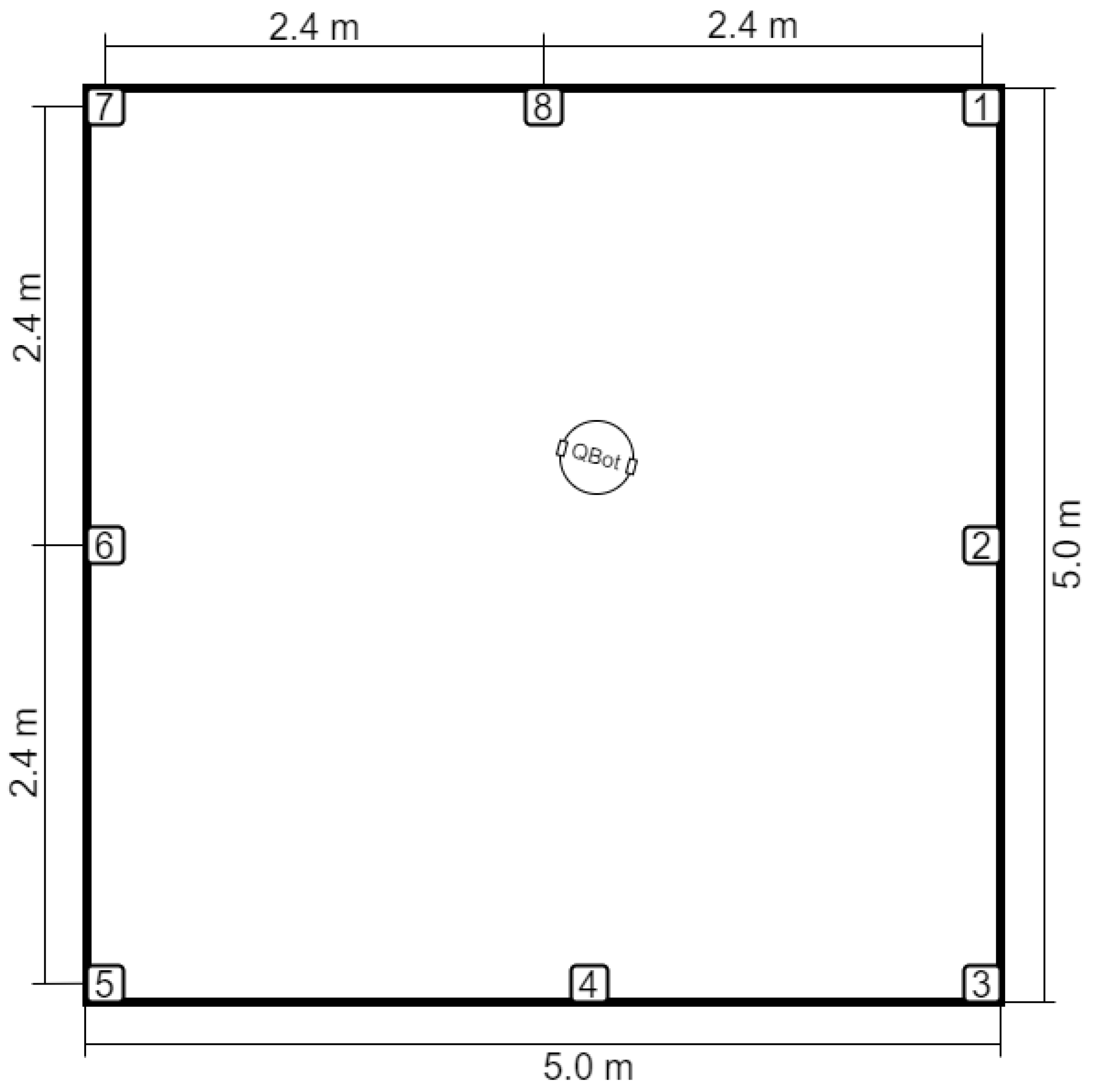
Figure 1. Dimensions of workspace with the arrangement of cameras.
Energies 16 01210 g001
Figure 2. Simulink diagram used to control the QBot 2e robot with the pure pursuit algorithm.
Energies 16 01210 g002
Figure 3. Energy used to complete the path for the specified parameter set number—track 1.
Energies 16 01210 g003
Figure 4. Time needed to path completion for the specified parameter set number—track 1.
Energies 16 01210 g004
Figure 5. Path matching accuracy for the specified parameter set number—track 1.
Energies 16 01210 g005
Figure 6. Cost function vs. linear speed for selected maximum values of the angular rate and look ahead distance—track 1.
Energies 16 01210 g006
Figure 7. Cost function vs. angular rate for selected maximum values of the linear speed and look ahead distance—track 1.
Energies 16 01210 g007
Figure 8. Cost function vs. look ahead distance for selected values of the linear speed and maximum angular rate—track 1.
Energies 16 01210 g008
Figure 9. Changes in angular rate over time for the lowest value of the cost function equal to 1—track 1).
Energies 16 01210 g009
Figure 10. Individual motor power and the total power over time, for the lowest value of the cost function equal to 1—track 1.
Energies 16 01210 g010
Figure 11. Desired path vs. actually traveled path for the lowest value of the cost function equal to 1—track 1.
Energies 16 01210 g011
Figure 12. Changes in angular rate over time for the mid value of the cost function equal to 1.0930—track 1.
Energies 16 01210 g012
Figure 13. Individual motor power and the total power over time, for the mid value of the cost function equal to 1.0930—track 1.
Energies 16 01210 g013
Figure 14. Desired path vs. actually traveled path for the mid value of the cost function equal to 1.0930—track 1.
Energies 16 01210 g014
Figure 15. Changes in angular rate over time for the highest value of the cost function equal to 1.2970—track 1.
Energies 16 01210 g015
Figure 16. Individual motor power and the total power over time, for the highest value of the cost function equal to 1.2970—track 1.
Energies 16 01210 g016
Figure 17. Desired path vs. actually traveled path for the highest value of the cost function equal to 1.2970—track 1.
Energies 16 01210 g017
Figure 18. Energy used to complete the path for the specified parameter set number—track 2.
Energies 16 01210 g018
Figure 19. Time needed to path completion for the specified parameter set number—track 2.
Energies 16 01210 g019
Figure 20. Path matching accuracy for the specified parameter set number—track 2.
Energies 16 01210 g020
Figure 21. Cost function vs. linear speed for selected maximum values of the angular rate and look ahead distance—track 2.
Energies 16 01210 g021
Figure 22. Cost function vs. angular rate for selected maximum values of the linear speed and look ahead distance—track 2.
Energies 16 01210 g022
Figure 23. Cost function vs. look ahead distance for selected values of the linear speed and maximum angular rate—track 2.
Energies 16 01210 g023
Figure 24. Changes in angular rate over time for the lowest value of the cost function equal to 0.8369—track 2.
Energies 16 01210 g024
Figure 25. Individual motor power and the total power over time, for the lowest value of the cost function equal to 0.8369—track 2.
Energies 16 01210 g025
Figure 26. Desired path vs. actually traveled path for the lowest value of the cost function equal to 0.8369—track 2.
Energies 16 01210 g026
Figure 27. Changes in angular rate over time for the mid value of the cost function equal to 1.0858—track 2.
Energies 16 01210 g027
Figure 28. Individual motor power and the total power over time, for the mid value of the cost function equal to 1.0858—track 2.
Energies 16 01210 g028
Figure 29. Desired path vs. actually traveled path for the mid value of the cost function equal to 1.0858—track 2.
Energies 16 01210 g029
Figure 30. Changes in angular rate over time for the highest value of the cost function equal to 1.3732—track 2.
Energies 16 01210 g030
Figure 31. Individual motor power and the total power over time, for the highest value of the cost function equal to 1.3732—track 2.
Energies 16 01210 g031
Figure 32. Desired path vs. actually traveled path for the highest value of the cost function equal to 1.3732—track 2.
Energies 16 01210 g032
Table 1. The variants of the parameters sets: linear velocity, angular rate and look ahead distance.
Parameter Set Number1234567891011121314
v (m/s)0.10.20.40.10.20.40.10.20.40.10.20.40.10.2
ω (rad · s 1 ) 0.30.30.30.60.60.60.90.90.90.30.30.30.60.6
L d (m)0.50.50.50.50.50.50.50.50.51.01.01.01.01.0
ParameterSetNumber15161718192021222324252627
v (m/s)0.40.10.20.40.10.20.40.10.20.40.10.20.4
ω (rad · s 1 ) 0.60.90.90.90.30.30.30.60.60.60.90.90.9
L d (m)1.01.01.01.01.51.51.51.51.51.51.51.51.5
Table 2. Variants of parameters (linear velocity, angular velocity, look ahead distance) for which the first path has not been completed.
Parameter Set Numberv (m/s) ω (rad · s 1 ) L d (m)
30.40.30.5
120.40.31.0
210.40.31.5
Disclaimer/Publisher’s Note: The statements, opinions and data contained in all publications are solely those of the individual author(s) and contributor(s) and not of MDPI and/or the editor(s). MDPI and/or the editor(s) disclaim responsibility for any injury to people or property resulting from any ideas, methods, instructions or products referred to in the content.