Thermal Diffusivity in the Subsoil: A Case Study in the Asturias (Northern Spain)

Abstract

This study presents a novel methodology for determining the apparent thermal diffusivity of subsoil in situ, employing two heat transfer models within the subsurface: one method is based on heat conduction caused by air temperature oscillations, while the other considers heat transmission via both conduction and convection due to groundwater flow. Differential equations were solved, and non-linear regression analysis was employed. This method has direct applications in various engineering and environmental domains, such as underground transmission lines, oil and gas pipelines, radioactive waste management, and geothermal systems, especially in the context of implementing horizontal geothermal collectors (HGC). The apparent thermal diffusivity value of 1.514 × 10⁻⁶ m² s⁻¹, within a 95% confidence interval spanning 1.512 × 10⁻⁶ m² s⁻¹ and 1.516 × 10⁻⁶ m² s⁻¹, was obtained from the section between 1.67 and 3.86 m depth in a research borehole located in Asturias, Northern Spain, using twenty-one temperature sensors. The method allowed for the calculation of the subsoil’s apparent thermal diffusivity up to a depth of 14.55 m.

1. Introduction

Thermal diffusivity quantifies a material’s ability to conduct heat relative to its heat storage capacity [1]. It serves as a core factor in the field of heat transfer, governing the rate at which heat propagates in response to temperature gradients [2], and is essential for various applications related to heat transfer, such as geothermal systems, construction, agriculture, biology, and more. Although its application is very broad, recent studies are mainly focused on geothermal systems.

While thermal conductivity is widely recognized as a fundamental parameter in the design of geothermal systems [3] and has been the subject of extensive research, the measurement and analysis of thermal diffusivity, another crucial property, require further investigation [4,5]. Ground thermal diffusivity exhibits considerable variability, influenced by factors such as soil type, density, and water content. Thermal diffusivity values can vary depending on the mineralogical composition of soils as well as on the differences in soil density and moisture. This implies that, for a given soil and depth, thermal diffusivity may fluctuate throughout the year, influenced by factors such as rainfall [6], with ground thermal diffusivity values ranging from 1.72 × 10⁻⁶ m²/s to 3.0 × 10⁻⁶ m²/s [7]. Authors [8] provided a range of values for sandy soil with a density of 1.46 × 10³ kg/m³, which varied between 0.3 × 10⁻⁶ m²/s and 1.1 × 10⁻⁶ m²/s based on its moisture content. Other authors have reported that thermal diffusivity measured in borehole cores, specifically in siltstones, varies from 1.1 × 10⁻⁶ m²/s to 1.6 × 10⁻⁶ m²/s [2].

Thermal diffusivity can be determined through measurements taken in soil samples using transient methods. The most commonly used method for soft rocks is the needle probe, initially described by [9,10]. In the case of hard rocks, measurements under transient conditions are conducted using flat or circular heat sources [11]. These methods can also be applied to borehole cores [2,12]. Various commercial devices and standardized [13] procedures are available for these measurements. The equipment used by [2], purchased from TCS Lippmann & Rauen Gbr, (Achim, Germany), allows for the measurement of both thermal conductivity and thermal diffusivity of samples or cores as small as 40 × 40 × 40 mm³ simultaneously. The thermal conductivity accuracy is 3%, with a measurement range of 0.2 to 25.0 W/mK, while the thermal diffusivity accuracy is 5%, with a measurement range of 0.6 to 0.6 to 3.0 × 10⁻⁶ s. However, such measurements have limitations as they only represent the specific core or sample, neglecting the subsurface’s inherent heterogeneity, such as the presence of multiple layers.

This problem can be addressed by using methods for measuring thermal diffusivity in situ. These methods can be grouped into two categories: The first system is based on the thermal response test (TRT), as presented in studies such as [3,4,14,15,16,17,18], among others. The second relies on extensive time series of naturally occurring ground temperature measurements at different depths, as discussed by [19,20,21,22,23,24,25,26,27,28]. In this system, a number of analytical, numerical, and experimental methods, developed based on the one-dimensional heat conduction equation, are available to determine soil thermal properties. Long-term temperature measurements in the subsurface are obtained by placing temperature sensors in a borehole and storing the data at specified intervals.

The analytical methods provide explicit equations for apparent thermal diffusivity based on the amplitude or phase of the temperature wave measured at different depths [29]. One of the first analytical methods for in situ estimation considered the first harmonic of daily waves, as widely discussed in [30]. A modified version of the amplitude method was proposed by [22]. Moreover, the so-called Arctangent method was proposed [31], which considers two harmonics. Authors used the amplitude method, in which the thermal diffusivity α in the depth interval z1–z2 is obtained by measuring the amplitudes of temperature waves A1 and A2 [2]. They applied the method in a borehole drilled in the Maritime Antarctic, using a chain of thermistors at various depths between 0.2 and 25 m. The temperature was measured every 5 min, and the data were stored in a datalogger. The same formula was used by [6] in temperature measurements taken in a geotechnical borehole drilled for the construction of a house in the south of Spain. Twenty-four sensors were placed 20 cm apart, and measurements were taken over the course of a year. Authors estimated diffusivity up to a depth of 10 m based on temperature data collected by three temperature sensors [32]. From a theoretical perspective, this method assumes that heat transfer occurs only through conduction in the vertical direction and that the ground is homogeneous and isotropic, with thermal diffusivity (α) not dependent on depth or time. Consequently, this can be calculated from ground temperatures by integrating the heat conduction equation, assuming that the temperature at the upper boundary is described by a sinusoidal function on a daily basis. However, natural grounds are heterogeneous, which is reflected in their physical properties.

The method called harmonic and numerical makes use of a large number of temperature measurements to implicitly solve for apparent thermal diffusivity. The numerical method is based on the evaluation of annual amplitude temperature decay and annual damping depth during long-term observation of the ground thermal disturbance diffusion resulting from the annual thermal flux at the ground surface [28]. The application of this method allowed [33] to estimate the apparent thermal diffusivity of the soil at depths of less than 2 m at two field sites in Melbourne based on temperature time series data collected at different depths.

Operating from a theoretical perspective, [34] conducted a study of subsurface temperature and its relationship with thermal diffusivity. The authors concluded that the depth at which the temperature in the borehole stabilizes and equals the annual mean ambient temperature depends on the thermal diffusivity of the subsurface.

In this work, a methodology is proposed for determining the thermal diffusivity in the subsurface, specifically in the shallower regions where significant temperature variations occur. This methodology applies regression methods to a time series of subsurface temperatures at different depths and the equation governing the heat transfer process in the subsurface. The subsurface’s thermal diffusivity is implicitly contained within this equation. Therefore, the regression yields the value of thermal diffusivity, which minimizes errors. In deriving the equation, two possibilities are considered: heat transfer in the subsurface due to conduction induced by temperature variations in the environment and heat transfer in the subsurface due to the combined effects of conduction and convection. In either case, the equations only represent the vertical component of heat flow.

The initial part of the article explains the derivation of the equations to be used and discusses the parameters within them. In the experimental section, the geothermal survey with the temperature measurement and recording system are described within the geological and hydrogeological context. Information from a gamma-ray log for the survey is available, and nearby water intake surveys provide insights into potential water levels in the borehole. The paper proceeds with sections dedicated to results, discussion, and ultimately presents the study’s conclusions.

2. Methodology and Results

The methodology has been structured into several sections. On one hand, in the Theoretical Background section, the search for the equation relating subsurface temperature to its thermal parameters is addressed. On the other hand, in the Site section, we emphasize the process of measuring subsurface temperature over an extended period in a specific geological and hydrogeological environment. These measurements were conducted in the context of a geothermal research pilot borehole located in Asturias, Northern Spain. Finally, in the Results section, we address the determination of which thermal parameters of the subsurface yield the best fit between actual temperature values and the derived equations. Calculations are performed for various soil layers, observed using core samples and geophysical records.

2.1. Theoretical Background Section

Temperatures in the subsurface can be influenced by various factors, such as the daily and seasonal fluctuations in air temperature as well as by the groundwater flow, while at deeper depths they are mainly determined by the geothermal gradient. In this work, we omit the latter factor and only consider temperatures in the upper layers of the subsurface, where temperature fluctuations are evident due to changes in ambient temperature and groundwater flow. In particular, Model I allows for the determination of the subsurface temperature at a specific depth and moment as a consequence of the vertical heat flow driven by conduction, resulting from the temperature difference between the subsurface and the external environment. Model II discusses the case of heat transmission in the subsoil due to the combined effect of heat transmission through conduction (solar radiation) and convection (underground water flow). In addition, it considers the heat flow due to the potential of the groundwater flow.

Model I also assumes:

• The ground surface is horizontal.
• The subsoil is composed of homogenous and isotropic layers.
• Subsoil temperature variations are a consequence of surface air temperature variations. Isotherms are horizontal.
• Heat flow is vertical.
• The air temperature T_a(t) as a function of time, t, can be described by a periodic function. This temperature is defined as a boundary condition to solve the main equation for conduction in the ground.

$$T_a\left(t\right)=T_m+A_0·\sin \left(\omega ·t-{\varnothing }_0\right)$$

(1)

where:

• T_m represents the average air temperature over period P,
• P denotes the period of the study,
• A₀ indicates the amplitude of air temperature during period P,
• ω stands for the angular frequency of the periodic variation, satisfying $\omega =\frac{2·\pi }{P}$,
• ${\varnothing }_0$ signifies the sinusoidal oscillation delay from the surface ground temperature at the beginning of the measurement period.

As is known, the vertical heat transport by conduction in a medium is mathematically represented as:

$$\frac{\partial T}{\partial t}=\alpha ·\frac{{\partial }^{2}T}{\partial z^2}$$

(2)

where $T$ represents the temperature of the porous medium, and $\alpha$ represents the bulk thermal diffusivity, defined as $\alpha =\raisebox{1ex}{$\lambda $}\!\left/ \!\raisebox{-1ex}{$\rho C_p$}\right.$, with $\lambda$ as the bulk thermal conductivity, and $\rho C_p$ as the volumetric heat capacity of the bulk porous medium.

The solution of the Equation (2), with the hypotheses indicated earlier and the boundary condition described in Equation (1), is the following:

$$T\left(z,t\right)-T_m=A_0·e^{-d·z}·sin\left(\omega ·t-{\varnothing }_0-d ·z\right)$$

(3)

where

$$d=\sqrt{\omega /\left(2·\alpha \right)}$$

The Equation (3) can be expressed as:

$$T\left(z,t\right)-T_m=A_{max,i}·sin\left(\omega ·t-{\varnothing }_i\right)$$

where:

$$A_{max,i}=A_0·e^{-d·z_i}$$

and

$${\varnothing }_i={\varnothing }_0+d ·z_i$$

The thermal diffusivity, $\alpha$, is incorporated into the expression for $d$, and it impacts both $A_{max,i}$ and ${\varnothing }_i$. This equation characterizes the model referred to as Model I.

In Model II, we account for the presence of water in the subsoil. In this scenario, the vertical component of the heat flow in the subsoil is additionally included and mathematically represented by Equation (4):

$$\frac{\partial T}{\partial t}=\alpha ·\frac{{\partial }^{2}T}{\partial z^2}-W·\frac{\partial T}{\partial z}$$

(4)

where $W$ is defined by the expression $W=\frac{C_w}{C_r}·u_z$, with $u_z$ representing the volumetric flow or the vertical component of Darcy velocity and assigned positive values as $z$ increases. Additionally, $C_w=4.186\times {10}^6 \mathrm{J}/{\mathrm{m}}^3$ represents the volumetric heat capacity of water, and $C_r$ is the volumetric heat capacity of rocks. While $C_w$ can be directly sourced from the literature, $C_r$ is intrinsic to the rock and needs to be determined for each specific case. Given that both $C_w$ and $C_r$ are specific to the rock, the term W is a function of $u_z$, and has units of velocity. The volumetric heat capacity of rock $C_r$ can be calculated from $n$, the porosity fraction of the rock, and $C_s$, the volumetric capacity of the solid components of the rock, as defined according to [35] with the following expression:

$$C_r=n·C_w+\left(1-n\right)·C_s$$

A general solution for Equation (4) is:

$$T\left(z,t, u_z\right)=B+A·e^{\left(a·z+b·t\right)}$$

(5)

where $a$ and $b$ are complex and constant numbers, while $B$ and $A$ are real numbers. By applying the boundary condition, it is demonstrated that $b=i·\omega$, $B=T_m$ and $A=A_o$. To determine the values of $a$ and $b$, the partial derivatives $\frac{\partial T}{\partial t}$,$\frac{\partial T}{\partial z}$ and $\frac{{\partial }^{2}T}{\partial z^2}$ are calculated from Equation (5). The obtained results are then substituted into Equation (4), resulting in:

$$b=\alpha ·a^2+W·a$$

(6)

Solving Equation (6) for $a$ yields two solutions:

$$a=\frac{-W\pm \sqrt{W^2+4·i·\alpha ·\omega }}{2·\alpha }=a_r+a_i·i$$

To obtain the values of $a_r$ and $a_i$, consider:

$$\sqrt{W^2+4·i·\alpha ·\omega }=r_r+r_i·i$$

where $r_r$ and $r_i$ are given by:

$$r_r=\frac{2·\alpha ·\omega }{\pm \sqrt{-W^2\pm \sqrt{\frac{W^4+16·{\alpha }^2·{\omega }^2}{2}}}}$$

$$r_i=\pm \sqrt{\frac{-W^2\pm \sqrt{W^4+16·{\alpha }^2·{\omega }^2}}{2}}$$

Consequently, the real and imaginary parts of $a$ are expressed as follows:

$$a_r=-\frac{W}{2·\alpha }+\frac{\sqrt{2}·\omega }{\sqrt{-W^2+\sqrt{W^4+16·{\alpha }^2·{\omega }^2}}}$$

$$a_i=-\frac{\sqrt{-W^2+\sqrt{W^4+16·{\alpha }^2·{\omega }^2}}}{2·\sqrt{2}·\alpha }$$

As a result, Equation (5) transforms into:

$$T\left(z,t, u_z\right)-T_m=A_0·e^{\left(\left(a_r+a_i·i\right)·z+i·\omega ·t\right)}=A_0·e^{\left(a_r·z\right)}·e^{\left(a_i·i·z+i·\omega ·t\right)}$$

By replacing the root signs and conducting a coherence study, the expression simplifies to:

$$T\left(z,t,u_z\right)-T_m=A_0·e^{-\left(-\frac{W}{2·\alpha }+\frac{\sqrt{2}·\omega }{\sqrt{-W^2+\sqrt{W^4+16·{\alpha }^2·{\omega }^2}}}\right)·z}·\sin \left(\omega ·t-{\varnothing }_0-\frac{\sqrt{-W^2+\sqrt{W^4+16·{\alpha }^2·{\omega }^2}}}{2·\sqrt{2}·\alpha }·z\right)$$

(7)

Here, we define:

$$M=\frac{1}{d}·\left[-\frac{W}{2·\alpha }+\frac{\sqrt{2}·\omega }{\sqrt{-W^2+\sqrt{W^4+16·{\alpha }^2·{\omega }^2}}}\right]$$

(8)

$$N=\frac{1}{d}·\left[\frac{\sqrt{-W^2+\sqrt{W^4+16·{\alpha }^2·{\omega }^2}}}{2·\sqrt{2}·\alpha }\right]$$

(9)

Equation (7) can be further expressed as:

$$T\left(z,t,u_z\right)-T_m=A_0·e^{-M·d·z}·\sin \left(\omega ·t-{\varnothing }_0-N·d·z\right)$$

(10)

This can be represented as:

$$T\left(z_i,t,u_z\right)-T_m=A_{max,i}^{\prime }·\sin \left(\omega ·t-{\varnothing }_i^{\prime }\right)$$

(11)

In this case, $A_{max,i}^{\prime }=A_0·e^{-M·d·z_i}$ and ${\varnothing }_i^{\prime }={\varnothing }_0+N·d·z_i$, where $M$ and $N$ are dimensionless variables dependent on $u_z$ and $\alpha$. In simpler terms, the thermal diffusivity $\alpha$ influences $d$, $M$ and $N$, while $u_z$ impacts $W$ and consequently to $M$ and $N$.

Equation (10) exhibits a resemblance to Equation (3). Both equations depict the temperature variation with depth. Therefore, temperature can be determined as the product of:

• An exponential function independent of time, dependent on depth and ground characteristics. This expression defines the maximum amplitude of the temperature in the subsoil.
• A periodic function that considers time in addition to the parameters mentioned above. This function characterizes the delay of the maximum temperature change in the subsurface.

Both functions differ in their arguments: $M$ only affects the temperature damping, and $N$ only affects the temperature delay. Both variables appear as factors multiplied by $d·z$. As indicated above, $M$ and $N$ depend on $u_z$ and $\alpha$. Hence, for a given lithology, if $u_z$= 0, $W=0$; then, $M$ and $N$ are equal to 1, and Equation (10) reduces to Equation (3).

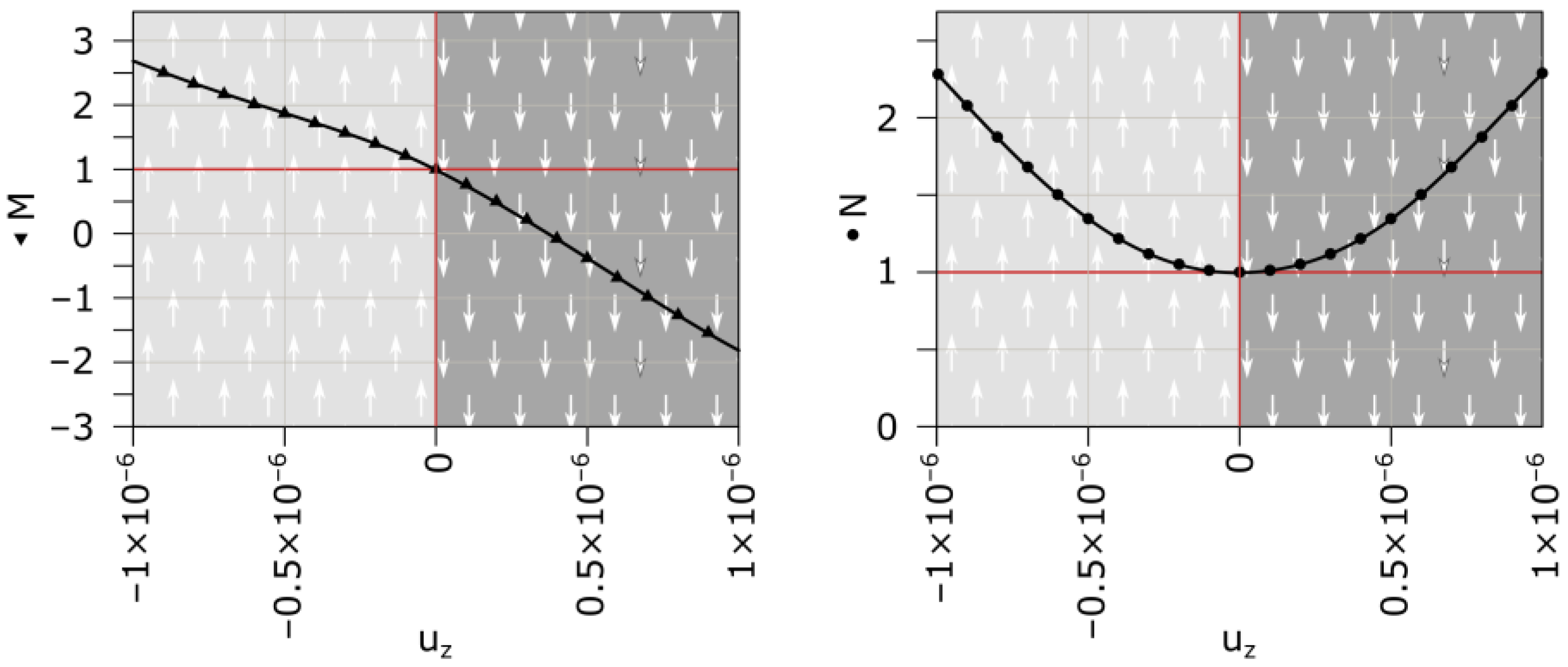
Then, a theoretical study of $M$ and $N$ is presented for the hypothetical case where the thermal diffusivity is set to 1 × 10⁻⁶ m²/s and the ratio $C_w/C_r$ is 1.85. Figure 1 represents the calculated values of M and N based on Equations (8) and (9) for a range of $u_z$ between −0.1 × 10⁻⁶ m/s and 0.1 × 10⁻⁶ m/s. These values are within a reasonable range, and this estimation provides insight into the behavior of M and N.

This figure illustrates that M consistently decreases with increasing $u_z$. Additionally, $M>1$ when $u_z<0$ and $M<1$ for $u_z>0$. In simpler terms, if the flow is upward, $M>1$, resulting in a lower value for $e^{-M·d·\left(z_j-z_i\right) }$ in Equation (10) compared to the case when M = 1. Conversely, when $M<1$, $e^{-M·d·\left(z_j-z_i\right)}$ is higher than it would be if $M=1$.

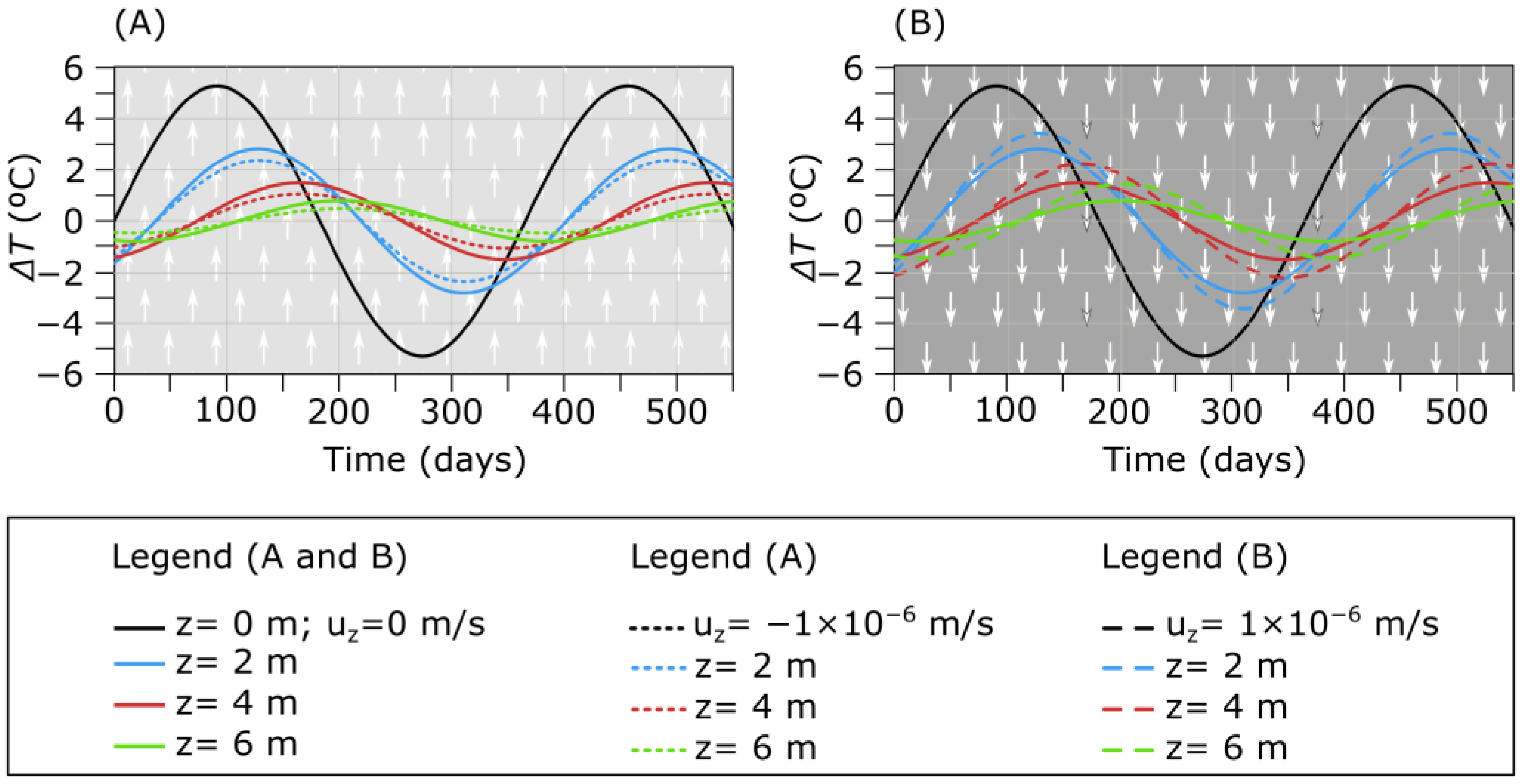
Figure 2 illustrates the theoretical temperature variation, represented as $T\left(z,t\right)-T_m\left(t\right)$, using Equation (3) (solid lines) and (10) (dashed lines) for different depths (0, 2, 4, and 6 m). In both cases, $A_0$ is set to 5.2 [°C], and ${\varnothing }_0$ is set to 0. When employing Equation (10), the values of $M$ and $N$ used in the equations are derived from Figure 1 by fixing the $u_z$ value. For Figure 2A, a $u_z$ value of −1 × 10⁻⁶ m/s is considered, and for Part B, the value is 1 × 10⁻⁶ m/s. For each depth z, the solid curves (Model I, Equation (3)) represent the maximum amplitude, $A_{max,i}$, as $\left[A_0·e^{\left(-d·z\right)}\right]$, with ${\varnothing }_i$ indicating $\left[d·z\right]$. In the case of the dashed curves (Model II, Equation (10)), the maximum amplitude is determined by $\left[A_0·e^{\left(-M·d·z\right)}\right]$, and ${\varnothing }_i$ corresponds to $\left[N·d·z\right]$.

In the case where $M>1$ ($u_z<0$, Figure 2A), the temperature amplitude variation would be less than what it would be if there were no water flow. In other words, the temperature is more damped than in the case of only heat transmission via conduction. Conversely, if $M<1$, ($u_z>0$, Figure 2B), the subsoil temperature is less damped. It appears that $M$ has a significant impact on temperature damping in the subsoil.

Figure 2 also shows that $N$ forms a parabola, with a minimum value of 1 corresponding to $u_z=0$. As $N$ is always greater than 1 and symmetric to the vertical axis, the effect of vertical groundwater flow depends only on the velocity value, not the flow direction.

Figure 2 indicates that the vertical velocity of water has a more pronounced effect on temperature amplitude than on the delay, which is negligible.

The delay is in the order of hours, which means it cannot be detected in curves where the horizontal axis represents days.

In both models, the general Equations (2) and (4) are solved using the boundary represented by Equation (1). However, the actual ambient temperature poorly aligns with Equation (1) due to various factors (clouds, rain, etc.). Fortunately, these external influences diminish with depth. To apply the previously presented methodology, Equation (1) is replaced by the boundary condition provided by Equation (12), representing the temperature at a specific depth $z_i$ in the same format as Equation (1).

$$T\left(z_i, t\right)=T_m{}_i+A_{0,i}·\sin \left(\omega ·t-{\varnothing }_0\right)$$

(12)

where

• T_mi is the average temperature at depth z_i,
• A_0,i is the amplitude at depth z_i, which was previously referred to as A_max,i.

With this boundary condition, the new Equation (13) replaces the previous Equation (3) in Model I.

$$T\left(z_j,t\right)-T_m{}_i=A_{0, i}·e^{-d·\left(z_j-z_i\right)}·sin\left(\omega ·t-{\varnothing }_0-d ·\left(z_j-z_i\right)\right)$$

(13)

For model II, Equation (10) takes the form:

$$T\left(z_j,t,u_z\right)-T_m{}_i=A_{0, i}·e^{-M·d·\left(z_j-z_i\right)}·\sin \left(\omega ·t-{\varnothing }_0-N·d·\left(z_j-z_i\right)\right)$$

(14)

The equations enable the determination of the thermal diffusivity of the subsoil, incorporated as the parameter $d$. If ${\alpha }_{A\left(i,j\right)}$ represents the diffusivity obtained from the analysis of $A_{0,i}$ between depths $\left(z_i, z_j\right)$, and ${\alpha }_{\phi \left(i,j\right)}$ represents the diffusivity derived from the analysis of ${\alpha }_{\phi \left(i,j\right)}$ between the same depths, these values can be calculated using the following equations:

$${\alpha }_{A\left(i,j\right)}=\frac{\omega ·{\left(z_i-z_j\right)}^2}{2·{\left[\ln \left(A_{0,i}/A_{0,j}\right)\right]}^2}$$

(15)

$${\alpha }_{\phi \left(i,j\right)}=\frac{\omega ·{\left(z_i-z_j\right)}^2}{2·{\left({\varnothing }_i-{\varnothing }_j\right)}^2}$$

(16)

The difference between the previous expressions lies in their respective denominators. Equation (15) relates to amplitudes, while Equation (16) concerns delays. Under Model I, the equations are expected to possess an equality, where $ln\left(\raisebox{1ex}{$A_{0,i}$}\!\left/ \!\raisebox{-1ex}{$A_{0, j}$}\right.\right)$ equals $\left[{\varnothing }_i-{\varnothing }_j\right]$. However, if the results do not match, this suggests Model I is unsuitable, making Model II applicable. Analyzing Figure 2 and the related calculations reveals that when $M>1$, ($u_z<0$, Figure 2A), the ratio surpasses 1, resulting in $\left[ln\left(\raisebox{1ex}{$A_{0,i}$}\!\left/ \!\raisebox{-1ex}{$A_{0, j}$}\right.\right)\right]$>$\left[{\varnothing }_i-{\varnothing }_j\right]$. Conversely, the ratio falls below 1 if $M<1$, ($u_z>0$).

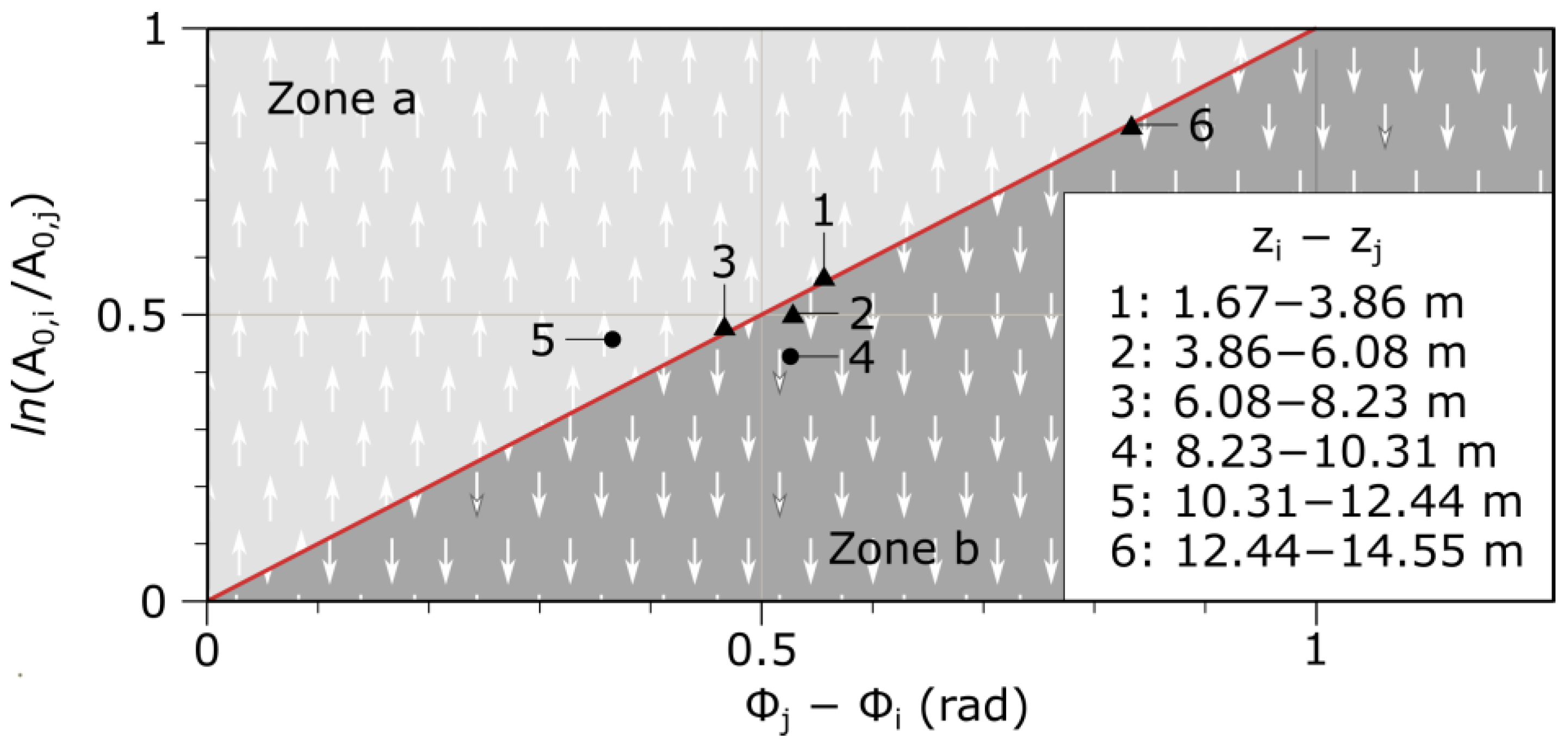
Figure 3 exhibits a graph illustrating the $ln\left(\raisebox{1ex}{$A_{0,i}$}\!\left/ \!\raisebox{-1ex}{$A_{0, j}$}\right.\right)$ values plotted against $\left[{\varnothing }_i-{\varnothing }_j\right]$ for various $u_z$ values, ranging from −1 × 10⁻⁶ m/s to 1 × 10⁻⁶ m/s. This graph is based on the dataset from a prior theoretical study. As previously mentioned, it includes a line with a slope of 45°, indicating instances where the value pairs relate to Model I. The lines positioned above the 45° line in the graph, referred to as Zone a, represent Model II with $u_z<0$. The background in this area is marked with upward-pointing arrows for clarity. Similarly, lines located below the 45° line, denoted as Zone b, signify the Model II with $u_z>0$. The graph’s background in this area is shaded with downward-pointing arrows.

The theoretical background has been covered before this point. The utility of these models lies in their straightforward application when subsurface temperature data at various depths are available. $A_{0,i}$ and ${\varnothing }_i$ are computed for diverse depths from this data, generating a graph like the preceding one. The calculated value pairs are charted and, based on their alignment with Zones a, b, or the 45-degree line, the respective equations of Models I and II are employed.

Subsequently, the underground temperature data are adjusted using non-linear regression methods to conform to the corresponding equations, yielding the sought-after parameters: thermal diffusivity for Model I and thermal diffusivity along with $u_z$ for Model II.

The method is suitable for depths where temperature fluctuations are detectable, typically within shallow depths that vary according to location-specific circumstances. A study published by [35] uses the term “convergence depth” for the depth at which the difference in temperature between the subsurface temperature at that depth and the annual average ambient temperature cannot be distinguished by a standard resolution temperature sensor. This convergence depth, typically around 20 m, determines the maximum applicable depth for the methodology presented in this paper. The ensuing sections demonstrate the practical application of these methods through a case study.

2.2. Site

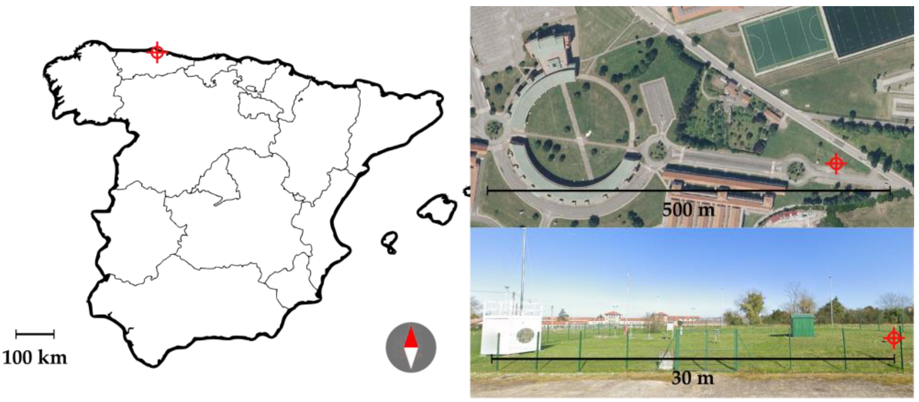
The previously displayed Models I and II were utilized to analyze an extensive series of temperature data measured and recorded within a geothermal pilot borehole at varying depths. The borehole, referred to as Q-Thermie, is positioned 26 m above sea level and 3 km from the coastline, situated within the Campus de Viesques, University of Oviedo (Gijón, Spain), at coordinates longitude 5°37′16″ W and latitude 43°31′23″ N, and is adjacent to a meteorological station operated by the State Meteorology Agency (Agencia Estatal de Meteorología, AEMET, Madrid, Spain) (Figure 4).

Some interesting characteristics of the borehole are detailed in

Table 1. Characteristics of the geothermal pilot borehole.

Drilling	Method	Diameter	Depth
	Rotation with continuous drilling core	125 mm	52 m
Geothermal pipes	Type	Diameter outside tube	Diameter inner tube
	Coaxial	50 mm	25 mm
Geothermal backfill	Type	Trademarck	Model
	Grout composition: silica sand and sulfate-resistant cement enhanced with additives	Energrout	Energrout HD 2.3

.

The Q-Thermie borehole is embedded within the Asturian Jurassic succession. This borehole intersects the “Gijon formation”, characterized by the alternation of marly limestone and grey dolomite [37].

The Gijon geological formation serves as a carbonate aquifer renowned for its high permeability, transmissivity, and storage coefficients, rendering its use expensive. However, the presence of loamy-clayey levels within the aquifer interrupts its hydraulic connection [37]. The drilling of cores allowed us to measure the porosity of the penetrated materials. A mercury injection porosimeter was used, determining the porosity to be 0.50%.

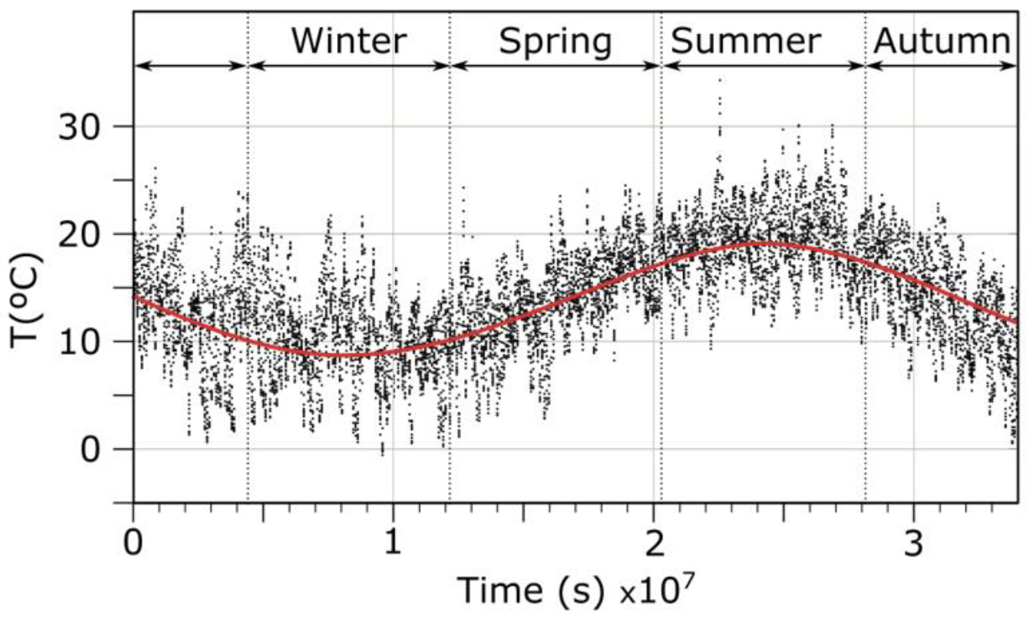
Figure 5 illustrates the recorded surface air temperature data obtained from the meteorological station (Meteorology State Agency, Government of Spain, AEMET) located adjacent to the pilot borehole over the observed period.

Prior to the installation of the geothermal probes, a gamma-ray probe from a Mount Sopris 3000 device was employed in the borehole. Figure 6 shows, among other aspects, the acquired gamma-ray log.

The central part of Figure 6 shows the positions of temperature sensors spaced about 2 m apart, ranging from 1.67 to 43.41 m in depth. The 2-m spacing between sensors was estimated before drilling and determined according to communication system requirements.

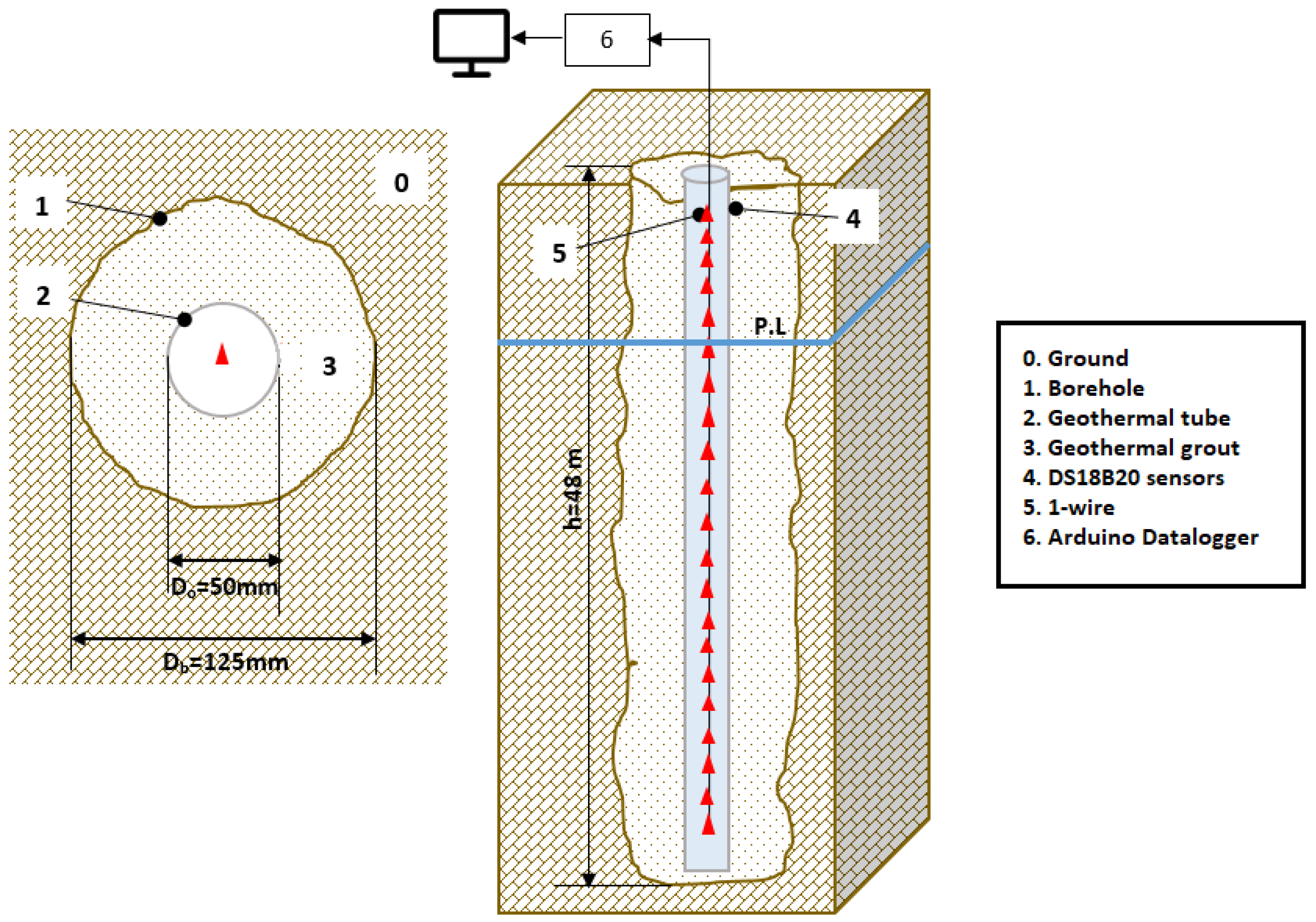
Temperature monitoring in the subsoil involves twenty-one DS18B20 temperature sensors connected via a 1-wire cable, placed in a borehole for long-term observation. A detailed description of the instrumentation is presented in [38], although we describe some of its features and limitations below.

The DS18B20 sensors (manufactured by Maxim Integrated, San José, CA, USA) supply 12-bit temperature readings. According to the manufacturer’s specifications, the standard sensitivity of sensors is 0.5 °C, and the mean standard error for the temperature range of 10 °C to 20 °C is between −0.45 and −0.11 °C. However, the manufacturer specifies that the sensitivity can be further enhanced through the individual calibration of each sensor. In this case, individual calibration has been performed on each sensor, resulting in a final sensitivity of ±0.06 °C within the subsurface temperature range.

The information is sent to/from the DS18B20 over a 1-wire interface, so that only one wire needs to be connected from a central microprocessor to the DS18B20 sensors. The sensors were connected to an Arduino-datalogger, programmed to record the temperature of each sensor. These sensors continuously recorded the temperature every five minutes over a period of one year. Figure 7 displays a sectional and depth view of the arrangement of the sensors (highlighted in red) within the borehole, attached to the 1-wire cable.

On the right side of Figure 6, temperature–depth profiles for specific months are displayed. The temperatures depicted are the average values recorded during the initial week of November, February, May, and August, respectively.

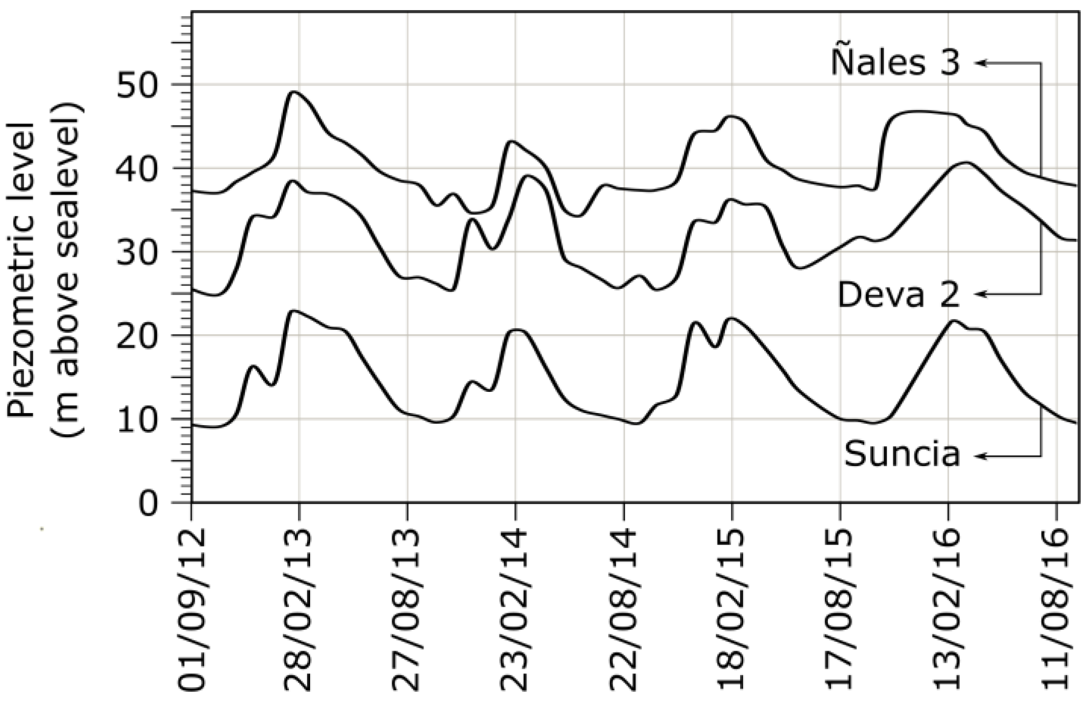
The Gijón municipal water company (Empresa Municipal de Aguas, EMA, Gijón, Spain) manages multiple boreholes providing water supply to Gijón, situated near the study area [39]. Figure 8 illustrates the positions of both EMA’s and Q-Thermie boreholes. The water level information about these boreholes is available for an extended period. These data are used to extract valuable information that is presented later in the Results section.

From the porosity of core samples y, $n$ was determined using a Hg injection porosimeter $\left(n=0.50\%\right)$. From study [40] $C_s=2.25\times {10}^6 \mathrm{J}·{\mathrm{m}}^{-3}{\mathrm{K}}^{-1}$, and $C_w=4.18\times {10}^6 \mathrm{J}·{\mathrm{m}}^{-3}{\mathrm{K}}^{-1}$, so volumetric heat capacity, $C_r=2.26\times {10}^6 \mathrm{J}·{\mathrm{m}}^{-3}{\mathrm{K}}^{-1}$.

2.3. Results

In this section, we present two key sets of results. First, we cover general findings from the borehole and its immediate surroundings. This includes air temperature analysis, the lithological column from the geothermal borehole, subsurface temperature trends with depth, and insights from the EMA’s boreholes. Then, we apply the methodology detailed in the Theoretical Background to determine the subsurface’s thermal properties in our case study.

The study of air temperature, as depicted in Figure 5, established an amplitude of $A_0=5.2 °\mathrm{C}$ and observed a temporal delay, ${\varnothing }_0$, between the theoretical sinusoidal function ($\Delta \mathrm{T}=0$ when $t=0 \mathrm{s})$ and the actual sinusoidal function. However, the $R^2$ value, as detailed in

Table 2. Fitting Surface Air Temperature data provided by [38] to Equation (1). SSE: sum of squared errors; $R^2$: R square; RMSE: root-mean-square error.

$${\mathit{A}}_0 \left[°\mathbf{C}\right]$$	$${\varnothing }_{\mathit{i}} \left[\mathbf{Days}\right]$$	SSE	$${\mathit{R}}^2$$	$${\mathit{R}}^2 \mathbf{A}\mathbf{j}\mathbf{u}\mathbf{s}\mathbf{t}\mathbf{e}\mathbf{d}$$	RMSE
5.224	4.84	0.4623	0.4623	0.4623	3.8560

, indicates a notably low fit, suggesting that employing this equation as a boundary condition may yield poor results. The graph (Figure 9) shows the best fitting curve, represented by the red curve in relation to Equation (1).

The stratigraphic sequence, deduced from continuous drilling core samples and the gamma-ray log, is visually presented in the Figure 6. The sequence of dolomite, limestone, marly limestone, and shale layers is clear. Dolomite predominates the uppermost zone notably. Extensive fracturing in the dolomite layers necessitated drilling from inside the casing.

From the analysis of underground temperatures depicted in Figure 6, it is inferred that temperatures converge around the 15 m depth mark, known as the convergence depth. Additionally, according to [35], the depth at which the heat flux reverses is observed to be approximately 5 m.

Figure 9 illustrates the values of $T\left(z_i,t\right)$ at various depths. A significant observation is the reduction in temperature amplitude with greater depth. Notably, at a depth of 20.14 m the temperature amplitude nearly reaches zero. Furthermore, the graph demonstrates a rightward delay as depth increases.

Table 3. Goodness of fit between the temperature data collected from various DS18B20 sensors and Equation (10).

${\mathit{z}}_{\mathit{i}} \left[\mathbf{m}\right]$	${\mathit{A}}_{0, \mathit{i}} \left[°\mathbf{C}\right]$	${\varnothing }_{\mathit{i}} \left[\mathbf{Days}\right]$	$\mathbf{S}\mathbf{S}\mathbf{E}$	${\mathit{R}}^2$	${\mathit{R}}^2 \mathbf{A}\mathbf{j}\mathbf{u}\mathbf{s}\mathbf{t}\mathbf{e}\mathbf{d}$	$\mathbf{R}\mathbf{M}\mathbf{S}\mathbf{E}$
$1.67$	3.86 (3.85, 3.85)	$24.16$	$9232$	$0.9965$	$0.9965$	$0.3152$
$3.86$	2.19 (2.19, 2.18)	$56.52$	$1211$	$0.9939$	$0.9939$	$0.1142$
$6.08$	1.32 (1.32, 1.32)	$87.54$	$483.2$	$0.9934$	$0.9934$	$0.07212$
$8.23$	0.81 (0.81, 0.81)	$114.61$	$293.6$	$0.9904$	$0.9904$	$0.05622$
$10.31$	0.53 (0.53, 0.53	$145.28$	$152.7$	$0.9893$	$0.9893$	$0.04055$
$12.44$	0.33 (0.33, 0.33)	$167.13$	$137.2$	$0.9764$	$0.9764$	$0.038$
$14.55$	0.14 (0.14, 0.14)	$219$	$292.2$	$0.7515$	$0.7515$	$0.056$

displays the $A_{0,i}$ and ${\varnothing }_i$ values obtained from temperature adjustments at various sensor depths, in alignment with Equation (10). It also includes coefficients (with 95% confidence bounds) and goodness of fit. Beyond 14.55 m in depth, the thermal gradient is so minor that changes are hardly noticeable. It is also observed that the correlation coefficient decreases with increasing depth.

Beyond 14.44 m in depth, the thermal fluctuations in the subsurface are so minimal that they are hardly noticeable, which worsens the fit and consequently the correlation coefficient.

During the month of September, for which the isopiestic lines are depicted as reported in Figure 8, the piezometric level is observed to be at its lowest level, as illustrated in Figure 10. By early March, it stabilizes between 7 and 13 m above this level.

The Q-Thermie borehole was drilled in early November, and the water level stabilized at a depth of 13 m, indicating that the piezometric level in the borehole was 13 m above sea level, consistent with the data from the EMA boreholes. The direction of water flow was inferred from this study.

Next, underground temperatures were analyzed to determine the thermal properties of the subsurface. The temperature data we analysed in accordance with three approaches to determine the apparent thermal diffusivity of the subsoil.

In the initial analysis, data from adjacent sensors were considered in order to calculate the pairs $ln\left(\raisebox{1ex}{$A_{0, i}$}\!\left/ \!\raisebox{-1ex}{$A_{0,j}$}\right.\right)$ and $\left[ {\varnothing }_i-{\varnothing }_j\right]$ using the $A_{0, i}$ and ${\varnothing }_i$ values from Table 3. The temperature data from greater depths were taken into account but are not shown because the temperature variations are so small that it is impossible to detect the amplitudes or delays.

The necessary pairs were generated to create a graph akin to that of Figure 3. These value pairs have been plotted in Figure 11.

Following the initial analysis, it is evident that points 1, 2, 3, and 6 align with the ‘conduction only’ line. As a result, Model I can be applied to temperatures within the ranges of 1.67–3.86 m, 3.86–6.08 m, 6.08–8.23 m, and 12.44–14.55 m, while Model II is suitable for temperatures within the depth range of 8.23–12.44 m.

In the second analysis, and $N_{i,j}$ values between depths $z_i$ and $z_j$ were estimated using a minimization approach based on Equation (10).

This involved directly measuring $T\left(z_j,t,u\right)$ and using the determined values of $A_{0, i}$ and $T_m{}_i$ (as indicated in Table 3). The resulting values for $M_{i,j}$ and $N_{i,j}$ and $R^2$ are presented in

Table 4. Values of $M_{i,j}$ and $N_{i,j}$ derived from Equation (12) for depths between $z_i$ and $z_j$.

$$\mathbf{Depth} \mathbf{of} \mathbf{Sensors} {\mathit{z}}_{\mathit{i}}, {\mathit{z}}_{\mathit{j}}$$	$${\mathit{M}}_{\mathit{i},\mathit{j}}$$	$${\mathit{N}}_{\mathit{i},\mathit{j}}$$	$${\mathit{R}}^2$$
1.67–3.86	1.056	1.037	0.9939
3.86–6.08	1.119	1.179	0.9934
6.08–8.23	1.148	1.103	0.9904
8.23–10.31	0.9317	1.152	0.9893
10.31–12.44	1.306	1.072	0.9764
12.44–14.55	1.281	1.285	0.9157
14.55–16.72	0.6234	1.031	0.4793
16.72–18.01	0.2542	0.5492	0.1553

.

From the analysis of the correlation coefficients presented in this table, it can be inferred that the reliability of the M and N values diminishes with increasing depth. Specifically, $R^2$ is greater than 0.9 down to a depth of 14.55 m, and even greater than 0.99 up to almost 10.31 m. However, it decreases to 0.47 at a depth of 14.55 m. For this reason, results at depths greater than 14.55 m are not considered and are excluded from the study.

Based on the information provided in this table, the subsoil within the depth range of 10.31–12.44 m exhibits a significantly higher value of $M_{i,j}$ than 1, which corresponds to the upward flow zone (Figure 11). Conversely, the section spanning 8.23–10.31 m displays an $M_{i,j}$ value noticeably below 1, consistent with a zone of descending flow, as indicated in Figure 1. The remaining sections have $M_{i,j}$ values that are nearly equal to 1.

Moreover, the N values consistently exceed 1, although the differences were not statistically significant.

In a third analysis, thermal diffusivity was estimated using Model I and Model II.

Based on the previous outcomes, Model I was applied to subsurface temperature data within the depths of 1.67–3.86 m; 3.86–6.08 m; 6.08–8.23 m; and 12.44–14.55 m, while Model II was used for temperatures recorded between depths of 8.23–12.44 m. Figure 12 illustrates the evolution of $\Delta T=T\left(z_j,t\right)-T_{m,i}$ against $t$ for the four mentioned intervals, derived from Equation (11), with the best-fitting curve obtained through the optimization procedure shown in red.

Regression analysis enables the determination of thermal diffusivity with a 95% confidence interval. The fit results and the coefficients indicating the goodness of the fit are presented in

Table 5. Thermal diffusivity ${\alpha }_{i,j}$ obtained for the intervals between the indicated depths using Equation (13) (Model I).

$$\mathbf{Sensor} \mathbf{Depths} {\mathit{z}}_{\mathit{i}}, {\mathit{z}}_{\mathit{j}}$$ (m)	$${\mathit{\alpha }}_{\mathit{i},\mathit{j}}\left[{\mathbf{m}}^2{\mathbf{s}}^{-1 }\right]$$	$$\mathbf{S}\mathbf{S}\mathbf{E}$$	$${\mathit{R}}^2$$	$${\mathit{R}}^2 \mathbf{A}\mathbf{j}\mathbf{u}\mathbf{s}\mathbf{t}\mathbf{e}\mathbf{d}$$	RMSE
1.67−3.86	1.51 × 10−6 (1.51 × 10−6, 1.52 × 10−6)	1211	0.9938	0.9938	0.1147
3.86−6.08	1.81 × 10−6 (1.80 × 10−6, 1.81 × 10−6)	513.7	0.993	0.993	0.07436
6.08−8.23	2.03 × 10−6 (2.03 × 10−6, 2.04 × 10−6)	299.6	0.9902	0.9902	0.05679
12.44–14.55	0.64 × 10−6 (0.64 × 10−6, 0.64 × 10−6)	76.49	0.9223	0.9223	0.029

for the specified intervals. The correlation coefficient in the uppermost layers exceeds 0.99 with a considerably narrow confidence interval.

Using [14], we applied Model II within the depth range from 8.23 m to 12.44 m allowed for the estimation of thermal diffusivity ${\alpha }_{i,j}$, and $u_z$. Figure 13 illustrates the measured $\Delta T=T\left(z_j,t,u_z\right)-T_m{}_i$ values for the sensors, along with the best-fitting red curve.

Similar to the previous case, regression analysis was used to determine the thermal diffusivity within a 95% confidence interval.

Table 6. Thermal diffusivity ${\alpha }_{i,j}$ obtained for the intervals between the indicated depths using Equation (12) (Model II).

$$\mathbf{Sensor} \mathbf{Depths} {\mathit{z}}_{\mathit{i}}, {\mathit{z}}_{\mathit{j}}$$ (m)	$${\mathit{\alpha }}_{\mathit{i},\mathit{j}}\left[{\mathbf{m}}^2{\mathbf{s}}^{-1 }\right]$$	$$\mathbf{S}\mathbf{S}\mathbf{E}$$	$${\mathit{R}}^2$$	$${\mathit{R}}^2 \mathbf{A}\mathbf{j}\mathbf{u}\mathbf{s}\mathbf{t}\mathbf{e}\mathbf{d}$$	RMSE
8.23−10.31	1.51 × 10−06 (1.51 × 10−06, 1.52 × 10−6)	152.7	0.9893	0.9938	0.1147
10.31−12.44	3.13 × 10−06 (3.11 × 10−06, 3.14 × 10−06)	137.2	0.9764	0.993	0.07436

displays the fitting results and the corresponding goodness-of-fit coefficients for the specified intervals. In this case, the correlation coefficients are comparatively lower. The correlation coefficient decreases with depth due to the reduced variance between the minimum and maximum temperatures.

The application of Model II to the subsurface temperature records at the specified depths enables the determination of $u_z{}_{i,j}$ alongside the thermal diffusivity. In this case of consecutive layers, calculations for $u_z{}_{i,j}$ were conducted for the entire range from 8.23 m to 12.44 m, treating this range as a single hydrogeological unit. The fitting results for $u_z{}_{i,j}$ are presented in

Table 7. $u_z$ values for deep intervals using Equation (14).

Sensor Depths (m)	${\mathit{u}}_{\mathit{z}}{}_{\mathit{i},\mathit{j}} \left[\mathbf{m} {\mathbf{s}}^{-1}\right]$	SSE	R2	Adjusted R2	RMSE
$8.23-12.44$	0.20 × 10−07 (0.19 × 10−07, 0.20 × 10−07)	137.9	0.9763	0.9763	0.03853

.

3. Discussions

The proposed models (Model I and Model II) provided significant results in the analysis of thermal diffusivity in the subsurface. They showed the prevalence of heat transmission through conduction in shallow layers and the more significant influence of convection in deeper layers. The values obtained for thermal diffusivity reflect excellent accuracy at all depths. For instance, in the range between 1.67 and 3.86 m, applying Model I yielded a thermal diffusivity of 1.514 × 10⁻⁶ m² s⁻¹ with a 95% confidence interval between 1.512 × 10⁻⁶ m² s⁻¹ and 1.516 × 10⁻⁶ m² s⁻¹, representing an accuracy of 0.264%. This highlights the robustness and high precision of the proposed method, surpassing commercial equipment precision.

It is important to emphasize that the methodology used is valid only up to a certain depth, known as the convergence depth, where thermal oscillations become indiscernible. The depth varies based on the subsurface’s thermal diffusivity, which, in this study, was observed at 14 m. The various types of TRT procedures can be employed for in situ determination of thermal diffusivity in deeper zones.

It is noteworthy that, in this work, the temperature sensors were distributed in sections determined by their position, without a precise representation of the different lithologies encountered. In future research, positioning the temperature sensors more appropriately in terms of lithological sections will provide a more detailed characterization.

The calculation of the vertical component of Darcy velocity yielded notable values, indicating very low vertical hydrodynamic flow ($u_z{}_{i,j}=$0.20 × 10⁻⁷ m s⁻¹) typical of low-permeability terrains, as encountered in the study case. The determination of the piezometric level was performed indirectly by consulting neighboring borehole piezometric levels, showing consistency between both results. There is a recognized need for more precise control of the piezometric level around the borehole to enhance the understanding of subsurface hydrology and, therefore, geothermal model precision.

4. Conclusions

The study underscores the importance of considering thermal models that incorporate both conduction and convection in the analysis of heat transport in the subsurface. The validated models allow for the determination of thermal diffusivity in various shallow subsurface sections. The high precision of the proposed method for measuring thermal diffusivity, as evidenced by the narrow confidence intervals and the representativeness of a range of sample values, highlights its superiority over standard laboratory equipment and its ability to more faithfully represent the characterized terrains.

A comparison with literature values demonstrates the method’s capability to provide more precise and detailed measurements than conventional approaches, making it a valuable tool for understanding subsurface thermal behavior in various contexts and depths. Additionally, it suggests a need for more comprehensive research in order to better understand the behavior of Darcy velocity and its relation to thermal diffusivity in different geothermal contexts. This deeper exploration could provide additional insights into hydrodynamic flow dynamics and their influence on subsurface heat transport, thereby enhancing the overall understanding of geothermal processes and their practical applications.