Forecasting of Solar Power Using GRU–Temporal Fusion Transformer Model and DILATE Loss Function

Abstract

Solar power is a clean and sustainable energy source that does not emit greenhouse gases or other atmospheric pollutants. The inherent variability in solar energy due to random fluctuations introduces novel attributes to the power generation and load dynamics of the grid. Consequently, there has been growing attention to developing an accurate forecast model using various machine and deep learning techniques. Temporal attention mechanisms enable the model to concentrate on the critical components of the input sequence at each time step, thereby enhancing the accuracy of the prediction. The suggested GRU–temporal fusion transformer (GRU-TFT) model was trained and validated employing the “Daily Power Production of Solar Panels” Kaggle dataset. Furthermore, an innovative loss function termed DILATE is introduced to train the proposed model specifically for multistep and nonstationary time series forecasting. The outcomes have been subjected to a comparative analysis with alternative algorithms, such as neural basis expansion analysis for interpretable time series (N-BEATS), neural hierarchical interpolation for time series (N-HiTS), and extreme gradient boosting (XGBoost), using several evaluation metrics, including the absolute percentage error (MAE), mean square error (MSE), and root mean square error (RMSE). The model presented in this study exhibited significant performance improvements compared with traditional statistical and machine learning techniques. This is evident from the achieved values of MAE, MSE, and RMSE, which were 1.19, 2.08, and 1.44, respectively. In contrast, the machine learning approach utilizing the Holt–Winters method for time series forecasting in additive mode yielded MAE, MSE, and RMSE scores of 4.126, 29.105, and 5.3949, respectively.

1. Introduction

In recent times, there has been an increased utilization of renewable energy sources, such as photovoltaic (PV) technology and analogous innovations, on a global scale [1]. The extensive adoption of solar power systems is presently hindered by a multitude of factors encompassing meteorological conditions, seasonal fluctuations, intrahourly irregularities, topographical elevation, and intermittent energy generation patterns. To address the operational expenditures arising from the necessity of energy reserves or potential deficiencies in electricity provisioning from PV systems, operators are compelled to proactively gather solar energy production data. As a consequence, solar power forecasting emerges as a pivotal and foundational component essential for the establishment of a dependable and steadfast solar energy sector. In particular, real-time predictions within intrahour intervals are of paramount significance for monitoring and dispatching functions, while anticipatory forecasts spanning intraday and day-ahead periods assume a crucial role in orchestrating spinning reserve capacity and the effective management of grid operations. Rooftop solar systems stand out as a highly promising source of energy for prosumers residing in densely populated metropolitan areas, owing to their growing popularity as demonstrated by the increasing installation of photovoltaic panels [2]. Empirical investigations have demonstrated that rooftop photovoltaic systems have the potential to meet the majority, if not all, of the electricity requirements of prosumers, suggesting that self-sustaining cities are likely to play a leading role in the era of energy transition [3]. Time series data often exhibit seasonal patterns or trends that can be difficult to capture using traditional recurrent neural networks. While long short-term memory (LSTM) networks have successfully captured long-term dependencies in time series data, they can still struggle with determining the relevant information to remember [4]. The temporal fusion transformer (TFT) has emerged as a deep neural network architecture for multihorizon time series forecasting in recent studies. This attention-based model effectively incorporates LSTM units within its framework to enhance its predictive capabilities. It combines the power of attention mechanisms with the ability to identify long-term relationships in time series data, making it well suited for various forecasting applications. It can directly learn patterns during training and provide advantages concerning interpretability. Additionally, TFT minimizes a quantile loss function, enabling it to produce a probabilistic forecast with a confidence interval. TFT has garnered recent attention in the domain of forecasting critical variables, manifesting in applications such as wind speed prediction [5], multistep forecasting of freeway traffic speed [6], day-ahead PV power forecasting [7], short-term electricity load forecasting [8], prognosticating high-speed train wheel wear [9], stock price prediction [10], nitrate levels forecasting in an aquaponics environment [11], and forecasting of economic systems [12]. The researchers in [5] employed TFT as an innovative attention-based deep learning framework that combines proficient multihorizon prediction capabilities with explicable insights for forecasting wind speed. The proposed VMD-ADE-TFT model was subjected to rigorous evaluation using a diverse set of eight real-world 1-h wind speed datasets. The demonstrated stability and precision of the VMD-ADE-TFT model in wind speed forecasting underscore its meritorious performance. In another study [6], authors employed the TFT model to forecast traffic speed. This architecture possesses the ability to capture both brief and protracted temporal dependencies through a multihead attention mechanism. Notably, TFT exhibited superior predictive performance in forecasting traffic speed 1 h in advance when compared with alternative models. In a comparable study [7], TFT was subjected to rigorous examination for its efficacy in predicting hourly day-ahead PV energy production. The empirical assessments were conducted on datasets from diverse facilities in Germany and Australia. The findings of this inquiry encompass a comprehensive comparative analysis, pitting TFT against other prominent algorithms, including ARIMA, long short-term memory (LSTM), multilayer perceptron (MLP), and XGBoost. These long short-term memory (contrasting) algorithms have been evaluated using established statistical error indicators.

To ensure the safety and dependability of railway systems, a pioneering framework rooted in transformer architecture, featuring multiplex local–global temporal fusion (LGF-Trans), has been employed to prognosticate the wheel wear condition of high-speed trains through the analysis of vibration signals [9]. Empirical investigations conducted on authentic operational data pertaining to CRH1A high-speed trains (HSTs) evince the capacity of LGF-Trans to accurately forecast wheel wear progression, surpassing the efficacy of contemporary deep learning methodologies.

A recent study [10] employed the TFT model alongside support vector regression (SVR) and LSTM models to forecast stock prices. The performance evaluation of each model centers upon two discerning metrics: mean square error (MSE) and symmetric mean absolute percentage error (SMAPE). The empirical findings underscore the superiority of the TFT model, as evidenced by its attainment of the most minimal predictive errors. The authors of [11] applied the TFT model to forecast nitrate levels in an aquaponics environment. A dataset pertinent to aquaponics, featuring time-varying attributes and a substantial volume of input entries, was employed to validate and extensively scrutinize the proposed approach. The empirical findings clearly illustrate noteworthy enhancements of the suggested model compared with foundational models, as evidenced by improvements in mean absolute error (MAE), MSE, and explained variance metrics, specifically in the context of 1-h sequential forecasts. The authors of [12] integrated the state-of-the-art TFT model within the realm of economic system prognostication, capitalizing on the significant congruence between deep learning methodologies and the intricate nonlinear attributes inherent in socioeconomic systems. They conducted an empirical prognostication of monthly output indicators within the context of the Chinese macroeconomic milieu. Performance analysis reveals pronounced merits of TFT outcomes over conventional benchmark models, including but not limited to ARIMA, BP, LSTM, TCN, and N-BEATS. The TFT framework has found application within the medical domain, notably in the realm of long-term prediction of emergency department overcrowding, as evidenced by Caldas et al. [13].

This study aims to predict PV power generation using a GRU–temporal fusion transformer (GRU-TFT) as the forecasting method. TFT incorporates interpretable explanations of temporal dynamics and high-performance forecasting over multiple horizons, using specialized components to select important attributes and gating layers to remove nonessential elements. This method potentially enhances the accuracy of forecasts compared with other methods by learning short- and long-term temporal relationships, which can benefit the management of PV production systems and the stability and operation of the power system.

The proposed GRU-TFT model was trained and validated employing the “Daily Power Production of Solar Panels” Kaggle dataset. The results have been compared with other algorithms, like neural basis expansion analysis for interpretable time series (N-BEATS), neural hierarchical interpolation for time series (NHiTS), and XGBoost, using several evaluation metrics, including MAE, MSE, and root mean square error (RMSE). This paper presents several contributions in the field of time series forecasting using deep learning methods:

• First, the authors introduce a novel variant of the TFT model, called GRU-TFT, in which gated recurrent unit (GRU) layers have replaced the LSTM layers in the LSTM encoder and decoder. The GRU-TFT model is evaluated, and its performance is compared with the original TFT model. GRU’s advantage is its combined forget and input gates into a single update gate. This allows it to capture short-term dependencies more effectively and model sequences with rapid changes.
• Second, the authors investigate the relationship between the number of attention heads and the RMSE of the model. They conduct experiments with different numbers of attention heads and analyze the impact on the model’s performance.
• Additionally, the distortion loss including the shape and time (DILATE) loss function is proposed as a strategic enhancement to address the issue of prediction latency arising from the utilization of the MSE loss function.
• Finally, the performance of the GRU-TFT model has been comprehensively evaluated using various metrics, like MAE, MSE, and RMSE.
• The results of the Diebold–Mariano test indicate that the proposed GRU-DILATE-TFT model exhibits statistically significant improvements in accuracy when compared with the XGBoost, NHiTS, and N-BEATS models, as evidenced by p-values below the predetermined significance level of 0.05.

This paper provides valuable insights into the design and assessment of deep learning architectures for predicting time series data with a particular focus on the TFT and GRU-TFT models. The contributions of this paper have the potential to inform future research in this area and advance state-of-the-art time series forecasting comparing its performance with other commonly used methods in the literature.

The paper is structured as follows: Section 2 provides a summary of the related work and state-of-the-art methods for PV forecasting, including those that utilize machine learning and deep learning-based models. Section 3 outlines the dataset preprocessing pipeline, the proposed model, and the underlying methodologies employed to develop it. Section 4 presents the dataset, results, and discussion. Lastly, Section 5 presents the study’s key conclusions and offers suggestions for future research directions.

2. Related Work

Numerous methodologies have been suggested to address the challenge of forecasting energy production within PV systems. This section is devoted to a comprehensive exploration of prior research endeavors and the present scholarly landscape concerning the development and advancements of PV power forecasting systems leveraging the capabilities of artificial intelligence (AI) approaches. In a recent study [7], TFT has undergone a systematic and thorough investigation into its effectiveness in the prediction of hourly day-ahead PV energy generation. The outcomes of this investigation encompass an exhaustive comparative evaluation, wherein TFT is compared against other prominent computational algorithms, notably including ARIMA, LSTM, multilayer perceptron (MLP), and XGBoost. These divergent algorithms underwent thorough examination utilizing well-established statistical metrics to assess their predictive performance.

Serrano et al. [14] developed two multivariate fuzzy time series (FTS) for short-term solar PV generation forecasting. The outcomes of this study reveal that the indirect prediction approach yields superior results when correlated with GHI, as opposed to the power simulation technique.

Almonacid et al. [15] devised an innovative approach grounded in dynamic artificial neural networks for the prediction of global solar irradiance and air temperature for a forthcoming 1-h interval. The findings from their investigation highlight the potential utility of the proposed methodology in accurately forecasting the power output of PV systems with a satisfactory level of precision for a 1-h lead time. A novel approach was introduced by Wang et al. [16] for day-ahead PV power forecasting. The approach integrates deep learning techniques with temporal correlation principles within the context of a partial daily pattern prediction (PDPP) framework. A comprehensive PDPP framework is formulated, which furnishes precise predictive insights into the daily patterns for specific days. The simulation outcomes underscore the superior accuracy of the proposed forecasting technique when augmented with time correlation adjustments (TCMs) as compared with the standalone LSTM-RNN model. Li et al. [17] introduced an innovative hybridized deep learning architecture, integrating wavelet packet decomposition (WPD) and LSTM networks, to enable the accurate prediction of PV power output with a 1-h forecast horizon. Empirical findings using a real-world PV system situated in Australia underscore the superior performance of the WPD-LSTM hybrid model when compared with other prominent deep learning methodologies, including LSTM, gated recurrent unit (GRU), recurrent neural network (RNN), and MLP. In another study, Pan et al. [18] introduced an innovative ultra-short-term predictive model for PV power generation. The model’s efficacy is enhanced through the incorporation of the max–min ant colony optimization (ACO) algorithm, the differential evolution algorithm, and an adaptive factor, thus creating an improved hybrid framework. The findings demonstrate that by employing thoughtful data preprocessing techniques, substantial enhancements are observed in the accuracy of forecasting nighttime and peak power output. Mellit, A., A. Massi Pavan, and V. Lughi. [19] developed and compared various types of deep learning neural networks (DLNN) for the purpose of short-term output forecasting of PV power. These DLNN models encompass LSTM, bidirectional LSTM (BiLSTM), GRU, bidirectional GRU (BiGRU), and the one-dimensional convolutional neural network (CNN1D). Additionally, hybrid architectures such as CNN1D-LSTM and CNN1D-GRU have been explored. The outcomes of this investigation reveal that the examined DLNNs exhibit noteworthy levels of accuracy, particularly in scenarios characterized by a 1-mi time horizon for one-step ahead forecasting. Addressing the challenges posed by the notable stochastic variability and relatively modest predictive precision observed in photovoltaic power generation, in a recent study, Li, Guohui, Xuan Wei, and Hong Yang. [20] introduced a novel forecasting framework denoted as WVMD-GTO-LSTM-EC. The framework integrates a multifaceted predictive model, leveraging the synergistic application of fuzzy C-means (FCM) clustering, enhanced variational mode decomposition (VMD) optimized through a white shark optimizer (WSO), LSTM networks fine-tuned by the artificial gorilla troops optimizer (GTO), and an error correction (EC) mechanism. The empirical findings robustly illustrate that the predictions generated by the WVMD-GTO-LSTM-EC model closely align with the actual observations, as evidenced by a notably high coefficient of determination (R = 0.99) and minimal values of mean absolute percentage error (MAPE), MAE, and RMSE. Khan et al. [21] introduced a novel dual-stream network designed to enhance the precision of PV forecasting. It is worth noting that the dual-stream network, coupled with its sophisticated feature selection mechanism, constitutes an innovative and pioneering approach within the realm of time series analysis, specifically tailored to the domain of PV power forecasting. The outcomes of these experiments distinctly showcase the superior predictive accuracy of our proposed model in comparison with prevalent state-of-the-art models. In a recent study [22], the authors introduced a novel two-stage ensemble model for predicting daily carbon emissions in the power industry. To address the challenge of modeling complexity, the authors employed the STL algorithm to reduce complexity in the modeling process. Furthermore, they leveraged metaheuristic algorithms to obtain optimal values for the model’s hyperparameters.

The authors demonstrated that the integration of knowledge distillation and the decomposition-ensemble approach significantly enhanced the forecasting performance. Cai et al. [23] devised an innovative decomposition-ensemble framework by integrating the variational mode decomposition method, econometric forecasting techniques, and deep learning methodologies. This framework was specifically designed to capture the inherent data characteristics of hourly PM2.5 concentrations. The developed forecasting framework exhibits promising potential for monitoring and predicting air quality conditions, particularly concerning PM2.5 concentration. By offering a theoretical foundation and technical support, this framework can aid in the formulation of effective strategies by governmental entities aimed at mitigating PM2.5 levels. The authors of [24] presented a novel cybersecure forecasting model, referred to as federated deep learning, which is specifically designed for predicting PV power generation in diverse regions throughout Iran. The obtained results highlight the exceptional precision and generalizability of the global cybersecure supermodel in accurately forecasting PV power generation across different regions. The precise prediction of wind power is of utmost importance in the effective management of wind power systems. In this regard, Hanifi et al. [25] devised a hybrid forecasting approach utilizing the WPD, LSTM, and CNN to enhance the accuracy of wind power forecasting. The outcomes of their study reveal the superior performance of their proposed model in comparison with seven alternative forecasting models.

Other forecasting models’ shortcomings are adequately addressed by the provided model. The limitations of the models it has replaced include difficulties in capturing long-term dependencies in time series data and difficulties in handling seasonal patterns as some models face challenges in handling complex seasonal patterns, resulting in suboptimal performance, inability to model dynamic relationships, sensitivity to outliers as TFT employs robust mechanisms to reduce the impact of outliers, and scalability issues as some forecasting models may encounter scalability issues. TFT’s parallel-processing transformer architecture provides greater scalability, making it suitable for handling complex datasets.

It has also introduced notable modifications. For instance, it replaces the conventional LSTM layers in both the encoder and decoder of the TFT model with GRU layers. One notable advantage of GRU is its consolidation of the forget and input gates into a single update gate, enabling it to more efficiently capture short-term dependencies and effectively model sequences characterized by rapid changes. Furthermore, to overcome the prediction latency associated with employing the mean square error (MSE) loss function, the authors proposed a novel enhancement known as the distortion loss including the shape and time (DILATE) loss function. This strategic addition aims to address the aforementioned issue.

3. Materials and Methods

This section provides a concise overview of the dataset utilized for training and evaluating the model, the preprocessing methodology implemented to enhance the model’s learning capabilities, and the time series models employed for forecasting the daily solar power generation.

3.1. The Dataset

This work utilizes the publicly available Kaggle dataset, “Daily Power Production of Solar Panels” [26]. The rooftop photovoltaic system is made up of 24 S-ENERGY 210 W polycrystalline silicon panels. These panels are intended to convert sunlight into power as efficiently as possible. They add to the system’s overall capacity with 210 W of power output each. The system employs an SMA 5000TL-20 DC-AC transformer developed by SMA Solar Technology AG (Niestetal, Germany) to convert the direct current (DC) produced by the PV panels into alternating current (AC) capable of powering electrical equipment. For optimal solar absorption and energy generation, the panels are slanted at a 45° inclination. In addition, the panels are oriented in the west–southwest (WSW) orientation to ensure that the panels receive appropriate sunlight over the day. The PV system is located in Antwerp, Belgium, at 51°10 N and 7°27 E. This geographical location has a substantial impact on the system’s overall performance. When installing and running the PV panels at this precise area, factors such as solar irradiance, climate conditions, and shading effects must be considered. The dataset has 3204 rows with four features: cumulative solar power use, daily power consumption, and gas utilized each day. The model was trained on 2939 rows, and the remaining 100 rows were utilized to test its efficiency. It should be observed that the dataset contains no null values, obviating the requirement for data cleaning.

3.2. Dataset Preprocessing

This section describes various preprocessing strategies used to reduce forecasting model error.

3.2.1. Feature Engineering

First, this study develops three time-related characteristics, namely, day, month, and year, by using the date field to calculate the frequency and time duration of the data. Furthermore, the cumulative values of electricity and gas usage are computed and considered as features. The cumulative sum is computed as per Equation (1), where $x_i$ represents the i-th row of the feature for which the cumulative sum is to be calculated.

$$g\left(x\right)=\sum _{i=0}^j{x}_i$$

(1)

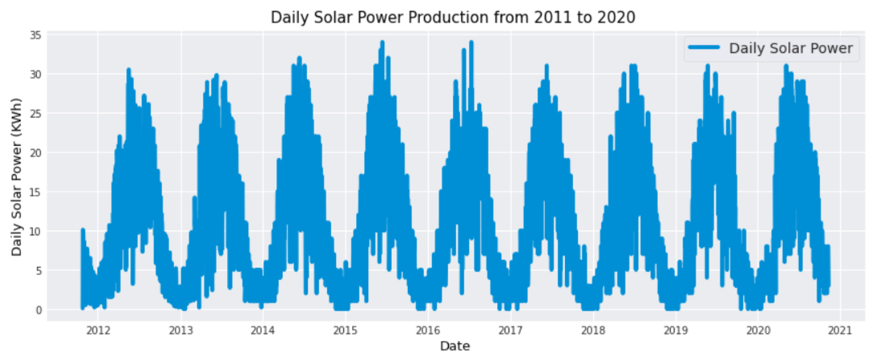
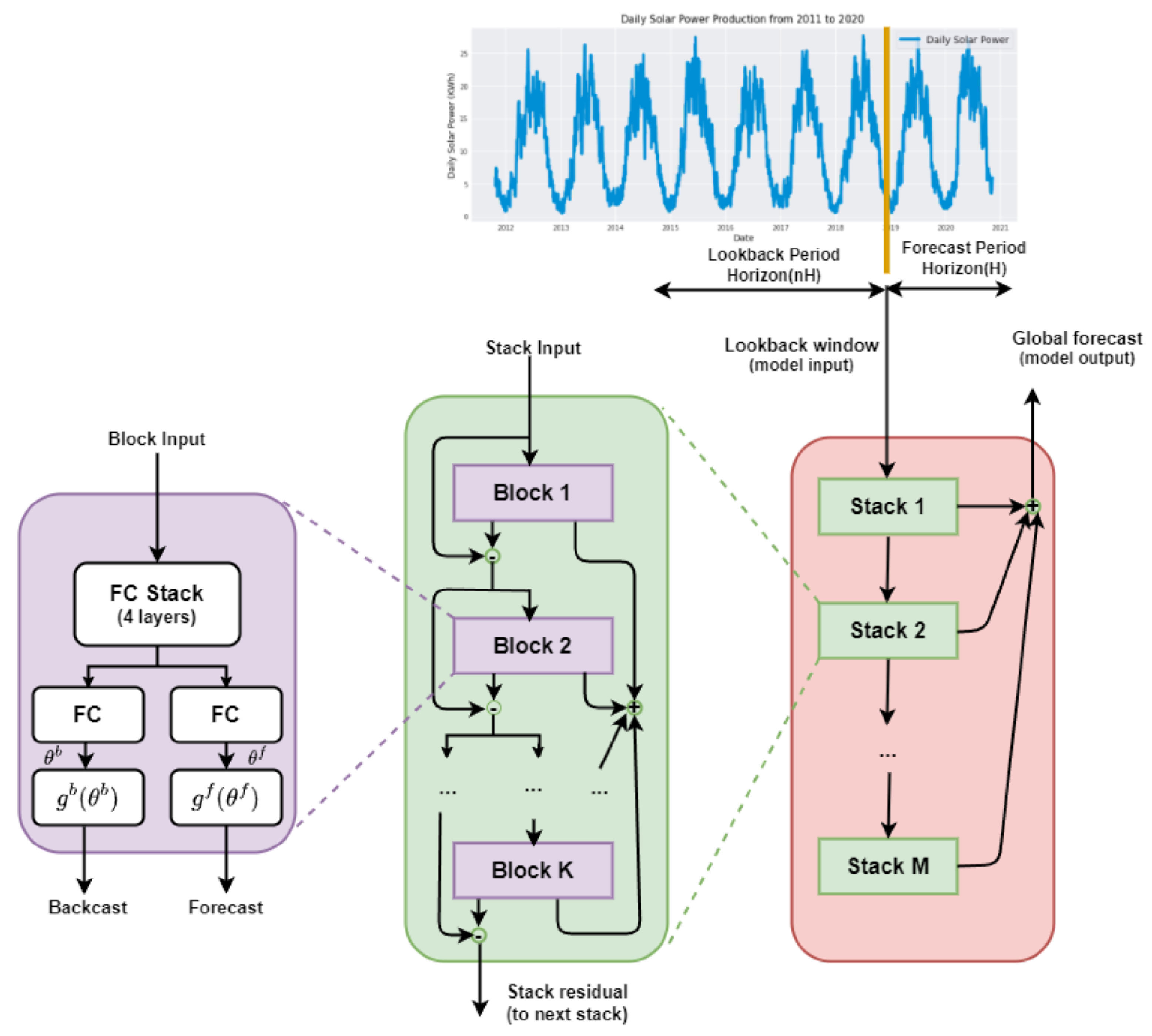
The daily solar power production distribution from 2011 to 2020 is graphically presented in Figure 1. It visually displays the trends, long-term patterns, and variations in solar power generation over this period.

Notably, as the data only provide cumulative values for solar energy produced, the study also computes the daily solar energy production and uses it as the target variable for the predictions.

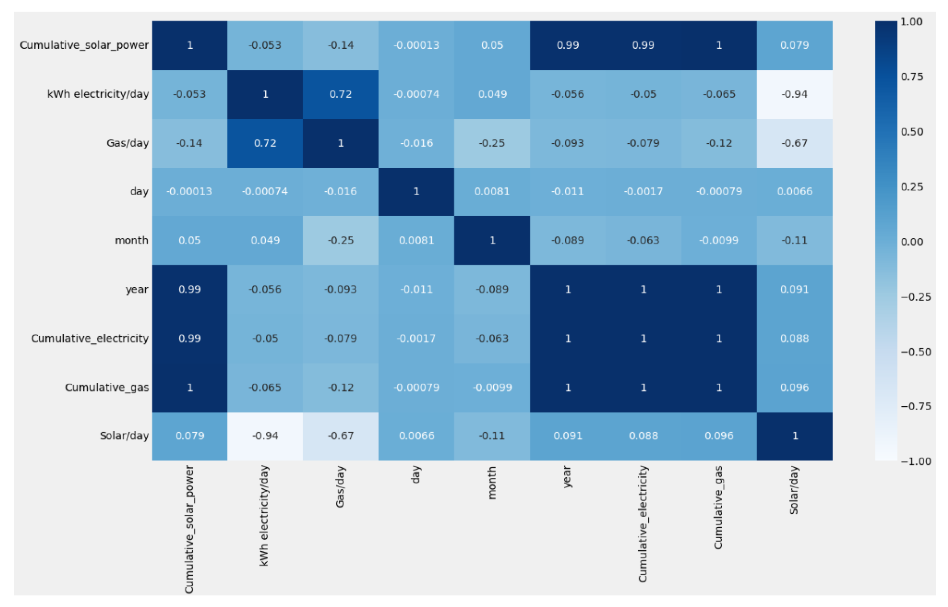
The correlation matrix measures the strength and direction of the relationship between two variables or series. Analyzing the correlation matrix makes it possible to determine which variables are most directly related to the target variable and how to utilize this information in the predictive model [27].

Figure 2 indicates positive correlations between the daily solar power production and cumulative_gas, cumulative_electricity, year, cumulative_solar_power, and day variables. However, there are no observed correlations between variables such as kWh electricity/day, gas/day, and month features in relation to daily solar power. This observation suggests that the variables that are positively correlated with daily solar power production may be good predictors, while variables that are not correlated may not be helpful in predicting daily solar power production.

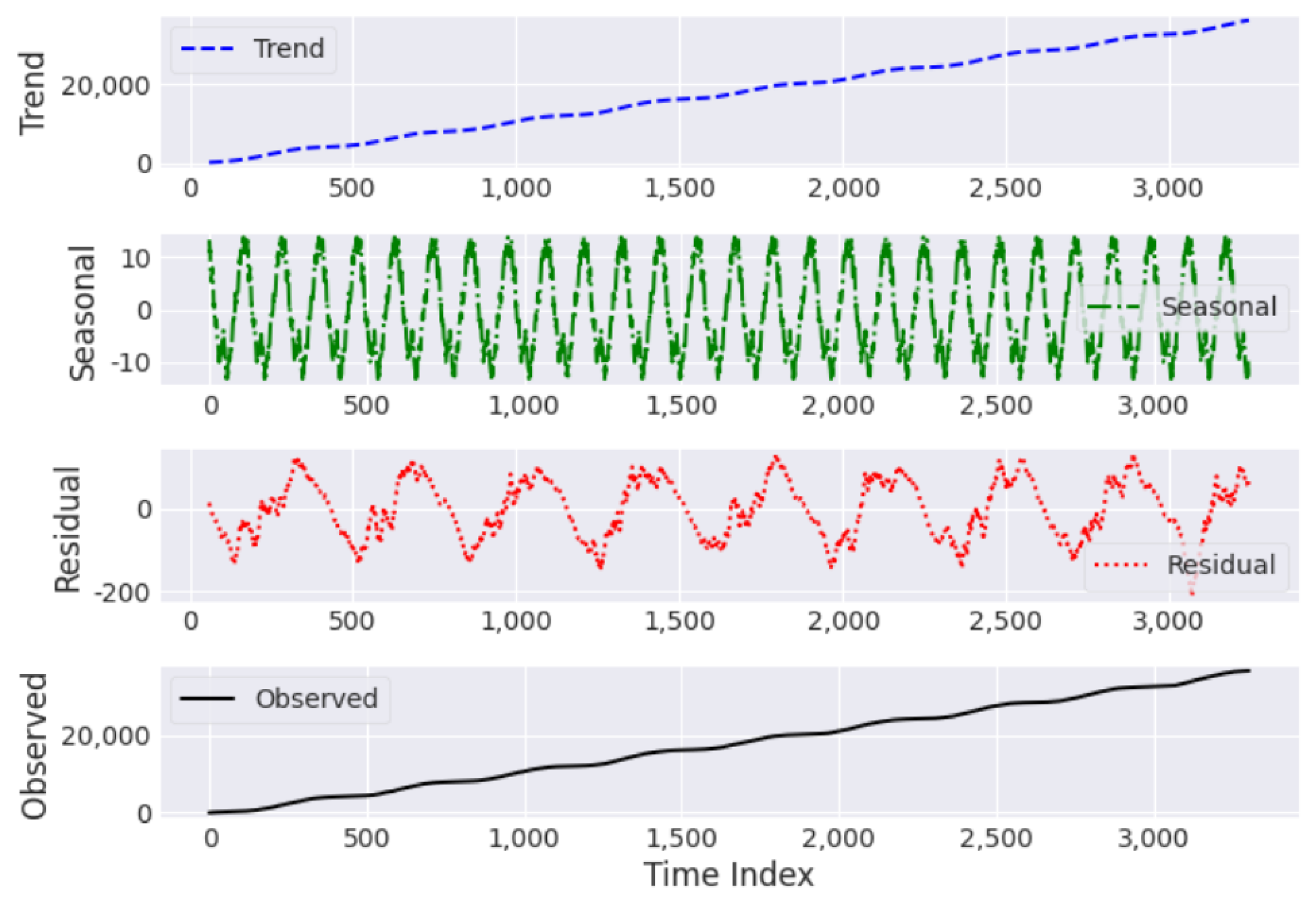
3.2.2. Seasonal Decomposition

Seasonal decomposition has been applied to the cumulative solar power time series to extract and analyze trends, seasonal patterns, and random fluctuations in the data. The additive decomposition method seems appropriate since the cumulative solar power data result from aggregating the daily production data. The additive decomposition technique analyzes the variation in the time series as the sum of the trend, seasonal, and residual components. Interpretation of this analysis can reveal that cumulative solar power demonstrates a uniform trend during seasonality and residual noise, as shown in Figure 3.

3.2.3. Triplet Exponential Smoothing

Exponential smoothing forecasting techniques share a common characteristic: a forecast is computed as a weighted summation of prior observations. However, these models are distinct in their utilization of exponentially declining weights for historical observations, wherein they incorporate explicit representations of underlying components, such as error, trend, and seasonality [28]. It involves three types, namely, simple exponential smoothing (SES), double exponential smoothing (DES), and triple exponential smoothing (TES). SES utilizes a smoothing parameter, ($\alpha$), to control the weightage of previous observations in the forecast. It is typically constrained to the interval [0, 1]. Under such a constraint, values approaching 1 indicate that the model assigns higher weight to more recent observations in representing the system’s dynamics, whereas values in proximity to 0 correspond to greater emphasis on historical data in forecasting future photovoltaic power output. In DES, an additional smoothing factor, ($\beta$), is introduced to accommodate the trend shift, while the TES or Holt–Winters seasonality method adds another smoothing factor, ($\gamma$), to deal with the impact of seasonality. The respective equations for level, trend, and seasonality in these three types of exponential smoothing are given by Equations (2)–(4) [29]:

$$l_t=\alpha y_t+\alpha (1-\alpha )y_{t-1}+\alpha {(1-\alpha )}^2{y}_{t-2}+\alpha {(1-\alpha )}^t{y}_0$$

(2)

where $l_t$ is used to represent the level of the time series at a specific timepoint t. Additionally, the individual observations within the series are denoted by the symbol $y_i$.

$$b_t=\beta (l_t-l_{t-1})+(1-\beta )b_{t-1}$$

(3)

At a specific time t, the equation for $b_t$ represents the trend component of the time series, while the equation for $l_t$ represents the level component.

$$s_t=\gamma (y_t-l_{t-1}-b_{t-1})+(1-\gamma )s_{t-m}$$

(4)

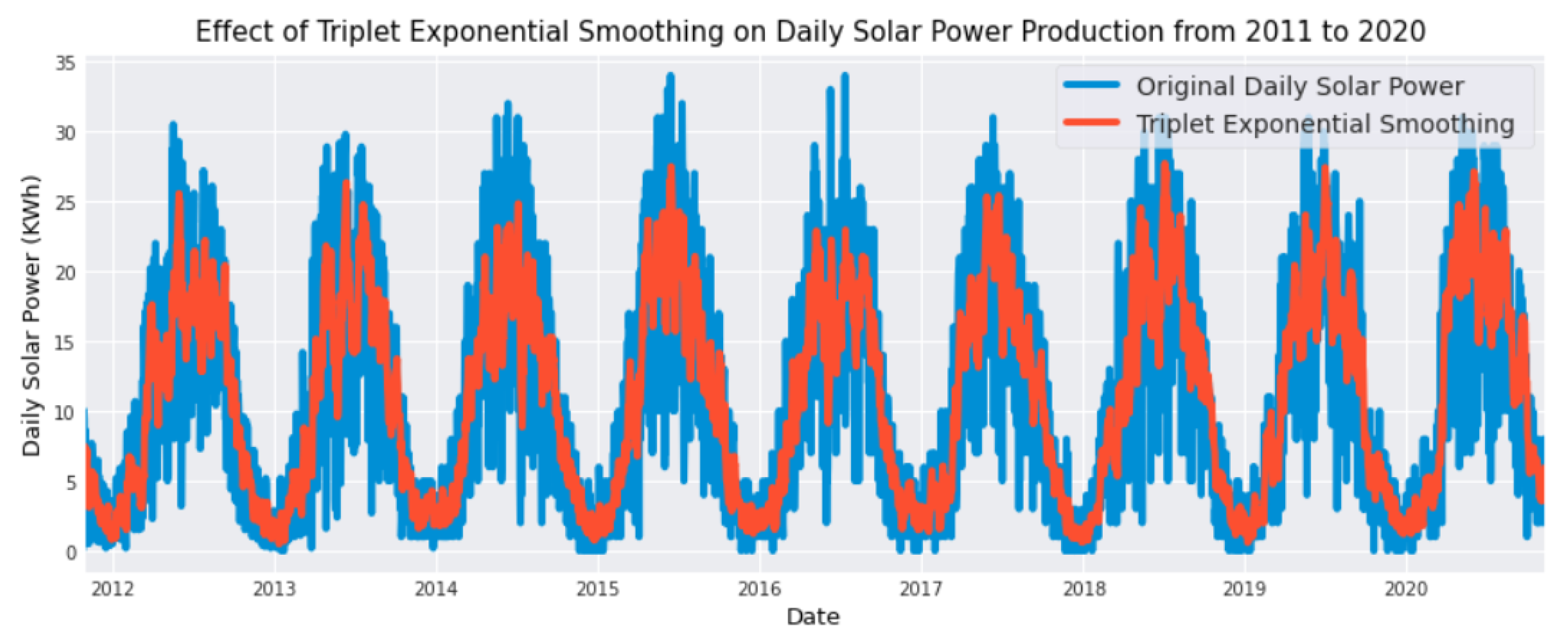
The term $(y_t-l_{t-1}-b_{t-1})$ denotes the current value of the seasonal component for the time series at time t. The seasonal equation calculates a weighted average of the current and historical seasonal indices that occurred m years prior. The application of triple exponential smoothing (TES) to daily solar power production time series is prompted by the effectiveness of this method in providing optimal forecast values for time series data characterized by both trend and seasonal patterns.

The results in Figure 4 indicate that utilizing TES on the daily solar power time series can produce values close to the actual data values.

3.3. Details about the Training Environment

The experimental setup for this study involved utilizing the Kaggle NVIDIA TESLA P100 GPU, CUDA11.1, Python3.8.8, and PyTorch1.11.0. An Adam optimizer was employed with a batch size of 64, and the training process consisted of 100 epochs. To implement the GRU-TFT, N-BEATS, NHiTS, and XGBoost models, we utilized the PyTorch Forecasting [30] software libraries that were made accessible for this purpose.

3.4. Temporal Fusion Transformer (TFT)

The temporal fusion transformer (TFT) model developed by the Google Cloud AI team is a deep learning model for high-performance multihorizon forecasting. It is an innovative neural network architecture that amalgamates LSTM layers, encoder–decoders, and attention heads from transformers. It consists of an encoder and decoder, where the former processes time series input and the latter generate context-aware embeddings for future value prediction. While LSTM modules capture short patterns, attention heads handle longer relationships, and a temporal multihead attention block prioritizes significant long-range patterns. The context vector passes through Gate and Add & Norm layers, while dropout mitigates overfitting during training. Gated layers control information flow within neurons, and self-attention aggregates data from different neurons, combining with residual connection weights in the Add & Norm layer. Layer normalization ensures consistent input across features, making TFT suitable for sequence models like transformers and recurrent neural networks.

The architecture of the TFT (transformer-based feature-wise transformation) model, as illustrated in Figure 5, exhibits the capability to proficiently generate feature representations for each input type through the utilization of canonical components. This feature engineering approach contributes to improved prediction performance across various prediction tasks. The primary components of TFT, as delineated below, encompass the following:

3.4.1. Gated Residual Network (GRN)

These mechanisms facilitate the exclusion of any unused components within the model by leveraging insights acquired from the data. Such adaptability bestows adaptive depth and network complexity, enabling the accommodation of diverse datasets. The integration of exponential linear unit (ELU) and gated linear unit (GLU) activation functions within the network serves the purpose of discerning input transformations of varying complexity. Notably, the resulting output undergoes standard layer normalization before final dissemination. The network architecture is enriched by a residual connection, affording the capability to adaptively attenuate input influence when deemed appropriate. The GRN comprises two distinct inputs: an optional context vector c and a principal input p, characterized by the following Equations (5)–(7):

$${\mathrm{GRN}}_w(p,c)=\&\mathrm{LayerNorm}(p+GL{U}_w\left({\eta }_1\right))$$

(5)

$${\eta }_1=\&W_{1,w}{\eta }_2+b_{1,w}$$

(6)

$${\eta }_2=\&ELU(W_{2,w}p+W_{3,w}c)b_{2,w}$$

(7)

In this context, ELU denotes the activation function, ${\eta }_1\in R^{d_{\mathrm{model}}},{\eta }_2\in R^{d_{\mathrm{model}}}$ represent intermediate layers, LayerNorm signifies standard layer normalization, and the subscript w signifies weight sharing. Noteworthy is the description of GLU as articulated below:

$${\mathrm{GLU}}_w\left(\gamma \right)=\sigma (W_{4,w}\gamma +b_{4,w})⨀(W_{5,w}\gamma +b_{5,w})$$

(8)

Here, the sigmoid activation function is represented as $\sigma$ for the input $\gamma$, while w and b denote weights and biases, respectively. The symbol ⨀ designates the element-wise Hadamard product. The architectural manipulation of the model through the generalized recurrent network is facilitated by the intricate functioning of GLU, which enables the potential disregard of additional layers. Importantly, GLU’s capacity to modulate nonlinear contributions by driving its outputs closer to zero offers the possibility of complete omission of this layer when exigencies dictate, as depicted in Figure 6.

3.4.2. Variable Selection Networks

In contrast to conventional deep neural networks (DNNs), attention-based variable selection within TFT aids in the identification of pertinent input variables at each time step. By enabling the removal of noise inputs, TFT can effectively eliminate irrelevant information that could potentially hinder its performance. This refinement process contributes to enhanced model accuracy and efficiency. This approach reduces the risk of overfitting irrelevant features and fosters enhanced generalization, as the model is encouraged to focus its learning capacity on the most salient features.

3.4.3. Static Covariate Encoders

TFT incorporates static features into the framework to govern the modeling of temporal dynamics. The consideration of static features can significantly impact forecasts; for instance, the temporal dynamics of sales may vary between different store locations, such as observing higher weekend traffic in rural stores and daily peaks after working hours in downtown stores. The static covariate encoders are strategically integrated into different layers of the model architecture, as depicted in Figure 5.

3.4.4. Temporal Processing

This facet of TFT encompasses acquiring both long- and short-term temporal dependencies from observed and known time-varying inputs. To achieve this, TFT utilizes a sequence-to-sequence layer for local processing, which benefits from its inductive bias in handling ordered information. Additionally, TFT employs a novel interpretable multihead attention block [31,32] to capture long-term dependencies. This innovative approach reduces the effective path length of information, allowing the model to directly focus on relevant information from past time steps.

3.4.5. Prediction Intervals

These intervals constitute quantile forecasts that ascertain the range of target values at each prediction horizon. By providing insights into the distribution of output rather than solely point forecasts, prediction intervals enhance users’ understanding of the uncertainty associated with the forecasts.

3.5. The DIstortion Loss Including Shape and TimE (DILATE) Loss

Dynamic time warping (DTW) is a method utilized to quantify the similarity between two time series by dynamically aligning the sequences, thereby effectively measuring the similarity between their respective variables. Distortion loss encompassing shape and time components (referred to as DILATE) constitutes an innovative objective function tailored for the training of deep neural networks in scenarios involving multistep and nonstationary time series forecasting. DILATE explicitly disentangles the penalization associated with shape discrepancies and temporal localization errors in the context of change detection.

The DILATE loss function, denoted as ${\mathcal{L}}_{\mathrm{DILATE}}(\mathbf{x},\mathbf{y})$, is defined as a linear combination of the shape loss function ${\mathcal{L}}_{\mathrm{shape}}(\mathbf{x},\mathbf{y})$ and the temporal loss function ${\mathcal{L}}_{\mathrm{temporal}}(\mathbf{x},\mathbf{y})$, modulated by the hyperparameter $\alpha \in [0,1]$. Here, $\mathbf{x}=\{x_1,\dots ,x_n\}$ represents the target sequence of length n, and $\mathbf{y}=\{y_1,\dots ,y_n\}$ symbolizes the predicted sequence of the same length n. It is given by Equation (9).

$${\mathcal{L}}_{\mathrm{DILATE}}(\mathbf{x},\mathbf{y})=\alpha ·{\mathcal{L}}_{\mathrm{shape}}(\mathbf{x},\mathbf{y})+(1-\alpha )·{\mathcal{L}}_{\mathrm{temporal}}(\mathbf{x},\mathbf{y})$$

(9)

A detailed description of ${\mathcal{L}}_{\mathrm{shape}}(\mathbf{x},\mathbf{y})$ and ${\mathcal{L}}_{\mathrm{temporal}}(\mathbf{x},\mathbf{y})$ is given in Equations (10)–(18).

The shape loss function is given by

$${\mathcal{L}}_{\mathrm{shape}}(\mathbf{x},\mathbf{y})={\mathrm{DTW}}_{\gamma }(\mathbf{x},\mathbf{y})$$

(10)

$${\mathrm{DTW}}_{\gamma }(\mathbf{x},\mathbf{y})=\underset{\mathbf{A}\in {\mathcal{A}}_{n,m}}{min}\left\{-\gamma log\left(\sum _{\mathbf{A}\in {\mathcal{A}}_{n,m}}{e}^{-\frac{\langle \mathbf{A},\Delta (\mathbf{x},\mathbf{y})\rangle }{\gamma }}\right)\right\}$$

(11)

$$\Delta (\mathbf{x},\mathbf{y})={\left[{\delta }_{i,j}\right]}_{n\times n}\in {\mathbb{R}}^{n\times n}$$

(12)

$$r_{i,j}={\delta }_{i,j}+min\left(\begin{array}{c}{r}_{i,j-1},r_{i-1,j},r_{i-1,j-1}\end{array}\right)$$

(13)

$$mi{n}_{\gamma }\{a_1,\dots ,a_n\}=\left\{\begin{array}{cc}\underset{i\le n}{min}{a}_i\hfill & ,\mathrm{if}\gamma =0\hfill \\ -\gamma log\sum _{i=1}^n{e}^{-a_i/\gamma }\hfill & ,\mathrm{if}\gamma >0\hfill \end{array}\right)$$

(14)

$$r_{n,n}={\mathrm{DTW}}_{\gamma }(\mathbf{x},\mathbf{y})$$

(15)

where ${\mathcal{A}}_{n,m}\subset {\{0,1\}}^{n\times n}$ is the set of calibration matrices for two sequences of lengths n and m, representing all possible paths from $(x_1,y_1)$ to $(x_n,y_m)$. $\mathbf{A}$ represents a path in ${\mathcal{A}}_{n,m}$. $\Delta (\mathbf{x},\mathbf{y})$ is the cost matrix composed of pairwise costs, and ${\delta }_{i,j}$ denotes the corresponding cost. $\gamma$ is a hyperparameter controlling the optimal paths. Equations (13) and (14) define the “optimal” paths for solving the two sequences, with $\gamma$ affecting the solution process differentiability.

The temporal loss function is defined as

$${\mathcal{L}}_{\mathrm{temporal}}(\mathbf{x},\mathbf{y})\&=\langle {\mathbf{A}}^{*},\Omega \rangle$$

(16)

$$\Omega \&={\left[w_{i,j}\right]}_{n\times n}\in {\mathbb{R}}^{n\times n}$$

(17)

$$w_{i,j}\&=\frac{1}{n^2{(i-j)}^2}$$

(18)

Here, $\Omega$ is a square matrix penalizing associations between elements of $\mathbf{x}$ and $\mathbf{y}$, especially when the indices i and j significantly deviate. ${\mathbf{A}}^{*}$ is the “optima” path obtained from the computation of ${\mathrm{DTW}}_{\gamma }(\mathbf{x},\mathbf{y})$. The goal of ${\mathcal{L}}_{\mathrm{temporal}}(\mathbf{x},\mathbf{y})$ is to penalize excessive temporal lags during the DTW process.

3.6. Neural Basis Expansion Analysis for Interpretable Time Series Forecasting (N-BEATS)

The N-BEATS architecture [33] represents a departure from traditional RNN methodologies for sequence forecasting. Instead of processing timepoints sequentially, N-BEATS adopts a holistic approach by considering an entire window of past values and generating multiple forecast timepoints in a single pass. This is facilitated through the extensive utilization of fully connected layers to forecast the trend and seasonality components. As delineated by the formulation in Equation (19) [33], the trend model is subjected to a constraint wherein it adheres to a polynomial function of a modest degree p, embodying a gradual variation across the forecast window. The resultant prediction, $y_b$, is expressed as the summation over a polynomial expansion:

$$y_b=\sum _{i=0}^p{\theta }_{tr,it}·t^i$$

(19)

In this context, the temporal vector t is defined as $t={[0,1,2,\dots ,H-2,H-1]}^T/H$, discretely spanning the interval from 0 to $(H-1)/H$. The prediction for H time steps ahead, $y_b$, is determined by the polynomial coefficients ${\theta }_{tr}$, which are anticipated through the agency of a fully connected network.

Analogously, the seasonality model, elucidating recurring cyclic patterns, is subject to the constraint of the Fourier basis, as embodied by Equation (20) [33]. In this context, $y_b$ is expressed as a linear combination of Fourier basis functions:

$$y_b=\sum _{i=0}^{⌊\frac{H}{2}⌋-1}{\theta }_{sea,i}cos\left(2\pi it\right)+{\theta }_{sea,i+⌊\frac{H}{2}⌋}sin\left(2\pi it\right)$$

(20)

Here, the Fourier coefficients ${\theta }_{sea}$ are prognosticated by a fully connected network, encapsulating the cyclic and repetitive fluctuations inherent in the seasonality model. This architecture effectively captures the complex temporal patterns present in the time series data, facilitating an interpretative framework for forecasting PV solar power generation. The architecture is composed of multiple interconnected blocks that employ a residual framework. The initial block endeavors to accurately model both the past window (backcast) and the future (forecast). Subsequent blocks focus on capturing the residual error of the previous block’s reconstruction and updating the forecast accordingly. The residual design enables the stacking of numerous blocks without the risk of gradient vanishing. Moreover, it incorporates the principles of boosting/ensembling techniques prevalent in classical machine learning, where the forecast is a summation of predictions from multiple blocks. Each block specializes in capturing distinct elements, with the first block capturing overarching trends and subsequent blocks dedicated to addressing smaller errors.

Furthermore, the N-BEATS architecture accommodates specialized trend and frequential blocks. These blocks acquire the parameters of specific functions, such as polynomial trends and sinusoidal/cosinusoidal functions with varying frequencies.

N-BEATS offers several notable advantages over traditional approaches:

• Accelerated training: The parallelization of operations on GPUs enables faster training compared with recurrent networks.
• Lightweight networks: The flexible configuration of N-BEATS blocks enables the design of more lightweight networks.
• Customizable backcast and forecast: N-BEATS can adapt to incorporate arbitrarily long past sequences and forecast into the future. The model configuration is adjusted accordingly based on the specific requirements of the forecasting task.

In summary, the N-BEATS architecture presents an alternative paradigm for sequence forecasting, leveraging the extensive use of fully connected layers and a residual framework. This approach offers expedited training, lightweight network structures, and the flexibility to tailor the backcast and forecast capabilities to the specific demands of the problem at hand. The N-Beats design has a hierarchical structure, with crucial components being a series of nested stacks, each of which is made up of numerous fundamental blocks. The intricate architectural configuration is vividly illustrated in Figure 6, providing a comprehensive visual representation of its organizational intricacies.

3.7. Neural Hierarchical Interpolation for Time Series Forecasting (NHiTS)

Neural hierarchical interpolation for time series forecasting (NHiTS) is an advanced methodology designed for improving the accuracy and efficiency of time series forecasting. Developed by Challu et al. [34], NHiTS builds upon the foundational N-BEATS framework introduced by Oreshkin and his colleagues in 2020.

The core innovation of NHiTS involves a hierarchical approach to forecasting, combining multirate sampling techniques and multiscale synthesis strategies. This hierarchical construction not only reduces computational demands but also enhances the precision of long-term forecasts.

Similar to its precursor N-BEATS, NHiTS employs local nonlinear mappings onto fundamental basis functions across various blocks. Each block is equipped with an MLP responsible for computing coefficients for both backcasting and forecasting tasks related to its underlying basis. The backcast output refines subsequent input, while the aggregate forecast outputs yield the final predictive outcome. These blocks are grouped into stacks, each specialized in capturing distinct data attributes through unique sets of basis functions. The input to NHiTS denoted as $y_{t-L:t}$ encapsulates historical lags up to a specified count “L”.

NHiTS comprises multiple stacks, with each stack housing numerous blocks. Within each block, MLP undertakes the prediction of forward and backward basis coefficients, facilitating an intertwined information flow across time. The architecture introduces novel components to enhance the predictive capabilities of the model.

In summary, NHiTS represents a novel and sophisticated framework for time series forecasting, leveraging a hierarchical approach, multirate sampling, and multiscale synthesis to achieve higher forecasting accuracy and computational efficiency. The collaborative efforts of its developers have resulted in a promising advancement in the field of time series analysis.

4. Results

In this section, the presented model undergoes comprehensive testing, and its performance is subjected to thorough analysis through the lens of various evaluation metrics. Subsequent to this assessment, a comparative evaluation is conducted, wherein the model’s performance is evaluated against that of cutting-edge models and contemporary investigations executed on the identical dataset.

Evaluation Metrics

In this work, we utilize four metrics to assess the models: MAE, MSE, and RMSE. They are given by Equations (21)–(23):

$$\mathrm{MAE}=\frac{1}{N}\sum _{i=1}^N|y_i-\widehat{y}|$$

(21)

$$\mathrm{MSE}=\frac{1}{N}\sum _{i=1}^N{(y_i-\widehat{y})}^2$$

(22)

$$\mathrm{RMSE}=\sqrt{\frac{1}{N}\sum _{i=1}^N{(y_i-\widehat{y})}^2}$$

(23)

where N denotes the number of rows in the dataset, $y^i$ denotes the actual values of the solar power, and $\widehat{y}$ is the forecasted values of the solar power MAE, which, being a common evaluation metric, does not consider the direction of prediction errors and solely focuses on measuring the average magnitude of these errors. Specifically, it quantifies the average absolute difference between the model’s predictions and the corresponding actual values across the entire testing dataset. RMSE is a metric used to assess the spread or dispersion of residuals in a predictive model. It calculates the standard deviation of prediction errors, providing a measure of how closely the model’s predictions align with the actual observed values. By taking the square root of the mean of squared errors, RMSE accounts for both the magnitude and direction of prediction errors, yielding a comprehensive evaluation of the model’s overall performance. A lower RMSE value indicates that the model’s predictions are more accurate and have a smaller spread around the true values, while a higher RMSE value signifies greater variability and potential inaccuracies in the model’s predictions. MSE is an assessment statistic that measures the average difference between expected and actual values [35]. The mean of the squared discrepancies between each forecast and its matching true value is used to calculate it. The average of the squared differences is then calculated to establish the overall average error between the model’s predictions and the observed values. To demonstrate the superiority of the proposed model, we have performed the two-sided Diebold–Mariano test [36]. In hypothesis testing, a two-sided test considers both directions of the alternative hypothesis, while a one-sided test focuses on only one direction. In the context of the Diebold–Mariano test, a two-sided test allows for the detection of differences in both positive and negative directions between the forecast errors of two models. It compares the null hypothesis that the forecast errors are equal against the alternative hypothesis that the forecast errors are different in either direction. By using a two-sided test, the possibility of differences in both positive and negative directions is examined, providing a more comprehensive analysis of the forecast errors.

5. Discussion

Table 1. Effect of increasing the number of attention heads with an LSTM encoder/decoder.

	MAE		MSE		RMSE
	MSE	DILATE	MSE	DILATE	MSE	DILATE
2 Attention Heads	1.6	1.26	3.3	2.34	1.81	1.53
4 Attention Heads	1.24	1.24	2.24	2.24	1.49	1.49
8 Attention Heads	1.37	1.38	2.57	2.9	1.6	1.7

and

Table 2. Effect of increasing the number of attention heads with a GRU encoder/decoder.

	MAE		MSE		RMSE
	MSE	DILATE	MSE	DILATE	MSE	DILATE
2 Attention Heads	1.6	1.26	3.3	2.34	1.81	1.53
4 Attention Heads	1.32	1.19	2.46	2.08	1.57	1.44
8 Attention Heads	1.36	1.38	2.53	2.9	1.6	1.7

present a comprehensive overview of the impact of increasing the number of attention heads within the context of LSTM encoder/decoder and GRU encoder/decoder frameworks, respectively. As shown in Table 1, the findings reveal that when utilizing two attention heads in conjunction with an LSTM encoder/decoder, the DILATE loss function and the MSE loss function exhibit the same performance in terms of MAE, MSE, and RMSE. It is notable that both loss functions exhibit improved performance in terms of MAE, MSE, and RMSE when the LSTM encoder/decoder is replaced with its GRU counterpart as demonstrated in Table 2.

Upon increasing the number of attention heads to four, both loss functions produce similar results when using the LSTM architecture. It is worth noting that both loss functions demonstrate improved performance in terms of MAE, MSE, and RMSE when the LSTM encoder/decoder is replaced with the GRU counterpart. The highest performance was achieved when employing the GRU architecture in conjunction with the DILATE loss function. The MAE, MSE, and RMSE values for the GRU/DILATE architecture have been reduced to 1.19, 2.08, and 1.44, respectively, as shown in Table 2.

Raising the number of attention heads to eight results in a considerable drop in performance. The rise in MAE, MSE, and RMSE demonstrates this. For LSTM and GRU encoder/decoder models using the DILATE loss function, the values are 1.38, 2.9, and 1.7, respectively. On the other hand, when the MSE loss function is used for the GRU encoder/decoder, the MAE, MSE, and RMSE values increase to 1.36, 2.53, and 1.6, respectively. Furthermore, for the LSTM encoder/decoder with the MSE loss function, the respective values rise to 1.37, 2.57, and 1.6.

These results indicate that employing eight attention heads with either an LSTM encoder/decoder or a GRU encoder/decoder, along with the DILATE or MSE loss function, leads to inferior performance in terms of MAE, MSE, and RMSE when compared with other configurations.

A detailed inspection of Table 1 and Table 2 demonstrates the negative impact of increasing the number of attention heads to eight regardless of the loss function used.The TFT model utilizes multiple attention heads to capture different patterns and dependencies in the data. The use of different numbers of attention heads allows the model to focus on various aspects of the input sequence, enhancing its ability to capture complex patterns and potentially improve forecasting accuracy. However, the impact of different numbers of attention heads on accuracy can vary depending on the dataset and task, and experimentation is necessary to determine the optimal configuration. Through a thorough analysis of the obtained outcomes, several salient conclusions can be drawn:

• DILATE loss has a tendency to outperform MSE loss when combined with the GRU encoder/decoder, although this trend is subject to variabilities contingent on hyperparameters, notably the number of attention heads.
• The substitution of the LSTM encoder/decoder with its GRU counterpart improves overall performance, irrespective of the selected loss function MSE or DILATE, which constitutes the principal contribution of the proposed methodology.
• It is noteworthy that DILATE loss is characterized by a higher temporal complexity in comparison with MSE loss.

To ascertain the most suitable hyperparameters for the proposed GRU-TFT model, we engage in a thorough process of hyperparameter tuning, wherein pivotal hyperparameters are systematically adjusted. Initially, the focal point lies in the network’s “hidden_size,” a principal hyperparameter denoting the extent of neural activity within each dense layer of the GRN. The range of exploration spans from 8 to 512. Subsequently, attention turns to the “hidden_continuous_size” parameter, which signifies the magnitude of neurons inhabiting each dense layer within the continuous segment of the network [37]. To ensure coherence, it is advisable that this parameter assumes a value equivalent to or lesser than “hidden_size”; hence, for alignment, it is aligned with “hidden_size.” The “dropout” parameter governs the extent of dropout integration within TFT layers in which dropout mechanisms operate. Meanwhile, the ”learning rate” is meticulously fine-tuned over a continuum ranging from 0.0001 to 0.1. Lastly, we undertake the calibration of the “number of attention heads,” spanning from 1 to 8.

The upshot of this hyperparameter exploration endeavor is encapsulated within

Table 3. Hyperparameter configurations for the temporal fusion transformer model.

Hyperparameter	Value
attention_head_size	4
Lstm/gru_layers	2
hidden_size	100
hidden_continuous_size	100
learning_rate	1 × 10${}^{-4}$
dropout	0.1
alpha(DILATE loss)	0.9
gamma(DILATE loss)	0.01

. The exploration encompasses a spectrum of configurations, culminating in the identification of the hyperparameters that optimally suit our specific dataset and the exigencies of the forecasting task. Specifically, the optimal parameter configuration materializes as 100 for “hidden_size,” 100 for “hidden_continuous_size,” and a learning rate of 0.0001, accompanied by four attention heads. This constellation of hyperparameters significantly outperforms alternative configurations in the context of the loss function. Notably, the model MAE registers at 1.19, while MSE and RMSE stand at 2.08 and 1.44, respectively.

The primary aim of this study was to assess the efficacy of the TFT model in predicting energy consumption patterns using a specific dataset. The evaluation of the TFT model’s effectiveness involved a comparative analysis with two prominent methods for time series forecasting: N-BEATS [33] and NHiTS [34]. By identifying the optimal configuration of hyperparameters for the TFT model, we proceeded to contrast its predictive performance against two benchmark models, namely, N-BEATS and NHiTS, in the context of energy consumption forecasting. The hyperparameter settings of the N-BEATS model are presented in

Table 4. Hyperparameter configurations for the N-BEATS model.

Hyperparameter	Value
Stack_types	[‘seasonality’, ‘generic’]
num_blocks	[3, 3]
num_block_layers	[4, 4]
widths	[256, 512]
dropout	0.1
learning_rate	1 × 10${}^{-4}$

.

To facilitate the activation of the interpretable mode, the configuration of “stack_types” has been established to [’seasonality’, ’generic’]. The parameter “num_blocks” pertains to the count of blocks present within each stack, whereas “num_block_layers” denotes the quantity of fully connected layers featuring ReLu activation within each individual block. In accordance with the guidelines for facilitating interpretability, the values of “num_blocks” and “num_block_layers” have been designated as 3 and 4, respectively.

The hyperparameter denoted as “widths” corresponds to the dimensional extents of the fully connected layers incorporating ReLu activation situated within the blocks. While it is advisable for the interpretable mode to adopt dimensions [256, 2048], empirical findings indicate that superior outcomes are attainable with dimensions [256, 512].

To ensure an equitable comparison, the same dataset and learning rate values were utilized for each model. The findings resulting from this comparison between the TFT model, N-BEATS, NHiTS, and XGBoost are presented in

Table 5. Comparison of model performance in terms of MAE, MSE, and RMSE for the proposed GRU-TFT model, and other recent models.

Model	MAE	MSE	RMSE
GRU-DILATE-TFT [ours]	1.19	2.08	1.44
N-BEATS	1.997	6.729	2.594
NHiTS	2.622	9.029	3.005
XGBoost	9.691	149.981	12.246
Holt-Winters [29]	4.126	29.105	5.394
AR model [29]	7.194	77.590	8.808
ARIMA [29]	11.471	206.442	14.368
SARIMAX [29]	10.907	192.361	13.869

. In contrast with the deep learning models, the XGBoost model demonstrated the most suboptimal performance.

The empirical outcomes demonstrated that the TFT model exhibited superior predictive performance when compared with the N-BEATS model, showing an MAE, MSE, and RMSE of 1.997, 6.729, and 2.594, respectively, as well as the NHiTS model, registering an MAE, MSE, and RMSE of 2.622, 9.029, and 3.005, respectively. 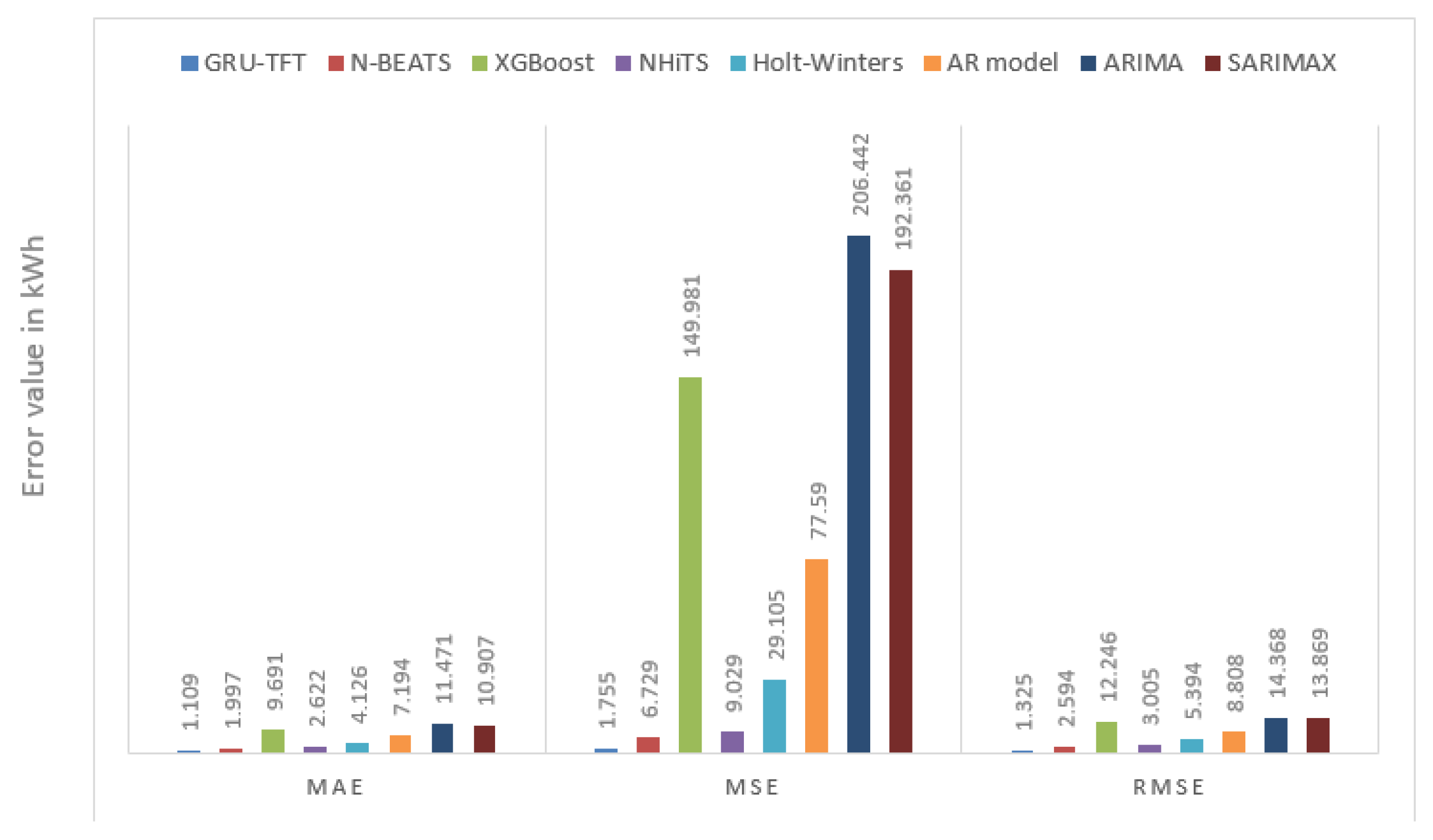It is of significance to highlight that the novel GRU-TFT model, which we have introduced, has demonstrated superior performance compared with the forecasting methodologies presented [29] encompassing the Holt–Winters AR, ARIMA, and SARIMAX models. While the Holt–Winters method for time series forecasting in the additive mode yields predictions proximate to the empirical values of solar power, exhibiting an RMSE metric of 5.3949, the newly introduced GRU-TFT model demonstrates a significantly enhanced performance when combined with the DILATE loss with an achieved RMSE score of 1.44. This remarkable improvement underscores the superiority of the GRU-TFT model in the domain of solar power prediction. The results presented in Table 5 are graphically illustrated within Figure 7.

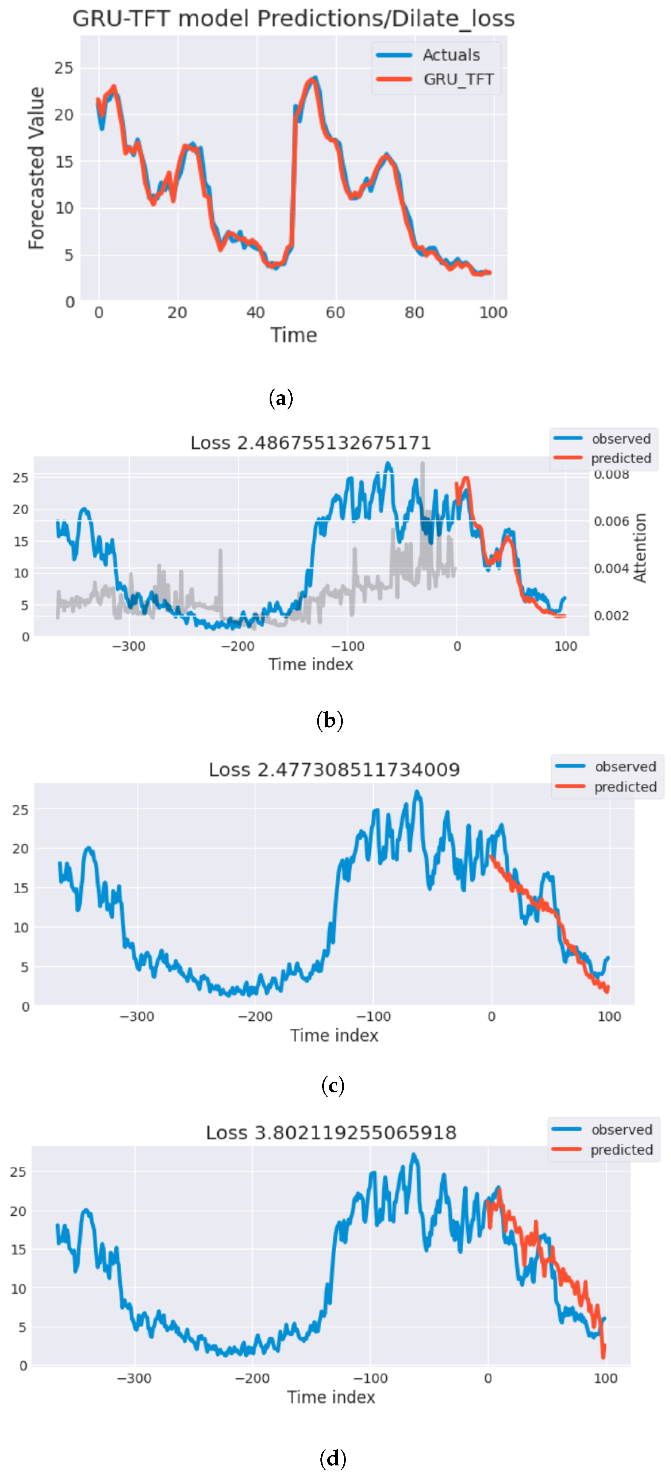
The lack of sensitivity of the MSE loss function to temporal information can result in delays in time series forecasting. These delays can lead to discrepancies between the predicted and actual load conditions, which can negatively impact the performance of PV cells. To address this issue, a new loss function known as DILATE is proposed. Shape error and temporal distortion are used as loss variables in the DILATE loss function, minimizing the impacts of temporal offset and distortion. As a result, the model can catch and account for such temporal information, yielding a more accurate prediction. Comparative studies were performed utilizing both the MSE and DILATE loss functions to examine the effectiveness of the DILATE loss function. Figure 8 depicts the projected results of the proposed model using DILATE and MSE loss functions, N-BEATS, and NHiTS in kWh in proportion to the observed energy values. The results show that the GRU-TFT model with DILATE loss (Figure 8a) beats the GRU-TFT model with MSE loss (Figure 8b) in terms of prediction accuracy. 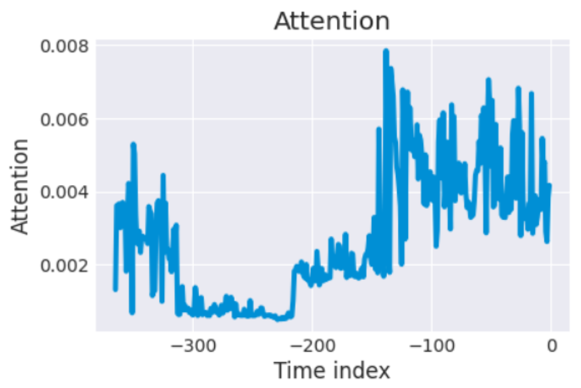The loss value shown at the top of Figure 8b corresponds to the MSE loss, whereas the loss value shown in the curves of N-BEATS (Figure 8c) and NHiTS (Figure 8d) represents the mean absolute scaled error (MASE) loss function. The proposed GRU-TFT model employs its innovative interpretable multihead attention mechanism to quantify the significance of preceding time steps. By investigating the attention weights, TFT aims to discern temporal patterns manifested throughout past time steps. As shown in Figure 9, the attention scores are represented by the blue lines, revealing the relative impact of these time steps on the model’s predictions. Minor peaks in the attention scores indicate daily seasonality, while a prominent peak towards the latter portion of the plot suggests the presence of weekly seasonality. Utilizing attention weight patterns, one can gain insights into the critical past time steps upon which the TFT model bases its decision-making process. This is in stark contrast with conventional time series methodologies in both traditional and machine learning domains, which heavily rely on model-driven specifications to analyze seasonality and lag phenomena. The TFT model, on the other hand, possesses the ability to autonomously learn and extract such patterns directly from the raw training data.

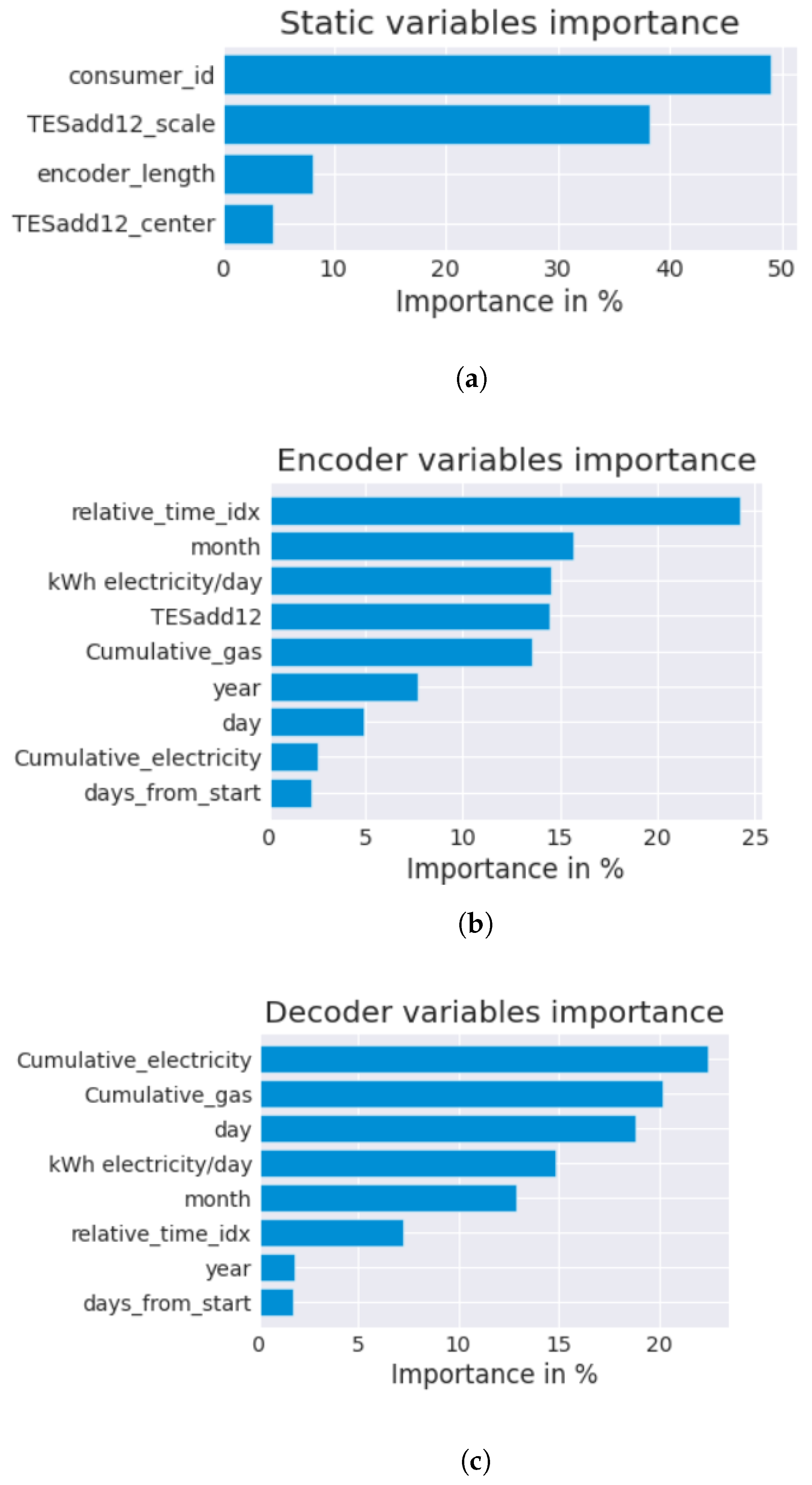
The architectural design of the TFT model incorporates inherent interpretive capabilities. It harnesses its variable selection network module to assess the significance of each feature as depicted in Figure 10. These graphical representations enable the visualization and comprehension of the relative importance of different features in forecasting the output of photovoltaic solar power where TESadd12 represents the daily solar power production time series after being preprocessed by the Holt–Winters method in additive mode, as well as TES. After conducting a two-sided Diebold–Mariano test to compare the performance of the proposed GRU-DILATE-TFT model against those of the XGBoost, NHiTS, and N-BEATS models, the resulting p-values were calculated as 1.3110 × 10${}^{-20}$, 2.0144 × 10${}^{-9}$, and 1.8117 × 10${}^{-6}$, respectively. Given that these p-values are all less than the significance level of 0.05, it can be inferred that there exists a statistically significant difference in accuracy between the proposed GRU-DILATE-TFT model and the other models examined.

6. Conclusions

This paper introduces a novel approach termed the GRU-TFT model, wherein the traditional LSTM encoder–decoder architecture is substituted with a GRU encoder–decoder arrangement. Furthermore, an augmented loss function termed “DILATE” is introduced, which incorporates shape and temporal distortion principles rooted in dynamic time warping as a means to address the prediction latency issue arising from the usage of the MSE loss function. This inclusion serves the purpose of providing instructive guidance to the model, aligning its training trajectory towards the enhancement of sequence similarity. To identify the pivotal variables for the model, an assessment of the significance of both the decoder and encoder variables was conducted. A comparative analysis was performed between the GRU-TFT model proposed in this study and two well-established methods for time series forecasting, namely, N-BEATS and NHiTS. Holt–Winters additive forecasting approximates solar power values with RMSE 5.3949. In contrast, the new GRU-TFT model achieves an RMSE of 1.44, demonstrating remarkable superiority for solar power prediction. Furthermore, experiments show that the suggested GRU-TFT model always outperforms six well-used techniques in the context of time series computational tasks. This research provides an adaptable approach that can be applied to a variety of forecasting issues. This methodology shows promise for increased performance when adapted to the features of the dataset under consideration. The suggested GRU-DILATE-TFT model performs much better in the Diebold–Mariano test than the XGBoost, NHiTS, and N-BEATS models, as evidenced by p-values less than 0.05. One possible future study direction is to use a combination of TFT and graph neural networks for forecasting the output of PV solar power generation. This method relies on the spatial correlation acquired by the graph neural network. Furthermore, including external parameters such as weather forecasts, market pricing, and grid conditions in deep learning models for PV forecasting could improve prediction accuracy and reliability. This can include creating hybrid models that incorporate deep learning and other forecasting techniques, as well as using external data as extra input features. Extending deep learning models to allow for real-time or intraday PV forecasting could be an attractive future research path. This would include creating models capable of dealing with high-frequency data and providing accurate and timely forecasts over shorter time horizons. Ensemble methods, such as combining multiple deep learning models or integrating deep learning with traditional statistical models, can be investigated to improve the accuracy and robustness of day-ahead PV forecasting. Ensemble techniques can help mitigate the inherent uncertainty and variability in PV power generation.