Abstract
A detailed description of wake characteristics is essential for optimizing wind farm performance. Compared with the wake of a stand-alone wind turbine, less attention has been paid to wind turbine wakes in large wind farms. In this work, we investigate the vertical position of wakes for wind turbines in large wind farms with different streamwise turbine spacings and ground roughness lengths using large-eddy simulation with an actuator disk model. The simulation results reveal an upward shift of the wake center (defined as the position with the maximum velocity deficit) for the wind turbine deeply arrayed in the wind farm. Larger upward shifts of the wake center are observed for wind turbines in further downstream rows and wind turbines installed on the ground with higher roughness, for which the wake expands at a higher rate. It is conjectured that the upward shift of the wake center is caused by the upward shift of the turbulence-dominated momentum entrainment region and the constraint of ground on wake expansion. An analytical wake model incorporating the upward-shifting wake center was developed. In the proposed model, different expansion rates are employed for the lower and upper wake regions. The upward shift of the wake center is directly taken into account using the large-eddy simulation results. The comparison with the large-eddy simulation results demonstrates the importance of accounting for the upward shift of the wake center in analytical wake models.
1. Introduction
Wind turbine wakes affect both power generation across wind farms and fatigue loads on turbine structures [1,2]. Accurately describing the spatial distribution of velocity deficits in wind turbine wakes is important for mitigating their negative impacts. In this work, we numerically characterize the vertical position of turbine wakes in large wind farms, analyze the underlying mechanisms, and demonstrate the importance of accounting for vertical wake position changes in analytical wake models.
The ground surface and atmospheric boundary layer inflow represent the two key factors influencing the vertical distribution of wake statistics. The ground impedes wake expansion toward the surface. The vertical variations in wind speed and turbulence intensity of the inflow affect momentum entrainment from both the top region of the wake and the region beneath the wake. As shown in wind tunnel experiments and numerical simulations of a stand-alone wind turbine [3,4,5], the vertical distribution of streamwise velocity deficit is symmetrical about hub height at near and intermediate wake locations (e.g., and (D is rotor diameter)) while becoming asymmetrical at further wake locations. Experiments by Chamorro and Porte-Agel [3] also showed that at far wake locations, the region above hub height is wider than that below hub height. Regarding turbulence intensity, it is higher around the top tip of the turbine compared to the bottom tip at intermediate wake locations (e.g., ), with this difference becoming less pronounced at further wake locations (e.g., ) [3,6].
Analytical wake models are crucial for designing wind farm layouts and optimizing wind farm controls [2,7]. Most analytical models [8,9,10,11] compute velocity deficit using a single-wake expansion rate, assuming a symmetric vertical distribution about the hub height without accounting for the influences from the atmospheric inflow or the ground. In the pioneering work by Lissaman [12], approaches to account for the ground and nonuniform inflow effects were suggested: (1) modeling the retarding effect of the ground on wake expansion using an imaging technique; (2) assuming the streamwise deficit distribution for the boundary layer inflow being identical to the uniform inflow; and (3) employing distinct upper and lower wake expansion rates to account for the vertical variation of turbulence intensity. Recent analytical wake models have employed approaches similar to those suggested by Lissaman to account for the atmospheric inflow effects [13,14,15].
On wind farms, wake interference has often been modeled using superposition rules [16,17,18,19], such as linear superposition of velocity deficits [12,20] or squares of velocity deficits [21,22]. In addition to wake superposition, turbulence from upstream wakes also influences the downwind wake development. Studies showed that wakes are wider for a waked wind turbine compared with those facing undisturbed winds [23]. Moreover, an upward shift in the wake center is observed for turbines deep within arrays in wind tunnel experiments [24] and in the large-eddy simulation of a very long wind turbine wake [25].
However, the upward shifts in turbine wake centers have not been systematically studied or incorporated into analytical models. Characterizing and modeling such upward shifts is important for accurate computation of wind turbine power and structure load as well as wake steering in the vertical direction using tilt control [26]. In this work, we investigate the upward shift of the wake center for wind turbines in wind farms with various streamwise wind turbine spacings and ground roughness lengths using large-eddy simulation (LES) and test how the upward shift affects the prediction accuracy of analytical wake models. The novelty of this work lies in the systematic examination of the upward shift of the wake center in large wind farms and the development of an analytical wake model to account for its effect on the vertical distribution of velocity deficit.
The rest of the paper is organized as follows. First, the employed LES method is described in Section 2. Then, the case setup is given in Section 3. The analyses of the simulation results and the test of analytical wake models are carried out in Section 4. Lastly, the conclusions are drawn in Section 5.
2. Numerical Method
Simulations of wind turbine wakes are conducted using large-eddy simulation (LES) utilizing an actuator disk model for wind turbine aerodynamics. The LES module of the VFS-Wind code is employed [27,28], which has been systematically validated using wind tunnel experiments and field measurements [6,29]. The governing equations are the filtered incompressible Navier–Stokes equations:
where represent tensor indices, the velocity components, the dynamic viscosity, the fluid density, p the pressure, and the body force from the actuator disk model. In the above equation, represents the subgrid-scale (SGS) stress modeled using the dynamic Smagorinsky model [30]:
where the eddy viscosity is computed via , where represents the dynamically computed Smagorinsky constant, is the filter width obtained from the box filter, is the strain-rate tensor, and denotes the magnitude of the strain-rate tensor.
We characterize the aerodynamics of the wind turbine using an actuator disk (AD) [31,32], which serves as a representation of the swept area of the wind turbine rotor. The influence of the wind turbine on the incoming flow is simulated by applying a uniformly distributed thrust T over the disk, which is computed via the following expression:
where is the thrust coefficient, is the rotor-swept area, and is the incoming wind speed. According to one-dimensional momentum theory, is calculated via , where a is the axial induction factor. And is computed via , where is the streamwise velocity averaged over the disk. The Cartesian background grid and the triangular grid are employed for the fluid flow simulations and discretizing the actuator disk, respectively. Velocity interpolation to obtain and thus compute T, along with force distribution from T on the AD mesh to in Equation (1), is performed using a discrete delta function [33,34].
The spatial discretization of the governing equations employs a second-order central difference scheme, while the temporal advancement adopts a second-order fractional step method [35]. The momentum equation is solved using a Jacobian-free Newton–Krylov method, and the Poisson equation is tackled through a generalized minimal residual (GMRES) method with an algebraic multigrid acceleration.
3. Case Setup
The wind farm simulation details are described in this section. The simulated wind turbines are characterized by a hub height of m and a rotor diameter of m. The incoming wind speed at the hub height is 8.5 m/s. All wind turbines adopt an axial induction factor of . Details on the simulated wind farm cases are shown in Table 1. The simulated wind farm comprises 100 turbines, with a spanwise spacing of and streamwise spacings of (WF A), (WF B, WF D), and (WF C), which are organized in a 10 × 10 aligned grid configuration.

Table 1.
Details for simulated wind farm cases.
The computational domain is , employing a grid of dimensions in the streamwise, spanwise, and vertical directions, respectively. Grid spacings are in the streamwise direction and in the spanwise direction. In the vertical direction, the grid is uniform near the ground () with a spacing of and gradually increases as moving away from the ground. Similar simulation setup has been employed in our previous work and validated against the results in the literature [34].
A wall model is employed to represent the unresolved near-ground flow. The employed wall model computes wall shear stress utilizing the velocity at the first off-wall grid node and the logarithmic law expressed as , where represents the friction velocity, is the wall shear stress, is the Kármán constant, and denotes the roughness length. Two ground roughness lengths are applied in this work: m (WF A, WF B, WF C) and 0.1 m (WF D). A free-slip boundary condition is applied at the top and spanwise boundaries. The Neumann boundary condition is used at the outlet. The inlet employs a fully developed turbulent inflow generated from a precursor simulation. In the precursory simulation for inflow, the boundary conditions at the top and the bottom are the same as the wind farm simulations. In the horizontal directions, the periodic boundary conditions are applied. The time step is , where is the inflow mean streamwise velocity at hub height. The precursor simulation for inflow utilizes identical boundary conditions at the top and bottom as those employed in the wind farm simulations. Periodic boundary conditions are applied in the horizontal directions. The time step is , where represents the mean streamwise velocity at hub height in the inflow.
One flow-through requires 3000 time steps due to the considerable size of the computational domain. Initially, a period of 4000 time steps (approximately 1.1 h) is executed to attain a fully developed state, monitored using the total kinetic energy of the flow field. Subsequently, an additional 26,000 time steps (around 7.3 h) are conducted for temporal averaging to compute the flow statistics. A schematic diagram showing the case setup with contours of the instantaneous streamwise velocity u is presented in Figure 1. The wind farm wakes of the simulated cases were systematically investigated in our recent paper [36]. In this work, we focus on wind turbine wakes on the farm.
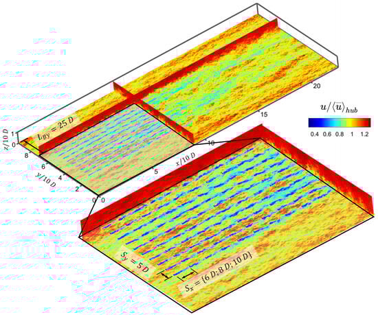
Figure 1.
Case setup with contour of simulated instantaneous wind speed in the wind farm.
4. Results
In this section, we present the LES results of wind turbine wakes in the simulated wind farms, focusing on the upward shift of wake centers. We employ and to denote the instantaneous and the corresponding time-averaged velocity, respectively, where the represents the time averaging. (same for the other two components) denotes the temporal velocity fluctuations, and denotes the Reynolds stress tensor. Velocity deficit is defined as , where is the time-averaged streamwise velocity at the inlet. is the spanwise average of at hub height, which is often employed as the characteristic velocity for normalization.
4.1. Phenomenon of Upward Shift of Wind Turbine Wakes on Wind Farms
Figure 2 first illustrates the upward shift of wind turbine wakes by examining mean velocity deficit contours at different downstream positions for case B. The wake center is defined as the position of maximum velocity deficit. Two approaches define the wake boundary: (1) the velocity deficit contour line with and (2) the intersection of a stream tube with the vertical plane, where the tube shape at matches the contour from approach 1. Upward shifts in the wake center are observed for the fifth and ninth turbine rows. Streamwise variations in the velocity deficit contour (white dashed line) show wake area expansion. To quantitatively demonstrate the upward shift of wind turbine wakes, Figure 3 shows the vertical profile of the wake velocity deficit in the middle plane behind the first, fifth, and ninth rows of wind turbines on the wind farm for Case B. As illustrated in the previous figure, the wake center of the first row of turbines consistently aligns with the hub height, regardless of the downwind turbine locations. Furthermore, the velocity profile exhibits a noticeable degree of symmetry around the wake center. These two characteristics serve as the foundation for the commonly used analytical wake models [8,9,10]. In contrast, for wind turbine wakes located deeper within the wind farm (e.g., the fifth and ninth rows as depicted in Figure 3), a noticeable upward shift of the wake center becomes apparent in the far wake region of the wind turbine. Additionally, the vertical velocity deficit profile ceases to exhibit symmetry around the wake center. The upward shift can be substantial, reaching approximately at a distance of downwind from the turbine, as depicted in Figure 3. Consequently, it becomes crucial to characterize these upward shifts, comprehend the underlying mechanisms, and effectively incorporate these effects into analytical wake models.
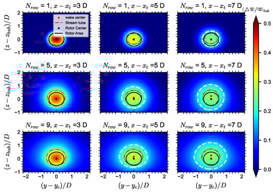
Figure 2.
Contours of mean streamwise velocity deficit averaged over turbines in the same row for the 1st, 5th and 9th rows for case B. The white dotted line represents the velocity deficit contour line (). The red dotted dashed line indicates the intersection of a stream tube, coinciding with the velocity contour at for each turbine, with the streamwise plane. The position of maximum velocity deficit is determined through quadratic spline interpolation of LES data, avoiding uncertainties in identifying the wake center.
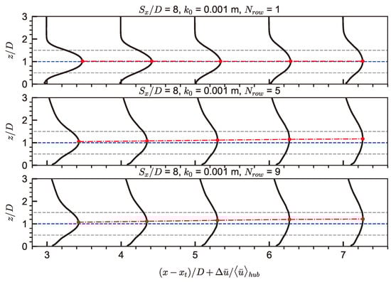
Figure 3.
Vertical distributions of the streamwise velocity deficit are shown at , , , , and downstream positions for the 1st, 5th, and 9th turbine rows in the wind farm with and m (black solid lines). The red dotted dashed line marks the wake center from the quadratic fitting function, avoiding data noise. The horizontal gray dotted lines represent the top and bottom turbine tips. The horizontal blue dotted line indicates the turbine hub height.
To delve deeper into the upward shift characteristics of wind turbine wakes, we examine the vertical profiles of the streamwise component of the Reynolds normal stresses and the primary Reynolds shear stress from Case B in Figure 4 and Figure 5, respectively.
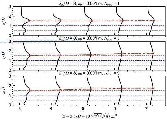
Figure 4.
Vertical distributions of the streamwise Reynolds normal stress are shown at , , , , and downstream for the 1st, 5th, and 9th turbine rows in the wind farm with and m (black solid lines). The red dotted dashed line marks the peak from the quadratic fitting, avoiding data noise. The horizontal gray dotted lines indicate the top and bottom turbine tips. The horizontal blue dotted line shows the turbine hub height.
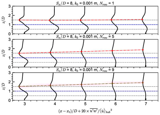
Figure 5.
Vertical distributions of the primary Reynolds shear stress are shown at , , , , and downstream for the 1st, 5th, and 9th turbine rows in the wind farm with and m (black solid lines). The red dotted dashed line marks the peak from the quadratic fitting, avoiding data noise. The horizontal gray dotted lines indicate the top and bottom turbine tips. The horizontal blue dotted line shows the turbine hub height.
In the case of the first row of wind turbines, it is evident that the vertical positions associated with the maximum magnitudes of and are in proximity to the top tip. Conversely, for the wakes of wind turbines in the fifth and ninth rows, these positions gradually shift upward in the downstream direction. When comparing Figure 4 and Figure 5 with Figure 3, it becomes evident that the extent of the upward shift in the Reynolds stresses mirrors that of the wake center.
We then examine the mean kinetic energy (MKE) budget to gain insights into the transfer of MKE within wind turbine wakes at various downstream turbine locations. The MKE budget equation employed for this analysis is as follows:
where MC, TC, and PT represent the MKE convection transport terms caused by mean convection, turbulent convection, and pressure, respectively, and TP represents the energy sink term from MKE to turbulent kinetic energy (TKE), and VD and D represent the MKE dissipation terms due to viscous and mean convection, respectively.
The terms of the MKE budget equation are illustrated in Figure 6, where averaging has been performed over turbines within the same row. As observed, the mean convective (MC) and turbulent convective (TC) terms dominate at the majority of turbine downwind positions. At a distance of 3D downstream from the turbine, the PT term, attributed to the energy extraction by this wind turbine, is nearly negligible. However, at a position 7D downstream from the turbine (1D upstream of the downwind turbine), the PT term becomes significant, owing to the blocking effect of the downwind turbine. It is evident in Figure 6 that turbulence entrainment plays a pivotal role in the wake recovery process for wind turbines located deep within a wind farm. An important observation is that the region exhibiting a high-magnitude TC term shifts upward as one progresses downwind, particularly for turbines in the fifth and ninth rows. Notably, the wake center almost aligns with the position where the TC term reaches its maximum magnitude.
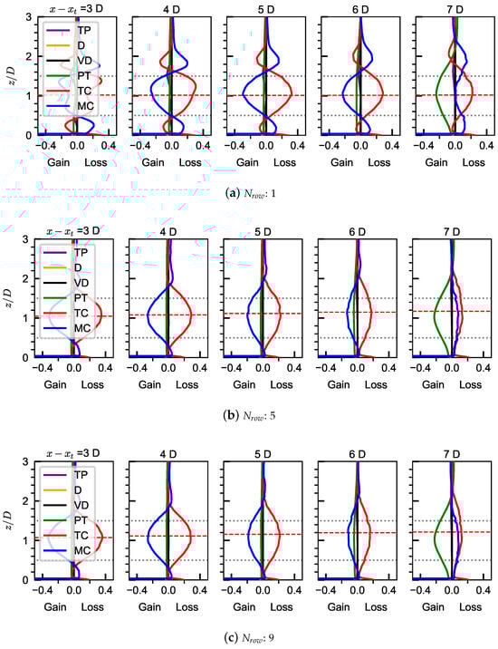
Figure 6.
Vertical distributions of the MKE budget terms in the middle plane (dimensionless by ) for the 1st, 5th and 9th rows of wind turbines for case B ( and m). The red dotted line indicates the location of the wake center, and the grey dotted lines represent the top and bottom tips of the rotor.
The upward shift of the wake center is mainly caused by two factors, i.e., the upward shift of the region with extensive turbulence convection (i.e., the TC term) and the ground-blocking effect. In the case of wind turbines in the first row, the majority of momentum entrainment happens within the wake and the influence of the ground is minimal because of the small wake width. However, for wind turbines situated deep within the farm, a significant amount of momentum entrainment happens above the top tip and the ground-blocking effect becomes significant because of the large wake width (as depicted in Figure 2), leading to a noticeable alteration in the vertical trajectory of the wake center.
In the following, we examine the effect of streamwise turbine spacing and ground roughness length on the upward shift of the wake center. Figure 7a illustrates the upward shift of wind wakes for wind farms with different streamwise turbine spacings (i.e., ). It is seen that the general trends of wake center from wind farms with different are highly consistent with each other. In contrast, for the cases with varying ground roughness lengths as depicted in Figure 7b, a more significant upward shift of the wake center is evident in cases with higher ground roughness lengths. This observation is in line with expectations since a larger wake width (because of a higher recovery rate) is associated with higher values of , leading to a more pronounced ground-blocking effect.
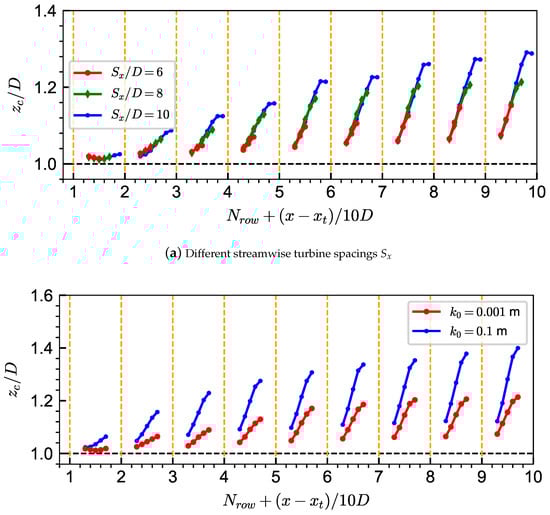
Figure 7.
The upward shift of wake centers for wind turbines in various rows is illustrated, with denoting the streamwise coordinate of each row’s turbine and representing the vertical coordinate of the wake center. To minimize the potential impact of data noise, a local fitting of the vertical velocity deficit profile is conducted before identifying the maximum value. The orange dotted line indicates the location of each row’s turbine.
4.2. Incorporation of the Upward Shift in Analytical Wake Models
In this section, we incorporate the upward shift of the wake center into the analytical wake models. The analytical model is developed using a methodology similar to the Jensen model [8], where mass conservation is enforced within a control volume starting from the near wake. Specifically in this work, the LES results give the velocity deficit at the inlet of the control volume, eliminating the necessity for a wake superposition model. We assume that the ambient flow velocity is uniform vertically, without considering the logarithmic law typical of atmospheric boundary layer flow.
To calculate the velocity in the wake of the i-th-row turbine () as shown in Figure 8, where x represents the streamwise distance relative to wind turbine , we apply mass conservation as follows:
where is the initial wake area at the inlet of the control volume (), and is the wake area at position x. In this work, the wake area is defined as the region a velocity deficit exceeding 5 % of . The above equation can be simplified to express the velocity deficit as follows:
where . Figure 9 illustrates that the wake shape may deviate from a perfect circle due to the influence of ground blocking and the changing wake recovery rate with distance from the ground. To simplify the problem, we divide the wake into upper and lower parts, each with its own recovery rate. With this simplification, the wake area can be calculated as follows:
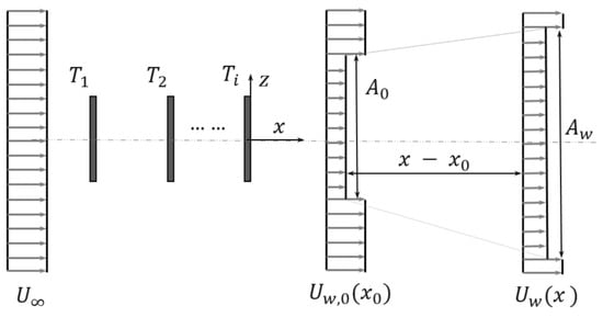
Figure 8.
Schematic of the analytical wake model with the gray dash-dotted line representing the wake center.
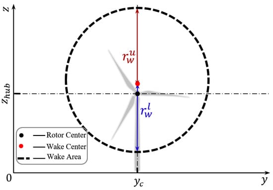
Figure 9.
Schematic of the wake area in the streamwise plane for case B. The black dotted line indicates a contour with a 5% velocity deficit . Red dots represent the wake center, and blue dots represent the rotor center.
For the lower part of the wake, we utilize the following linear expansion:
where and are the recovery rate and the initial wake radius, respectively. At more distant turbine downwind locations, may be less than the distance from the wake center to the ground (i.e., ). In such cases, . For the upper part of the wake, we use different expressions for various rows of wind turbines based on an analysis of the LES results. These expressions are as follows:
where and are the recovery rate and the initial wake radius, respectively, for the upper-part wake. In the present work, we directly specify the initial wake radius using the LES results. For the recovery rates, we first fit the upper and lower parts of the vertical velocity deficit profile separately using the Gaussian function and then compute and using the variances of the Gaussian fitted profiles ( and for the lower and upper parts of the wake, respectively) at different turbine downwind locations. Figure 10a illustrates the fitting of the vertical velocity deficit profile for both the upper and lower parts, along with the streamwise variations in the variances in the Gaussian fitted profiles.
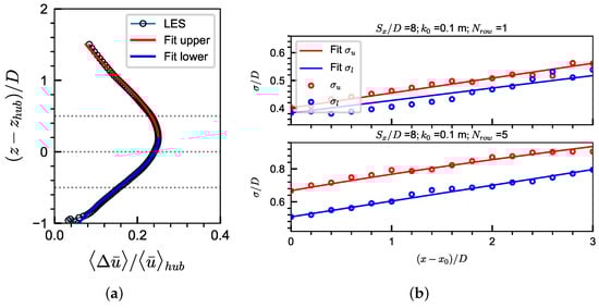
Figure 10.
Fitting of the vertical velocity deficit profiles using separate Gaussian functions for the lower and upper parts of the wake. (a) Gaussian-fitted and LES velocity deficit profiles at 5D downwind of the fifth-row turbine for case D ( and m). (b) Fitting of the streamwise variations of the variances ( and ) of the fitted Gaussian profiles.
Based on Equation (7), with given by the LES results and the wake area computed using Equation (8), the velocity deficit at any turbine downwind location can be computed. By employing two separate Gaussian profiles for the lower and upper parts of the wake, we determine the maximum velocity deficit () while adhering to the constraint of mass conservation as follows:
Thus far, we have computed the velocity deficit profiles at various turbine downwind locations, taking into account the ground effect and the distinct recovery rates for the lower and upper parts of the wake. In the following section, we will investigate the impact of the upward shift of the wake center. In one application of the analytical model derived above, we assume the wake center to be at the turbine’s hub height. In the other application, we use the wake center obtained from the LES results.
Figure 11 presents comparisons between the vertical velocity deficit profiles obtained from the analytical model and the corresponding LES results for Case D. The initial conditions for this case are detailed in Table 2. Both cases, with and without considering the upward shift of the wake center, show good agreement with the LES results for the wakes of the first and third rows of wind turbines. Discrepancies are observed at downwind for the wakes of the fifth, seventh, and ninth wind turbines, despite the mean velocity deficits being based on the LES results. These discrepancies primarily arise from the deviation of the upper part of the wake from the Gaussian function. At more distant turbine downwind locations, the model considering the upward shift of the wake center shows velocity deficits in good agreement with the LES results, whereas the model without the upward shift over-predicts the deficits.
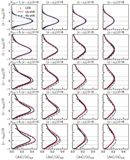
Figure 11.
Comparison of the velocity deficit profiles predicted by the analytical model with (red solid lines) and without (blue dashed lines) considering the upward shift of the wake center, with reference to the LES results for case D ( = 0.1 m). The gray dotted lines represent the top tip, bottom tip, and hub height positions.
Table 2.
Initial conditions of the analytical model for case D.
5. Conclusions
In this work, we investigated the vertical positions of wake centers for wind turbines within wind farms using large-eddy simulation with an actuator disk model. We considered four cases, including cases with three streamwise turbine spacings (i.e., ) with the ground roughness length 0.001 m, and a case with and 0.1 m.
The simulation results showed an upward shift of the wake center for wind turbines that sit deep within wind farms, such as those after three rows of wind turbines. It is observed that the wake center shifts upward at a higher rate for turbines in rows further downwind and for ground with larger roughness lengths. It is conjectured that such an upward shift of the wake center is due to the upward shift of the region with turbulence-dominated momentum entrainment, and the effect of the ground, which inhibits the expansion of the wake toward the ground.
An analytical wake model accounting for the upward shift of the wake center was proposed for computing the vertical distribution of velocity deficit. The model accounts for the ground effect and employs different recovery rates for the lower and upper parts of the wake. Comparison with the LES results showed a better agreement for the analytical wake model considering the upward shift of the wake center. It is noted that the initial velocity deficit at the near wake location (i.e., turbine downwind in this work) as well as the wake recovery rate and the upward shift are given by the LES results in the employed analytical wake model. Further development is required to account for the wake superposition in wind farms and to model the interaction of the wake with the atmospheric boundary layer.
The Coriolis force has not been taken into account in the simulations. The atmospheric stability condition is assumed to be neutral. These are the two significant factors that have not been considered in this study, and it is important to keep them in mind when interpreting the presented results. Other factors, such as the employed wind turbine parameterization model, turbulence model, and discretization scheme may introduce uncertainties to the simulation results. Uncertainty analysis on how they affect the simulation results is important especially for the development of computational methods. However, it is beyond the scope of this work and should be investigated in future work.
Author Contributions
Conceptualization, X.Y. and Z.W.; methodology, X.Y. and Z.W.; software, X.Y.; validation, Z.W.; formal analysis, Z.W.; investigation, Z.W. and X.Y.; writing—original draft preparation, Z.W.; writing—review and editing, X.Y.; visualization, Z.W.; supervision, X.Y.; project administration, X.Y.; funding acquisition, X.Y. All authors have read and agreed to the published version of the manuscript.
Funding
This work was supported by the NSFC Basic Science Center Program for “Multiscale Problems in Nonlinear Mechanics” (No. 11988102), the National Natural Science Foundation of China (No. 12172360), the Institute of Mechanics CAS, and the Chinese Academy of Sciences.
Data Availability Statement
The data presented in this study are available on request from the corresponding author.
Conflicts of Interest
The authors declare no conflict of interest.
References
- Stevens, R.J.; Meneveau, C. Flow structure and turbulence in wind farms. Annu. Rev. Fluid Mech. 2017, 49, 311–339. [Google Scholar] [CrossRef]
- Porté-Agel, F.; Bastankhah, M.; Shamsoddin, S. Wind-turbine and wind-farm flows: A review. Bound.-Layer Meteorol. 2020, 174, 1–59. [Google Scholar] [CrossRef] [PubMed]
- Chamorro, L.P.; Porté-Agel, F. A wind-tunnel investigation of wind-turbine wakes: Boundary-layer turbulence effects. Bound.-Layer Meteorol. 2009, 132, 129–149. [Google Scholar] [CrossRef]
- Wu, Y.T.; Porte-Agel, F. Atmospheric turbulence effects on wind-turbine wakes: An LES study. Energies 2012, 5, 5340–5362. [Google Scholar] [CrossRef]
- Xie, S.; Archer, C. Self-similarity and turbulence characteristics of wind turbine wakes via large-eddy simulation. Wind Energy 2015, 18, 1815–1838. [Google Scholar] [CrossRef]
- Yang, X.; Sotiropoulos, F.; Conzemius, R.J.; Wachtler, J.N.; Strong, M.B. Large-eddy simulation of turbulent flow past wind turbines/farms: The Virtual Wind Simulator (VWiS). Wind Energy 2015, 18, 2025–2045. [Google Scholar] [CrossRef]
- Göçmen, T.; Van der Laan, P.; Réthoré, P.E.; Diaz, A.P.; Larsen, G.C.; Ott, S. Wind turbine wake models developed at the technical university of Denmark: A review. Renew. Sustain. Energy Rev. 2016, 60, 752–769. [Google Scholar] [CrossRef]
- Jensen, N. A note on wind turbine interaction. In Riso-M-2411; Risoe National Laboratory: Roskilde, Denmark, 1983; p. 16. [Google Scholar]
- Frandsen, S.; Barthelmie, R.; Pryor, S.; Rathmann, O.; Larsen, S.; Højstrup, J.; Thøgersen, M. Analytical modelling of wind speed deficit in large offshore wind farms. Wind Energy 2006, 9, 39–53. [Google Scholar] [CrossRef]
- Bastankhah, M.; Porté-Agel, F. A new analytical model for wind-turbine wakes. Renew. Energy 2014, 70, 116–123. [Google Scholar] [CrossRef]
- Ge, M.; Wu, Y.; Liu, Y.; Yang, X.I. A two-dimensional Jensen model with a Gaussian-shaped velocity deficit. Renew. Energy 2019, 141, 46–56. [Google Scholar] [CrossRef]
- Lissaman, P. Energy effectiveness of arbitrary arrays of wind turbines. J. Energy 1979, 3, 323–328. [Google Scholar] [CrossRef]
- Gao, X.; Li, B.; Wang, T.; Sun, H.; Yang, H.; Li, Y.; Wang, Y.; Zhao, F. Investigation and validation of 3D wake model for horizontal-axis wind turbines based on filed measurements. Appl. Energy 2020, 260, 114272. [Google Scholar] [CrossRef]
- Ling, Z.; Zhao, Z.; Liu, Y.; Liu, H.; Liu, Y.; Ma, Y.; Wang, T.; Wang, D. A three-dimensional wake model for wind turbines based on a polynomial distribution of wake velocity. Ocean Eng. 2023, 282, 115064. [Google Scholar] [CrossRef]
- Zhang, S.; Gao, X.; Ma, W.; Lu, H.; Lv, T.; Xu, S.; Zhu, X.; Sun, H.; Wang, Y. Derivation and verification of three-dimensional wake model of multiple wind turbines based on super-Gaussian function. Renew. Energy 2023, 215, 118968. [Google Scholar] [CrossRef]
- Crespo, A.; Hernández, J.; Frandsen, S. Survey of modelling methods for wind turbine wakes and wind farms. Wind Energy 1999, 2, 1–24. [Google Scholar] [CrossRef]
- Gunn, K.; Stock-Williams, C.; Burke, M.; Willden, R.; Vogel, C.; Hunter, W.; Stallard, T.; Robinson, N.; Schmidt, S. Limitations to the validity of single wake superposition in wind farm yield assessment. J. Phys. Conf. Ser. 2016, 749, 012003. [Google Scholar] [CrossRef]
- Zong, H.; Porté-Agel, F. A momentum-conserving wake superposition method for wind farm power prediction. J. Fluid Mech. 2020, 889, A8. [Google Scholar] [CrossRef]
- Bastankhah, M.; Welch, B.L.; Martínez-Tossas, L.A.; King, J.; Fleming, P. Analytical solution for the cumulative wake of wind turbines in wind farms. J. Fluid Mech. 2021, 911, A53. [Google Scholar] [CrossRef]
- Niayifar, A.; Porté-Agel, F. Analytical modeling of wind farms: A new approach for power prediction. Energies 2016, 9, 741. [Google Scholar] [CrossRef]
- Katic, I.; Højstrup, J.; Jensen, N.O. A simple model for cluster efficiency. In Proceedings of the European Wind Energy Association Conference and Exhibition—A Raguzzi, Rome, Italy, 7–9 October 1986; Volume 1, pp. 407–410. [Google Scholar]
- Sun, H.; Yang, H. Numerical investigation of the average wind speed of a single wind turbine and development of a novel three-dimensional multiple wind turbine wake model. Renew. Energy 2020, 147, 192–203. [Google Scholar] [CrossRef]
- Liu, X.; Li, Z.; Yang, X.; Xu, D.; Kang, S.; Khosronejad, A. Large-eddy simulation of wakes of waked wind turbines. Energies 2022, 15, 2899. [Google Scholar] [CrossRef]
- Chamorro, L.P.; Porte-Agel, F. Turbulent flow inside and above a wind farm: A wind-tunnel study. Energies 2011, 4, 1916–1936. [Google Scholar] [CrossRef]
- Zhang, F.; Yang, X.; He, G. Multiscale analysis of a very long wind turbine wake in an atmospheric boundary layer. Phys. Rev. Fluids 2023, 8, 104605. [Google Scholar] [CrossRef]
- Johlas, H.M.; Schmidt, D.P.; Lackner, M.A. Large eddy simulations of curled wakes from tilted wind turbines. Renew. Energy 2022, 188, 349–360. [Google Scholar] [CrossRef]
- Yang, X.; Angelidis, D.; Khosronejad, A.; Le, T.; Kang, S.; Gilmanov, A.; Ge, L.; Borazjani, I.; Calderer, A. Virtual Flow Simulator. [Computer Software]. 2015. Available online: https://www.osti.gov/doecode/biblio/4195 (accessed on 7 December 2023). [CrossRef]
- Calderer, A.; Yang, X.; Angelidis, D.; Khosronejad, A.; Le, T.; Kang, S.; Gilmanov, A.; Ge, L.; Borazjani, I. Virtual Flow Simulator; Technical report; Univ. of Minnesota: Minneapolis, MN, USA, 2015. [Google Scholar]
- Yang, X.; Sotiropoulos, F. On the predictive capabilities of LES-actuator disk model in simulating turbulence past wind turbines and farms. In Proceedings of the 2013 American Control Conference, Washington, DC, USA, 17–19 June 2013; IEEE: Manhattan, NY, USA, 2013; pp. 2878–2883. [Google Scholar]
- Germano, M.; Piomelli, U.; Moin, P.; Cabot, W.H. A dynamic subgrid-scale eddy viscosity model. Phys. Fluids A Fluid Dyn. 1991, 3, 1760–1765. [Google Scholar] [CrossRef]
- Li, Z.; Liu, X.; Yang, X. Review of turbine parameterization models for large-eddy simulation of wind turbine wakes. Energies 2022, 15, 6533. [Google Scholar] [CrossRef]
- Dong, G.; Li, Z.; Qin, J.; Yang, X. Predictive capability of actuator disk models for wakes of different wind turbine designs. Renew. Energy 2022, 188, 269–281. [Google Scholar] [CrossRef]
- Yang, X.; Zhang, X.; Li, Z.; He, G.W. A smoothing technique for discrete delta functions with application to immersed boundary method in moving boundary simulations. J. Comput. Phys. 2009, 228, 7821–7836. [Google Scholar] [CrossRef]
- Yang, X.; Kang, S.; Sotiropoulos, F. Computational study and modeling of turbine spacing effects in infinite aligned wind farms. Phys. Fluids 2012, 24, 115107. [Google Scholar] [CrossRef]
- Ge, L.; Sotiropoulos, F. A numerical method for solving the 3D unsteady incompressible Navier–Stokes equations in curvilinear domains with complex immersed boundaries. J. Comput. Phys. 2007, 225, 1782–1809. [Google Scholar] [CrossRef]
- Wang, Z.; Dong, G.; Li, Z.; Yang, X. Statistics of wind farm wakes for different layouts and ground roughness. Bound.-Layer Meteorol. 2023, 188, 285–320. [Google Scholar] [CrossRef]
Disclaimer/Publisher’s Note: The statements, opinions and data contained in all publications are solely those of the individual author(s) and contributor(s) and not of MDPI and/or the editor(s). MDPI and/or the editor(s) disclaim responsibility for any injury to people or property resulting from any ideas, methods, instructions or products referred to in the content. |
© 2023 by the authors. Licensee MDPI, Basel, Switzerland. This article is an open access article distributed under the terms and conditions of the Creative Commons Attribution (CC BY) license (https://creativecommons.org/licenses/by/4.0/).