1. Introduction
Global warming and environmental pollution are among the most important problems of our age due to high carbon emissions. Numerous types of human activity are associated with
emissions [
1,
2]. Transport, namely land transportation, is one of these categories [
3]. Nowadays, 99.8% of the worldwide transportation system relies on internal combustion engines (ICEs), and approximately 95% of the energy used in transportation is derived from liquid fuels derived from petroleum sources [
4]. In the European transportation sector, the highest portion of emissions, amounting to 60.7%, is attributed to passenger cars [
5]. Nearly 72% of all
emissions in the European Union are produced by the transportation industry [
6]. Therefore, countries have started to find new solutions for reducing carbon emissions [
7,
8]. The idea has come to the force to develop methods enabling vehicles that consume less energy to travel long distances and use internal combustion engines less. Therefore, hybrid vehicles have been developed that will enable both electric motors and ICE to operate simultaneously. The European Automotive Market has turned towards electric vehicles since the effects of climate change became more prominent on the continent. However, there has also been a significant increase in the registration of fully hybrid vehicles, which offsets the increased carbon dioxide emissions from electric vehicles [
9].
Various techniques have been established in the literature to guarantee the control and fuel efficiency of hybrid vehicles. One of the most commonly used fuel efficiency methods is rule-based control because it is easy to apply. According to the power required during the driving cycle, rule-based control approaches have been developed in the literature. Hybrid electric vehicles (HEVs) are complex systems comprising internal combustion engines, electric motors, batteries, and a range of energy storage and conversion elements [
10,
11,
12]. Shabbir et al. proposed that rule-based control strategies effectively optimize the energy management of hybrid electric vehicles, and the modification of thresholds in the rules contributes to the sustainability of hybrid vehicle charging and fuel utilization [
10]. Ding et al. suggested a hybrid energy management system for the series-parallel plug-in hybrid electric vehicle (PHEV) by employing a rule-based control strategy and an optimization technique based on genetic algorithms (GA) to address the constraints of the battery [
11]. An almost optimal rule-based mode control (RBC) strategy was proposed for a specific plug-in hybrid electric vehicle (PHEV), considering the losses in the drivetrain, by Son et al. [
12]. Loss models were created for individual drivetrain components such as gears, planetary gears (PG), bearings, and the oil pump using both experimental data and mathematical governing equations [
12]. Li et al. proposed an innovative rule-based control strategy for parallel hybrid electric vehicles (HEVs), named the Torque-Leveling Threshold-Changing Strategy (TTS) [
13]. The TTS incorporates a recently introduced torque-leveling approach along with an improved threshold-changing mechanism derived from its previous implementations in series hybrid electric vehicles (HEVs) [
13]. Padmarajan developed the blended rule-based energy management system (EMS) for a plug-in hybrid electric vehicle [
14]. During the assessment, the parallel plug-in hybrid electric vehicle (PHEV) architecture underwent simulations for various real-world destinations with unpredictable trip demands, mimicking real-world driving conditions. The suggested energy management system (EMS) demonstrated a fuel economy enhancement of up to 18.4%, accompanied by a reduction of engine stop-start occurrences by a factor of nine when compared to the traditional rule-based EMS [
14]. Peng et al. proposed a rule-based energy management strategy for a plug-in hybrid school bus [
15]. The rule-based energy management strategy consumed 13.7 L of fuel per 100 km with a 75% critical state of charge [
15]. In addition, Peng et al. utilized dynamic programming to adjust and optimize a rule-based energy management strategy [
16]. Therefore, the fuel consumption was reduced by 10.45% with the proposed method [
16]. Zhu discussed the assessment of energy consumption weighted by the utility factor employing a rule-based strategy in the context of a real-world representative drive cycle [
17].
Another control method for fuel consumption is the equivalent consumption minimization strategy (ECMS) based on the equivalent fuel consumption of the battery energy [
18,
19]. Paganelli et al. achieved a fuel saving of 17.5% by using the ECMS method for the European Normalized Cycle [
18]. Zhang investigated the impact of incorporating terrain, vehicle speed, and trip distance preview on improving the fuel efficiency of plug-in hybrid vehicles. The availability of future information is categorized into full, partial, or no future information, and a corresponding energy management strategy with potential real-time implementation is proposed for each case. Dynamic Programming (DP) served as a benchmark for scenarios with complete knowledge of future driving conditions. The Equivalent Consumption Minimization Strategy (ECMS) was employed as an instantaneous real-time minimization strategy, with parameters adjusted based on estimated future driving conditions obtained from DP or a backward solution of ECMS [
19].
Additionally, the fuzzy logic control system used in hybrid vehicles also makes it simple to study the complex structure of the vehicle because it is built from fuzzy sets. To adapt the powertrains and offer the best fuel efficiency, the fuzzy logic control system is used by Arıkuşu et al., Ma et al., and Sher et al. [
20,
21,
22]. Arıkuşu et al. designed a fuzzy logic controller for a hybrid electric vehicle, intended to assess the engine’s operational conditions within the hybrid control unit by utilizing sensor data [
20]. Ma investigated the energy management of a parallel hybrid electric vehicle (HEV), focusing on the fuel economy and battery state of charge (SOC) under NEDC and WLTC driving cycles with the fuzzy logic control strategy [
21]. The numerical analysis showed that implementing the fuzzy logic control strategy resulted in a 13.3% decrease in fuel consumption during the NEDC driving cycle and a 4.5% decrease during the WLTC driving cycle compared to the logic threshold control strategy [
21]. Sher et al. suggested that the fuzzy logic algorithm can reduce fuel consumption by 5%, reduce CO emissions by 50%, and increase the operational efficiency of the engine by 15% [
22]. The internal combustion engine, electric motor, transmission, and battery efficiency of the vehicle were ideally adjusted utilizing the fuzzy logic method for fuel consumption by Suhail et al. and Saju et al. [
23,
24]. Moreover, a hybrid vehicle’s energy-efficient system uses an adaptive neuro-fuzzy inference system (ANFIS) developed by Suhail et al. and Saju et al. [
23,
24]. ANFIS improved the performance and fuel efficiency of hybrid electric vehicles. ANFIS and fuzzy control-based energy management systems have shown promising results in the theoretical and simulation phases, but their real-time implementation has proven to be challenging.
On the other hand, metaheuristic algorithms have also been used to increase energy efficiency for hybrid vehicles [
25,
26,
27,
28,
29,
30]. Chen presented an energy management strategy incorporating a particle swarm optimization (PSO) algorithm. Energy consumption experienced reductions of 1.99% and 3.72% for the two driving cycles conducted within the loop experiment [
25]. Wang et al. examined the parameters of hybrid vehicle transmission systems, considering the objective function, decision variables, and constraints [
26]. The NSGA-II algorithm was utilized, resulting in a 13.25% decrease in energy consumption and an improvement in efficiency [
26]. Hegazy et al. proposed the particle swarm optimization (PSO) technique to minimize hydrogen consumption and minimize the cost, mass, and volume of the energy storage system for fuel cell hybrid electric vehicles according to the driving cycle [
27]. In addition, the butterfly optimization algorithm was used for energy management by Prasanthi et al. [
28]. A master-slave hybrid electric vehicle (MSHEV) with multiple energy sources was presented by Zhang et al. [
29]. The optimization objective chosen was the battery state of charge for MSHEV, and relevant parameters were optimized. Subsequently, an approximate model was developed using the Response Surface Model, and an optimization model was created utilizing the Multi-Island Genetic Algorithm. He et al. conducted an optimization study on engine control parameters, implementing it on a PHEV with a rule-based energy management strategy (EMS) to enhance the fuel efficiency of a PHEV engine [
30]. They introduced a control parameter optimization approach based on the engine’s equivalent operating point, proposing the optimization of four crucial engine control parameters using a genetic algorithm (GA). In the literature, metaheuristic algorithm results have been shown to maximize energy efficiency and minimize fuel consumption. Nevertheless, metaheuristic algorithms still pose challenges when applied to real-time systems due to their stochastic solutions.
Machine learning is the field of enabling computers to perform tasks without explicit programming, with applications ranging from the development of intelligent robots (for tasks like perception and control) to text comprehension, computer vision, medical informatics, audio analysis, database mining, and various other domains [
31]. In the literature, there are some studies on driving cycle prediction and energy consumption prediction for hybrid electric vehicles. He et al. proposed an approach for forecasting driving cycles by leveraging real-time traffic data obtained through vehicle-to-infrastructure (V2I) communication. They employed neural networks to make velocity predictions based on this data [
32]. Artificial Neural Networks (ANNs), functioning as machine learning algorithms, find applications in a variety of tasks, including classification, prediction, pattern recognition, and clustering. Sun et al. presented three prediction techniques, such as exponentially varying, the Markov process, and Artificial Neural Networks (ANNs) [
33]. These prediction methods are applied within each receding horizon, and the resulting velocity predictions are employed for optimizing energy consumption in a power-split Hybrid Electric Vehicle (HEV). The findings demonstrate that the ANN-based velocity predictor delivers the most effective performance in terms of predictive energy management. Hua et al. proposed an estimation model for electric vehicle energy consumption based on both vehicle parameters, such as speed and environmental data (e.g., GPS position and temperature), with a machine learning algorithm [
34]. In addition, ML has been widely used to control the fuel economy of hybrid electric vehicles [
35,
36,
37,
38]. Harold et al. developed a framework that would allow supervised machine learning to automatically retrain the supervisory powertrain control approach for hybrid electric vehicles [
35]. This framework consists of a combination of dynamic programming and supervised machine learning based on fuel consumption. Son et al. proposed an advanced rule-based control strategy with ML taking into account the driving cycle characteristics and present battery state of charge (SOC) for plug-in hybrid electric vehicles [
36]. Madziel et al. suggest a method for developing
emission models that require little computational effort and produce workable outcomes for fully hybrid vehicles [
37]. The Gaussian process regression method provided the best fit for the road input data used to create the
emission model. Kwon investigated a control map generation technique based on ML and optimization data for a multimode hybrid electric car [
38].
In this article, a control algorithm has been developed to reduce carbon emissions by estimating fuel consumption and using energy resources more efficiently. The aim of this study is to reduce carbon emissions by predicting fuel consumption and using energy resources more efficiently.
The contributions of this study are summarized as follows:
In this study, the modeling and verification of the electric motor, battery, and internal combustion engine of the hybrid electric vehicle produced within the scope of our TÜBİTAK ARDEB 1003 project titled “Development of Fuel Efficiency Enhancing and Innovative Technologies for Internal Combustion Engine Vehicles” were carried out. A new dataset was produced by an experiment model in the driving cycles for fuel consumption prediction of a parallel hybrid electric vehicle with a rule-based control algorithm.
In the literature, only road information is taken as an input value for estimation. The dataset created for this study contains 11 inputs (EM speed, EM torque, EM power, ICE speed, ICE torque, ICE power, driving cycle speed, driving cycle acceleration, fuel mass, forces, and SOC) and 1 output (fuel consumption). Thus, it is planned to obtain better results for fuel estimation by creating a more complex data set.
Using normalized training data, training was conducted for seven different machine learning methods. Then, tests were performed for each method using the normalized test data. For the purpose of normalization, the algorithms were kept from overfitting the data set. The normalized test data were created by hiding the amount of fuel to be estimated in the data set. Here, each method tries to produce the most appropriate predictive value by using the weight coefficients obtained as a result of the training and by looking at the fuel consumption values whose regression is desired in the test. Due to the large data set, the usual ratio of test data were chosen as 25% and 1.7%. Afterwards, predictions were made with both test data.
Fuel estimation was made with machine learning methods for 1.7% test data. The random forest algorithm 97.16%, REP tree 94.2%, M5P algorithm 93.54%, random tree algorithm 91.58%, multilayer perceptron algorithm 16%, linear regression 81.3%, and decision stump 80.36% have successfully estimated fuel consumption.
Fuel estimation was made with machine learning methods for 25% of the test data. The random forest algorithm 90.21%, random tree algorithm 86.68%, REP tree 84.18%, M5P algorithm 23.06%, multilayer perceptron algorithm 64.81%, linear regression 0.1%, and decision stump 23.74% have successfully estimated fuel consumption.
Based on the results, the vehicle powered by the proposed method uses 4.72 L of fuel per 100 km, compared to the gasoline-powered vehicle’s 7 L per 100 km. Additionally, the proposed method results in a reduction of 4.69 kg of emissions.
The Random Forest algorithm has been the most appropriate method in terms of training and test fuel consumption models, with , MAE and RMSE simulations suitable for both test datasets. The Random Forest Algorithm’s effectiveness has been validated through both simulated results and real-time data.
This paper is structured as follows: The mathematical model of the hybrid electric vehicle, control method, and data set are described in
Section 2. In
Section 3, machine learning algorithms and performance calculations are described. The simulation results and discussion for fuel consumption prediction are given in
Section 4. Some concluding remarks and future studies are described in
Section 5.
2. Models and Methodology
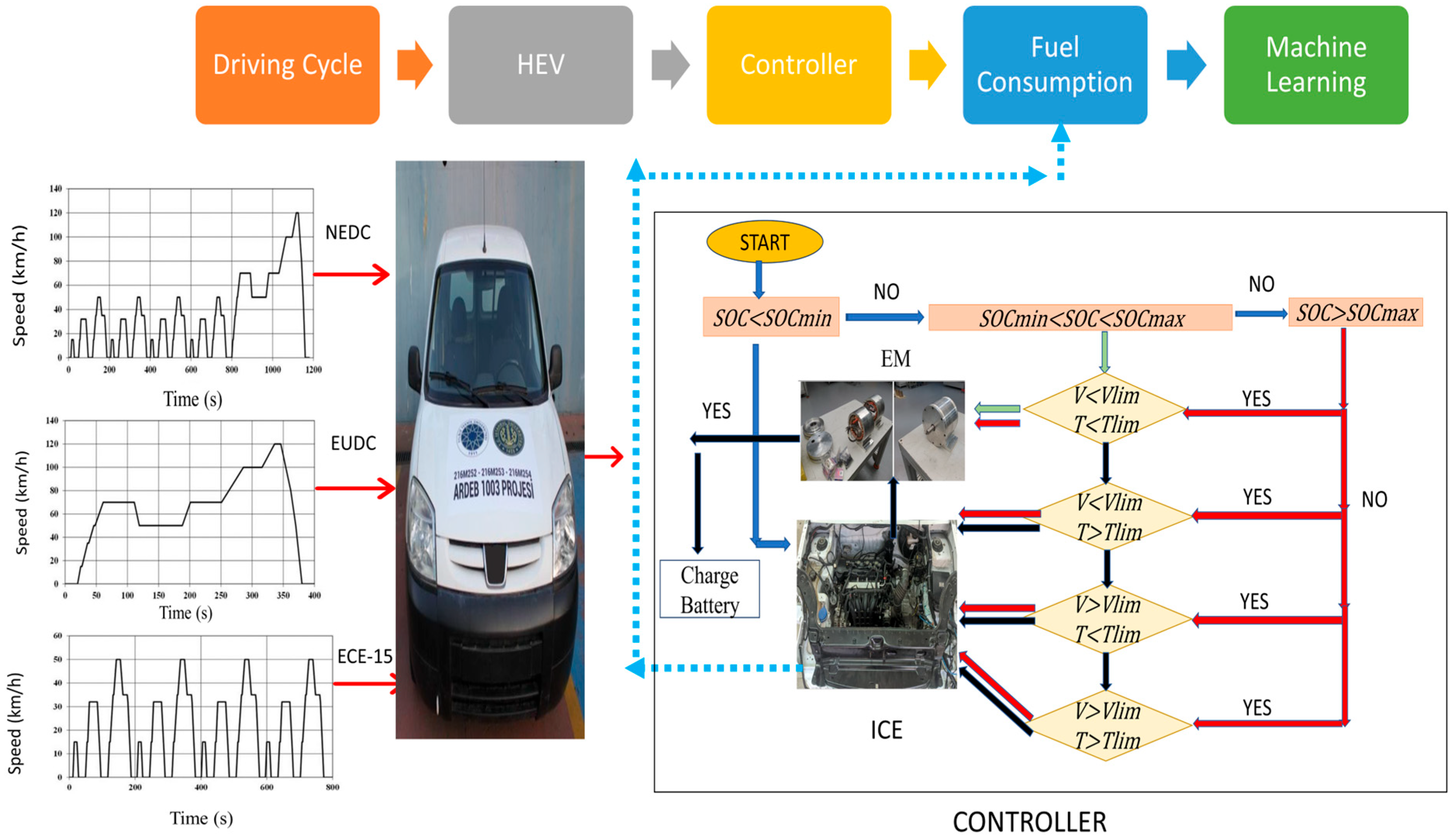
In this study, fuel consumption was evaluated using a machine learning method for the hybrid electric vehicle. It developed a dataset of real-time driving cycles and corresponding fuel consumption data. The dataset generation phase of the parallel hybrid electric vehicle is shown in
Figure 1. A driving cycle, a vehicle model, an electric motor model, and an internal combustion engine model are employed in
Figure 1. In this study, the speed values in the driving cycles were applied to the vehicle on a closed track, and the instantaneous fuel consumption values were recorded. The values were then transferred to MATLAB to calculate the speed and power values of the electric motor, the specific fuel consumption values of the internal combustion engine, and the power values of the internal combustion engine. During the calculation, firstly, the velocity and acceleration values of the vehicle were taken, and the forces acting on the vehicle were obtained. The mathematical model is as follows:
where
: traction force,
: rolling resistance,
: hill resistance,
: air resistance,
: density of air,
A: the cross-sectional area of the vehicle,
V: velocity,
: aerodynamic coefficient,
m: vehicle mass,
g: gravity acceleration,
: slope,
acceleration is expressed. Then, the power of the electric motor, the power of the internal combustion engine, the battery, and the transmission are created by the MATLAB QSS Toolbox [
39].
The energy consumption control component depicted in
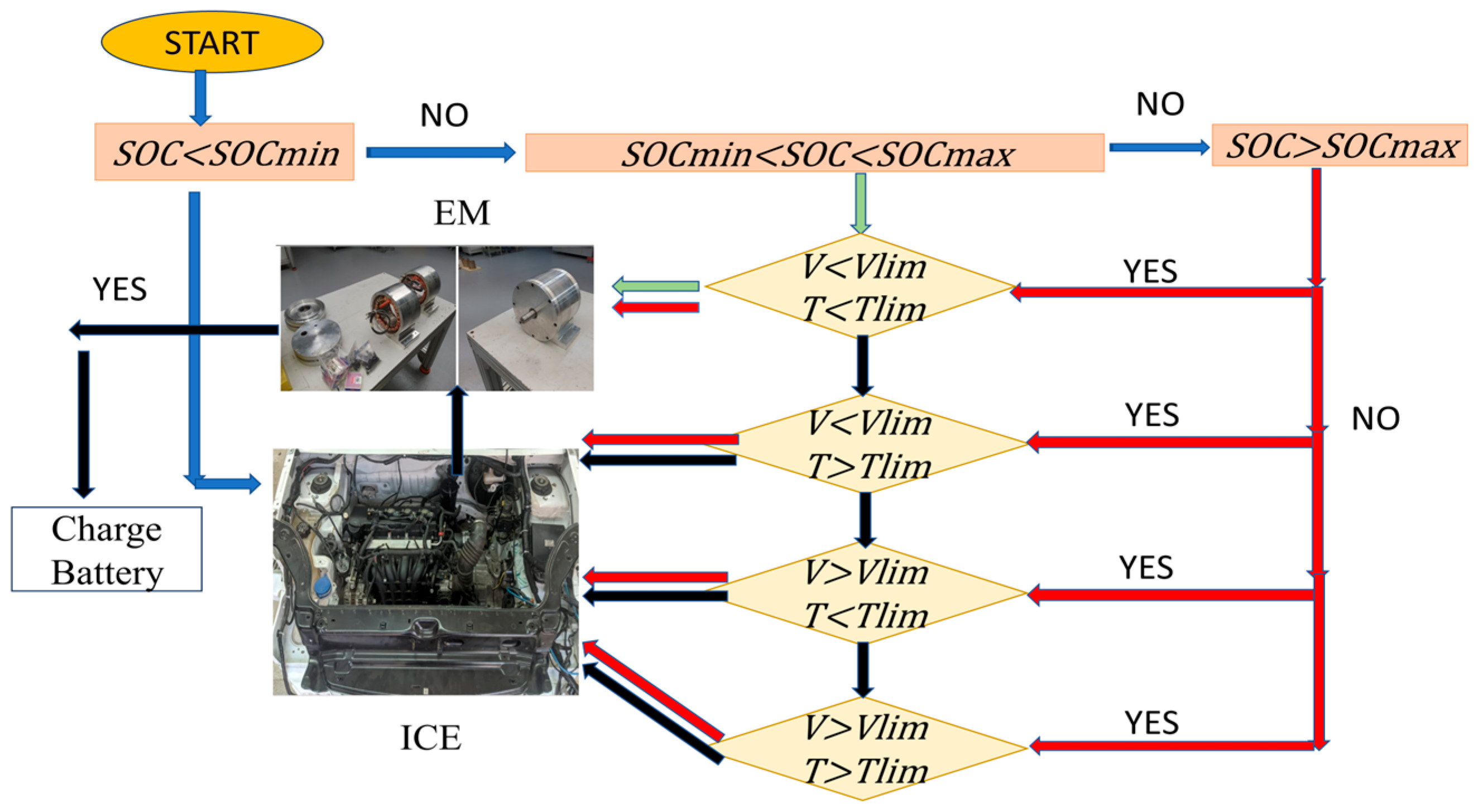
Figure 1 was created with consideration for the disparity between the power needed by the driver at any given time and the power generated by the internal combustion engine. The internal combustion engine is utilized when there is a requirement for higher power output. An electric motor is utilized as the main source of power when the power need is less than the capacity of the internal combustion engine. In addition to the power required for the electric motor to operate, SOC is also considered. An energy regulation system has been developed, adhering to the prescribed minimum and maximum SOC constraints. The vehicle’s design ensures operation with an electric motor until it attains a velocity of 40 km/h. After reaching a velocity exceeding 40 km/h, the internal combustion engine will be engaged. The internal combustion engine will function in areas characterized by low carbon emissions with respect to specific fuel consumption. Furthermore, as the speed decreases, the motor’s kinetic energy is converted into electrical energy, which is then directed towards recharging the battery. For this reason, an algorithm for a flow chart for the HEV Energy controller has been developed and shown in
Figure 2.
In
Figure 2,
V: speed,
: Electric motor maximum speed (40 km/h),
T: gearbox torque value and
: Electric motor maximum torque value (80 Nm).
: minimum value of SOC (% 45),
: maximum value of SOC (% 70) are expressed. The vehicle parameters are given in
Table 1 [
24].
When SOC value is range
, the speed and torque values receive low values, and EM works. The green arrows in
Figure 2 show that EM is working, and the black arrows show that ICE is working. Moreover, the battery value is not at its maximum level, and the excess energy obtained from ICE is transferred to EM, and EM works as a generator. Thus, the battery charges. When
Figure 2 is examined, in order for the vehicle to move with the electric motor, speed and torque values must be low, and SOC is the range at
or
. ICE works in all circumstances other than these constraints. In addition, the excess torque generated by the internal combustion engine is transferred to the electric motor, enabling the electric motor to work as a generator. Therefore, energy savings are achieved. The simulation study on the energy control strategy of a parallel hybrid vehicle is conducted using the vehicle parameters outlined in
Figure 1,
Figure 2, and
Table 1.
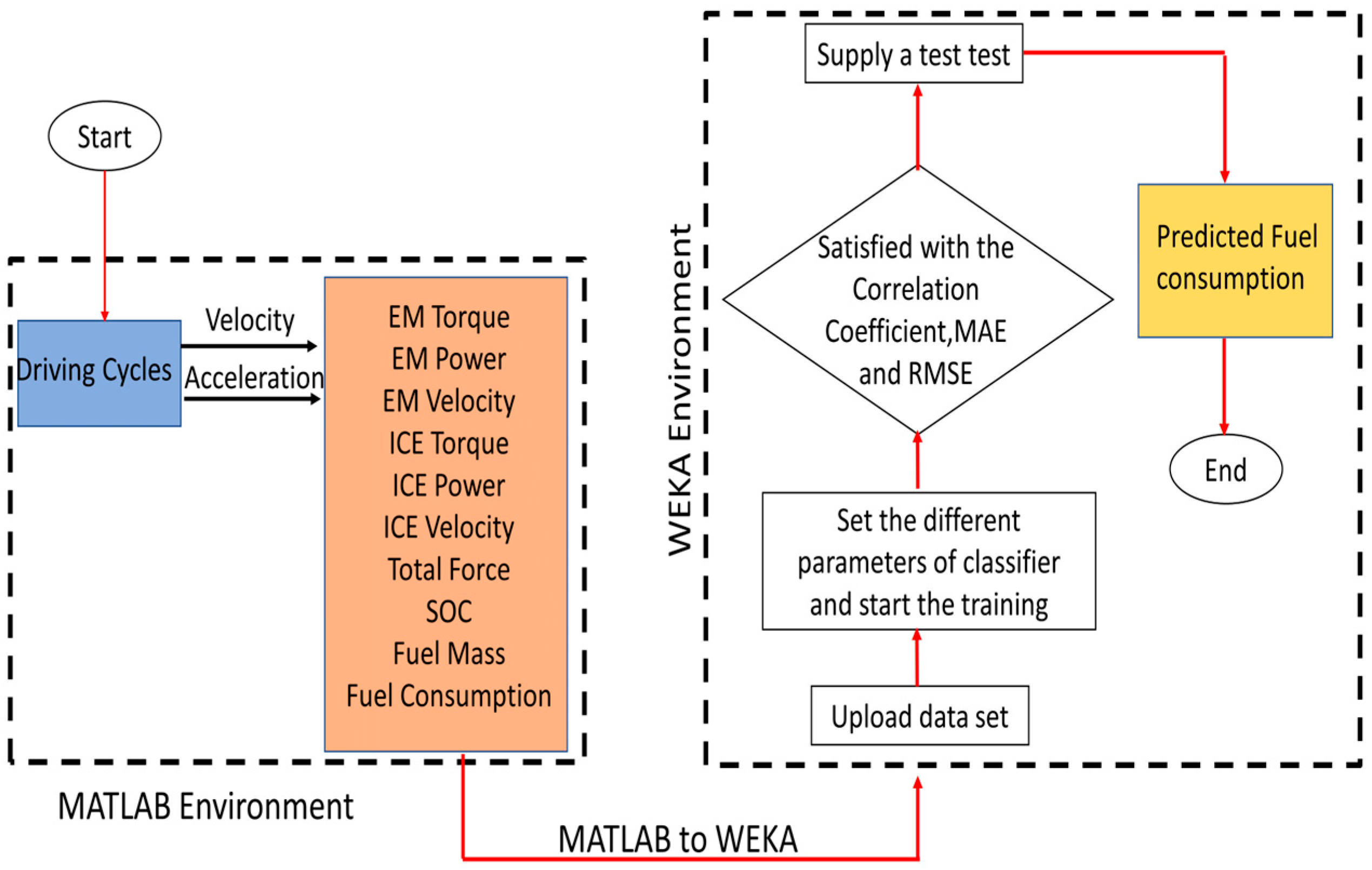
A novel dataset was generated to estimate fuel consumption for a parallel hybrid electric vehicle. This dataset was obtained by applying the ECE-15, EUDC, and NEDC driving cycles under controlled conditions on a traffic-free racetrack while employing the suggested control method. Afterwards, the speed, power, and torque information of the electric motor and the internal combustion engine were recorded for the data set in line with the information from the driving cycles in MATLAB. The flowchart of the data set are given in
Figure 3.
The dataset includes the angular speed values of the electric motor, the power values of the electric motor, the torque values of the electric motor, the angular speed values of the internal combustion engine, the torque values of the internal combustion engine, the power values of the internal combustion engine, the force values affecting the vehicle, the speed and driving cycle acceleration values, the fuel mass values, and the average fuel consumption of the vehicle. The whole dataset consists of 37,703 data points. Initially, a training-test separation rate of 1.7% was chosen for the machine learning model. Of the total dataset, 37,048 are used for training, and 655 are reserved for testing. In the testing phase, 1.7% of the total data were used to evaluate the fuel consumption prediction. Then, 28,876 of the datasets were used for training, and 9427 samples were reserved for testing. In the testing phase, 25% of the total data were used to evaluate the fuel consumption prediction. To avoid the risk of overfitting, the training-test decomposition ratio was chosen at 25% and 1.7%. This is to prevent the algorithms from overfitting the dataset. Fuel consumption values in the test data were hidden and created in this study.
The min-max normalization method is used to linearly normalize the data. The purpose of normalization is to ensure a comparison between the data. The minimum value can be at least equal to 0, while the maximum value can be equal to 1. Other values can be between 0 and 1. In the normalization method, values can only be between 0 and 1. The min-max normalization Method is given as
where
a,
,
,
denote normalized value, value to normalize, minimum value and maximum value, respectively. Normalized test and training data were used to predict fuel consumption using machine learning methods.
4. Results and Discussion
The experimental data were imported into MATLAB to compute the vehicle’s State of Charge (SOC), the overall power of the driving cycle, as well as the speed and power profiles of both the electric motor and internal combustion engine. Then, fuel consumption estimation was performed for the data set obtained from the experiment.
The outcomes derived from the machine learning algorithm, as applied in conjunction with the suggested control approach, are presented in
Figure 5,
Figure 6,
Figure 7,
Figure 8 and
Figure 9 for the NEDC cycle.
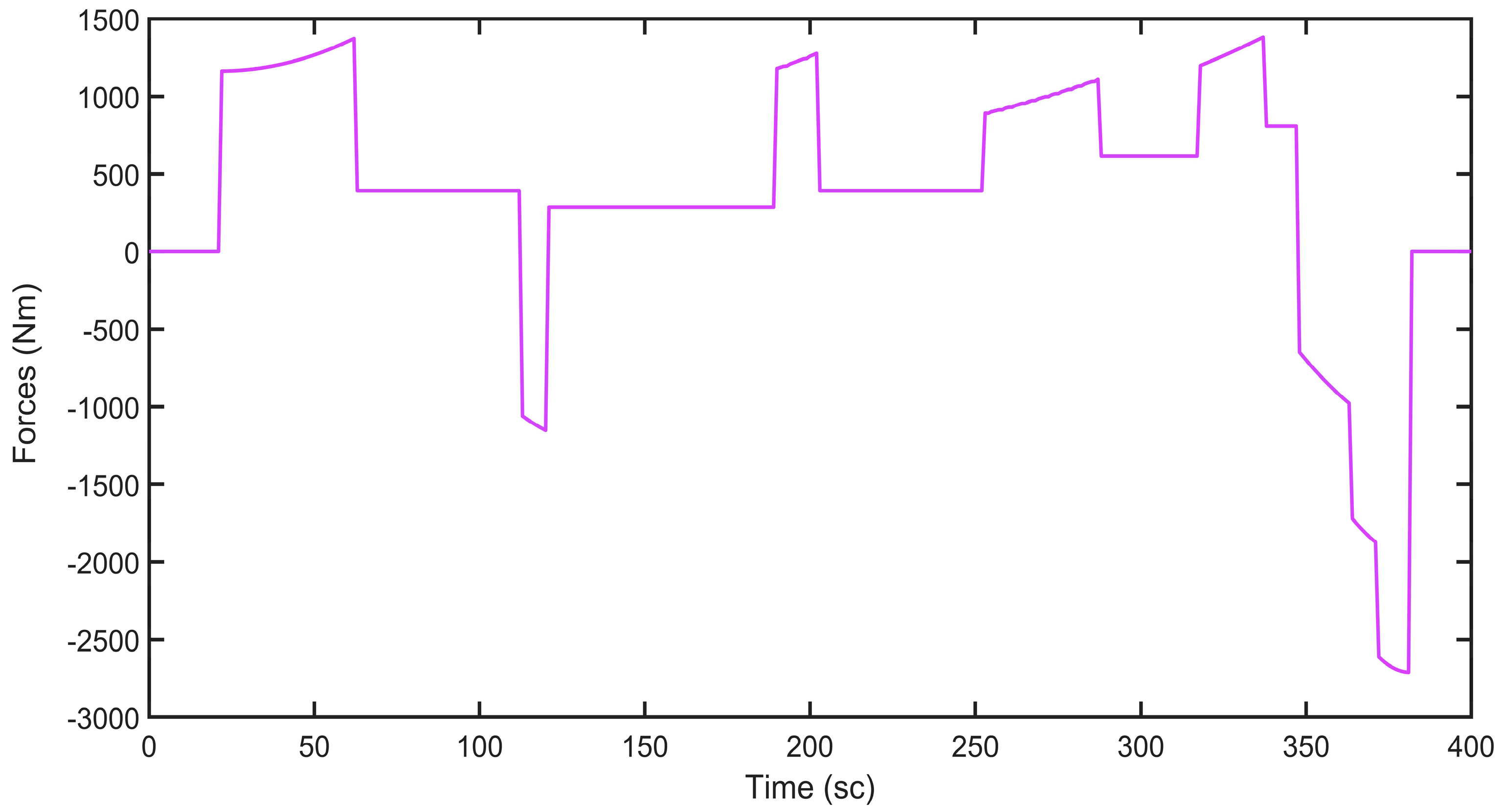
Figure 5 displays the cumulative force exerted on the vehicle, which assists in determining the operational phases of the engines: the internal combustion engine operates when power demand is high, while the electric motor takes over during periods of low power demand.
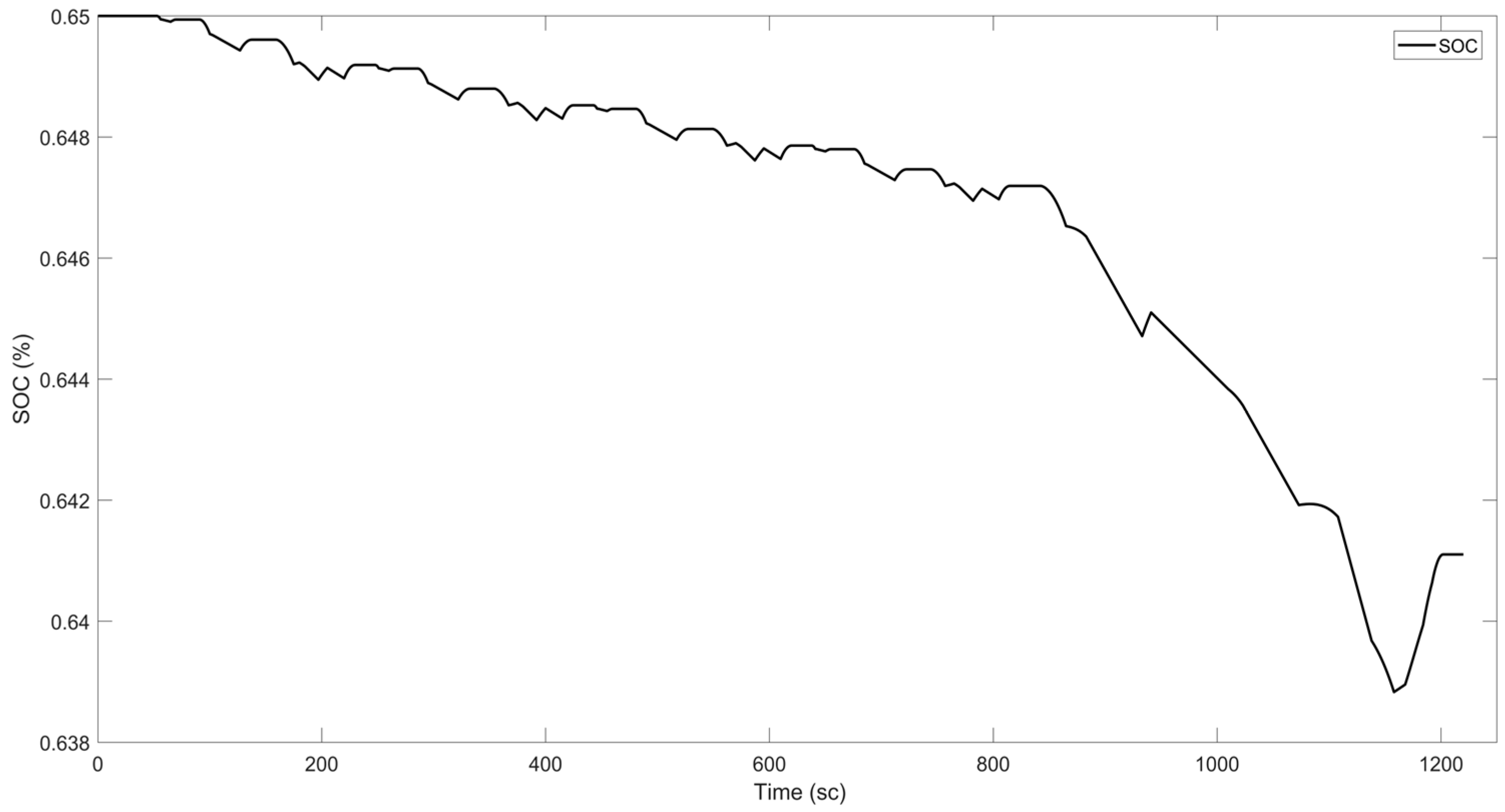
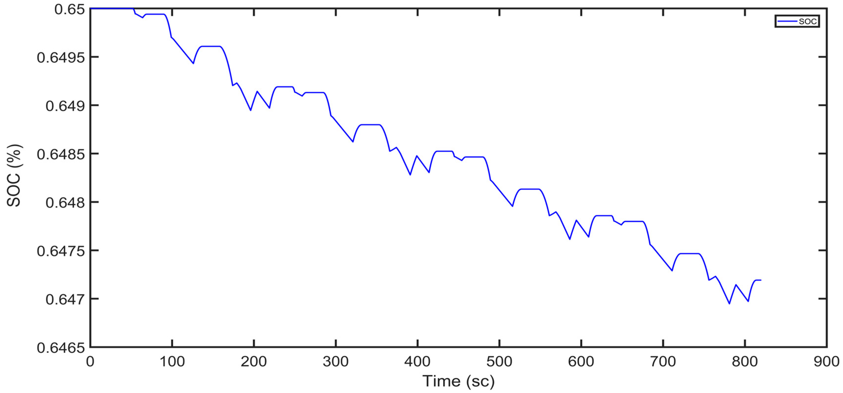
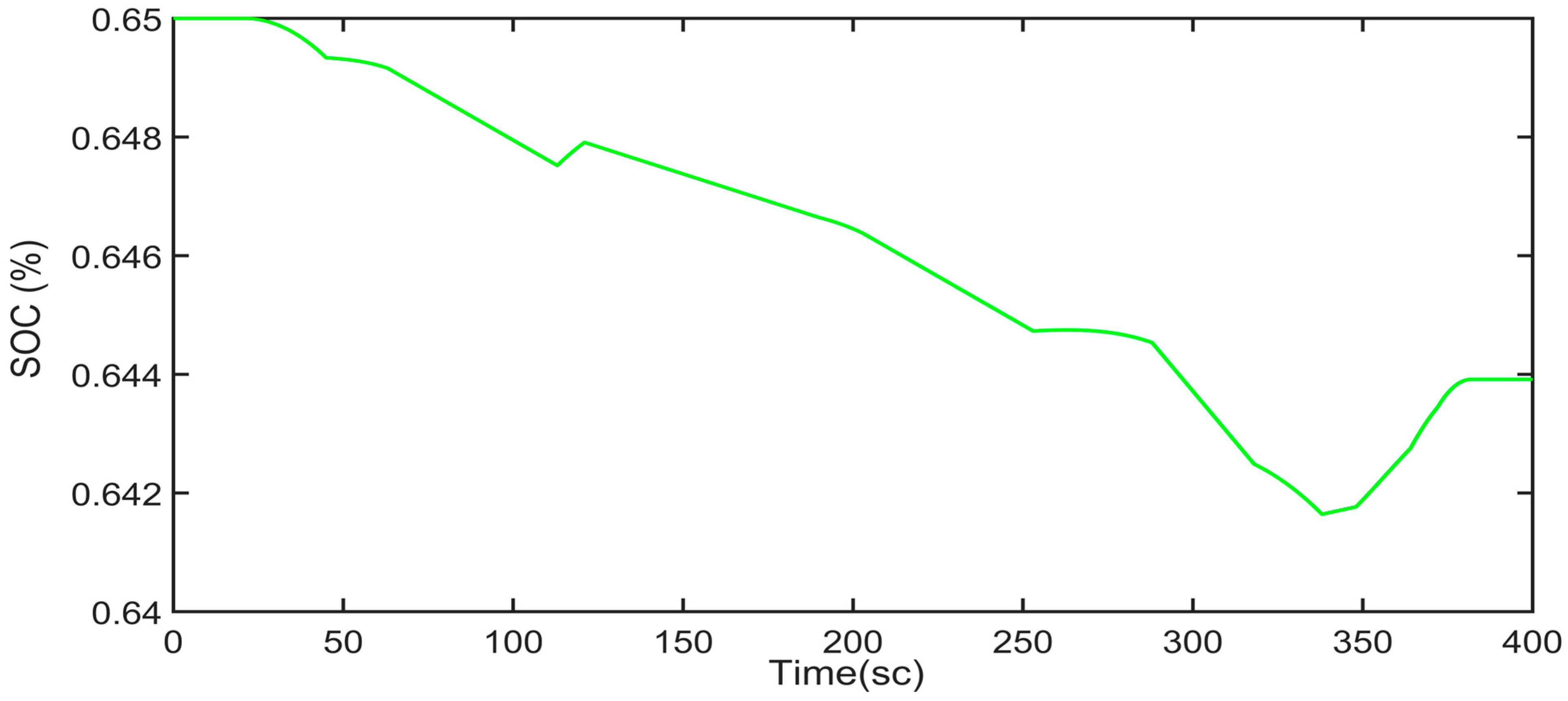
In line with the results obtained from the experimental results, the charge state of the battery according to time is shown in
Figure 6. The parts where the SOC rises indicate that the electric motor is operating as a generator.
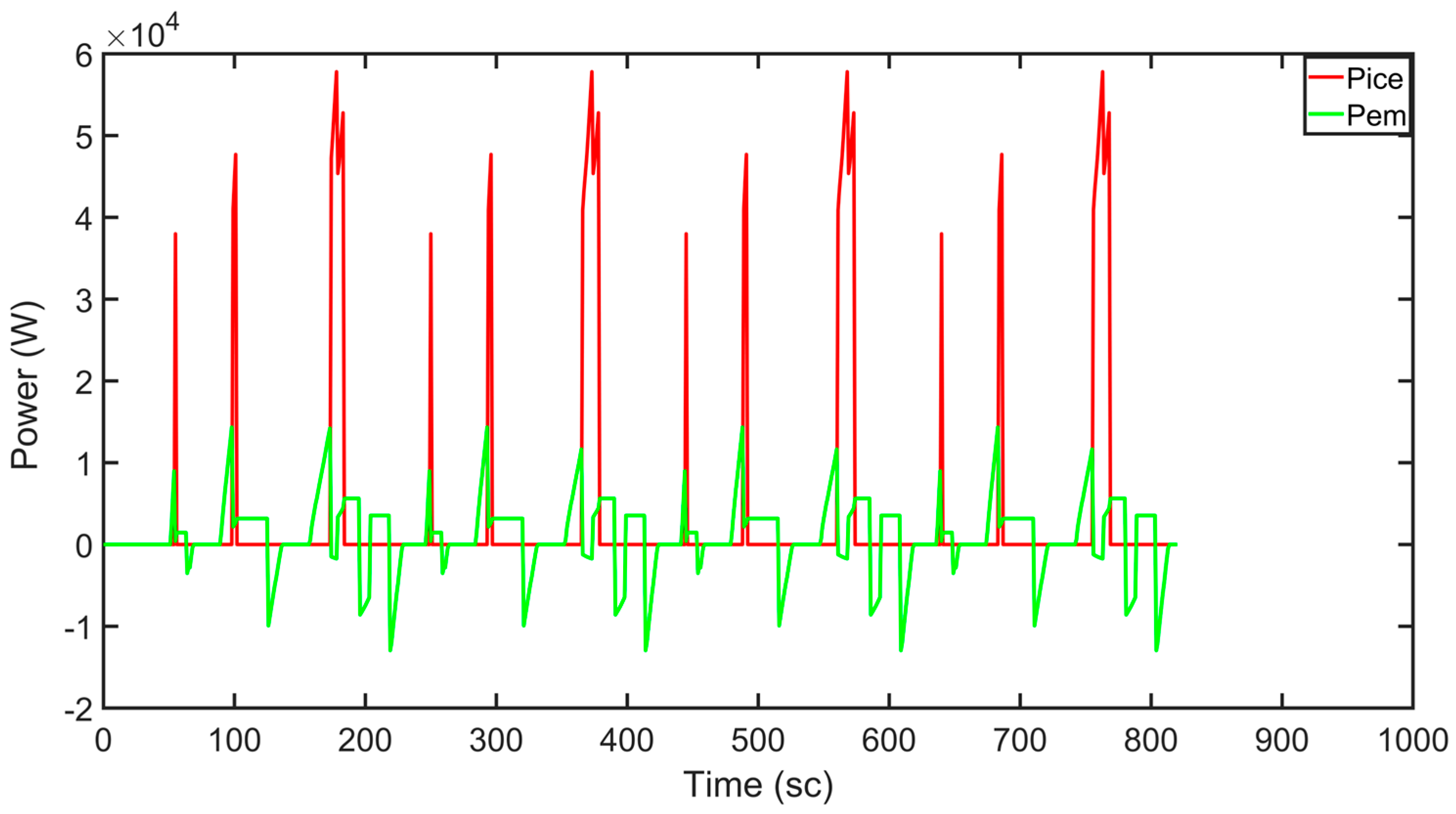
In
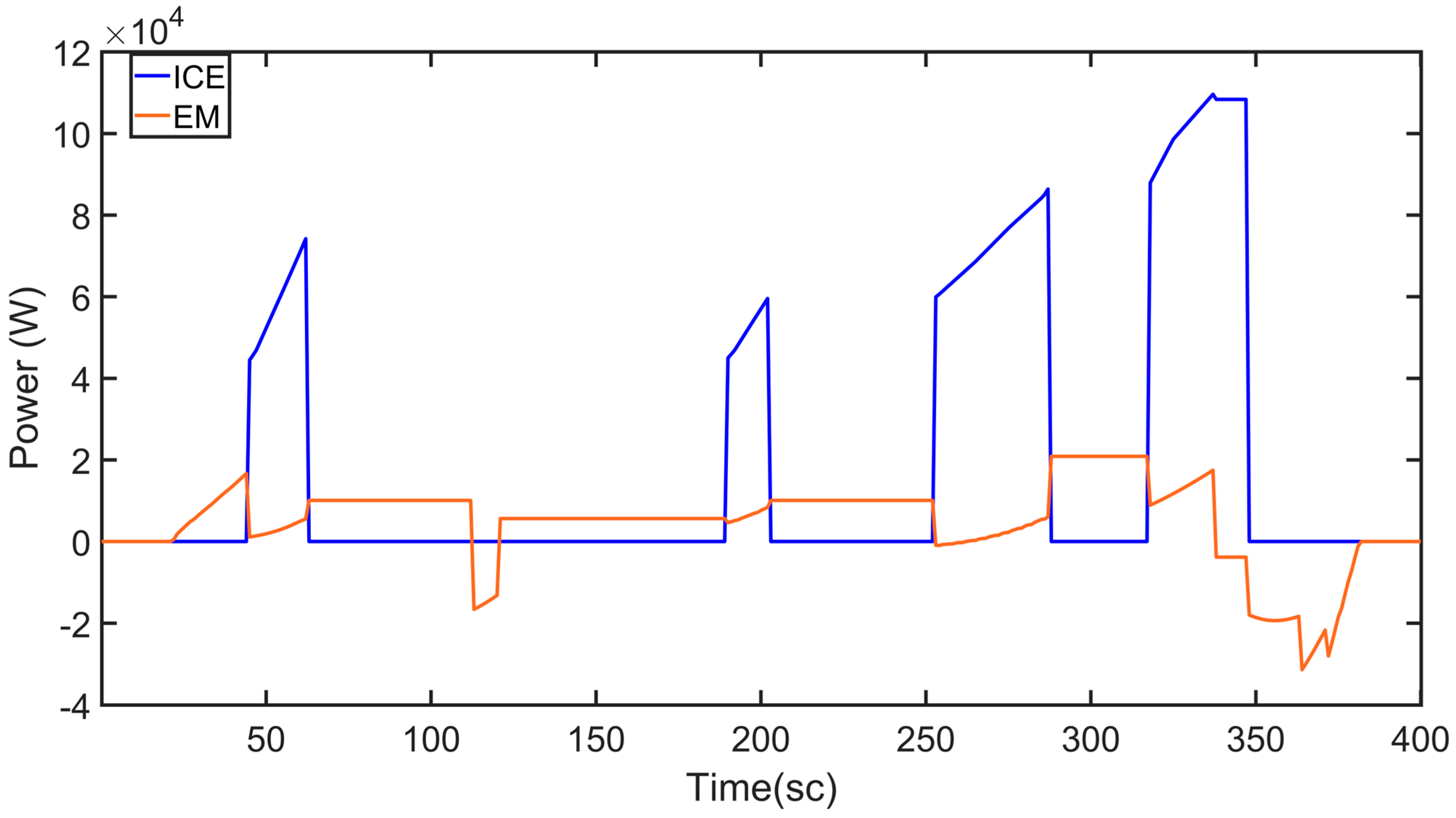
Figure 7, the power levels of both the internal combustion engine and the electric motor are observed during the driving cycle. The internal combustion engine’s power is represented in red, while the electric motor’s power is depicted in black. The negative power of the electric motor signifies its operation as a generator.
In
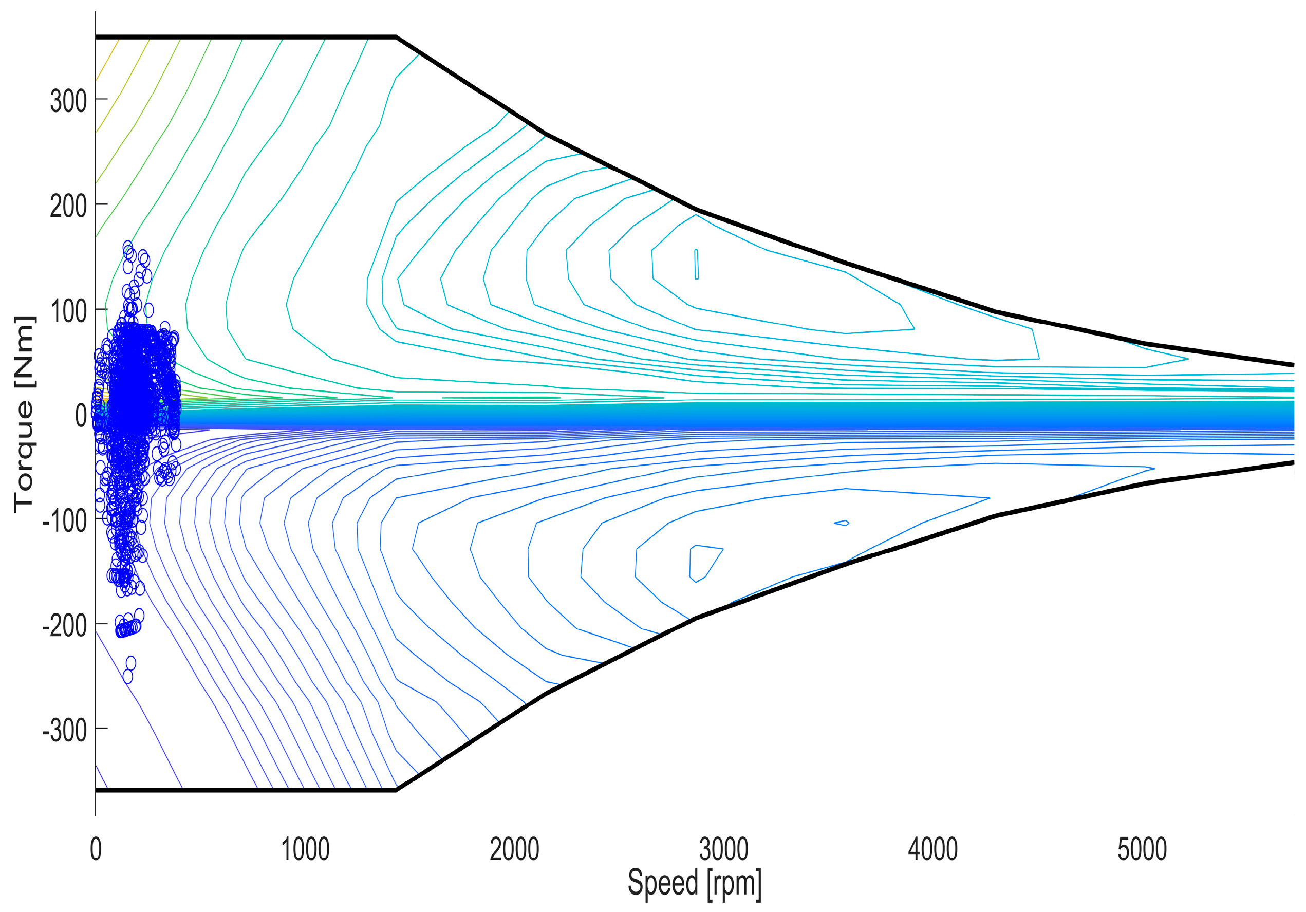
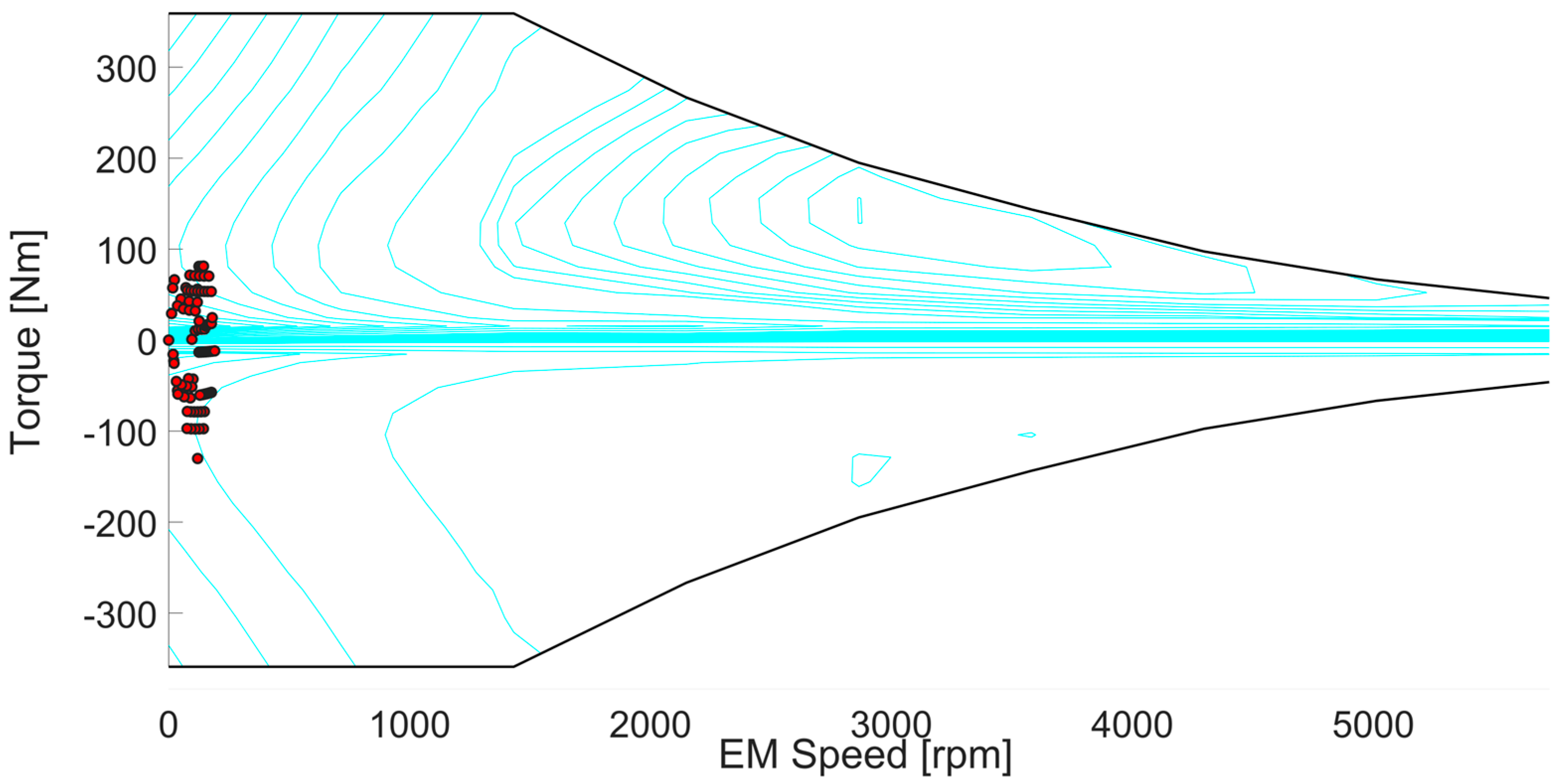
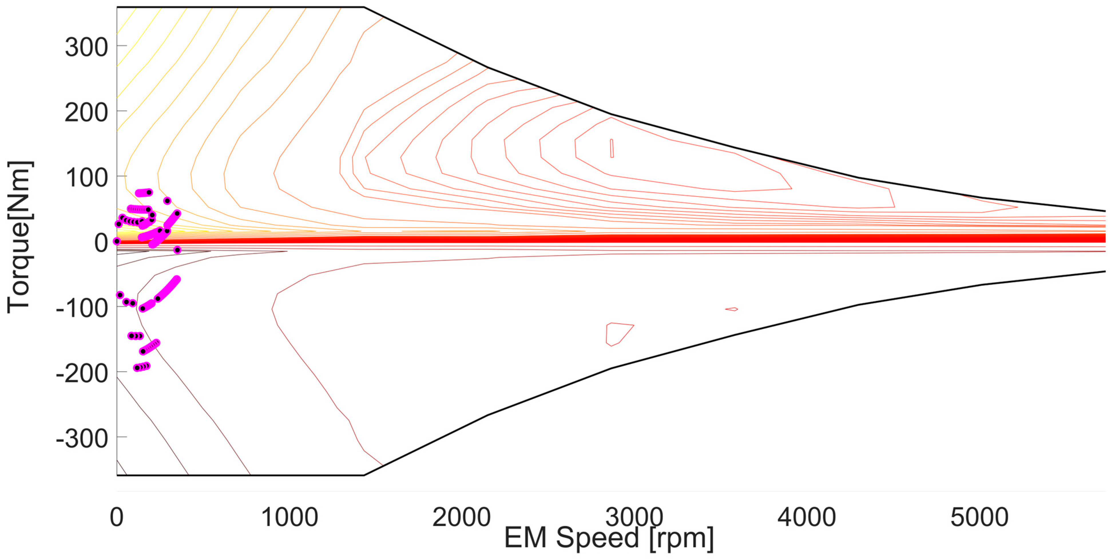
Figure 8, the operating points of the electric motor are shown with a blue dot. The electric motor operates when the speed and torque are low.
Figure 8 shows that the electric motor operates in efficient regions and frequently. The clustering of EM in the loops where low power is required indicates that the control method system is working correctly because the vehicle is operating at low power in the control system. In addition,
Figure 8 shows that the electric motor produces too much negative torque, so it shows that the EM is working as a generator.
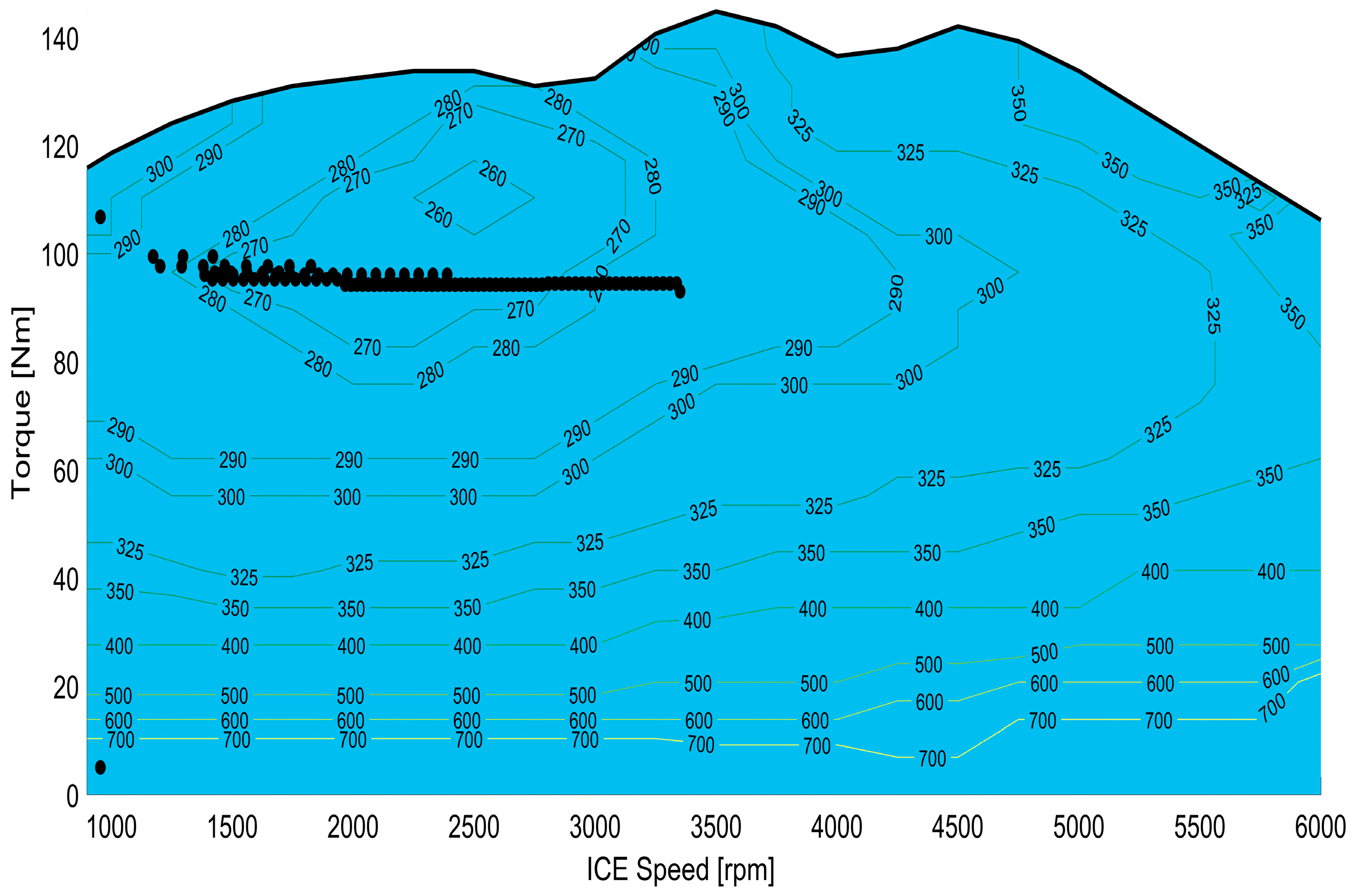
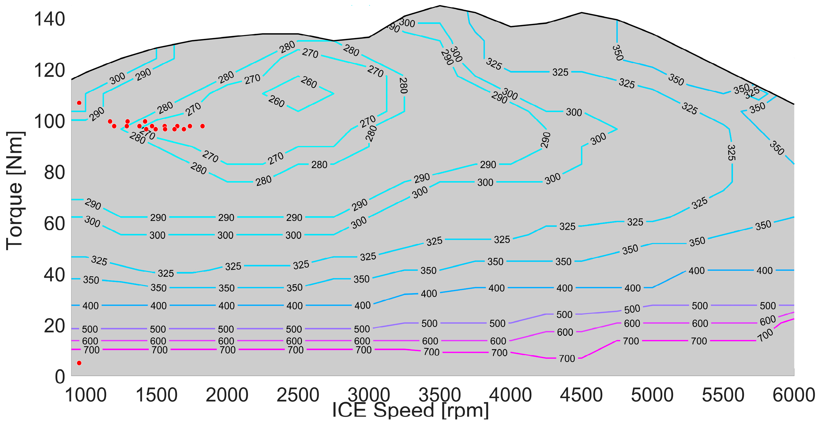
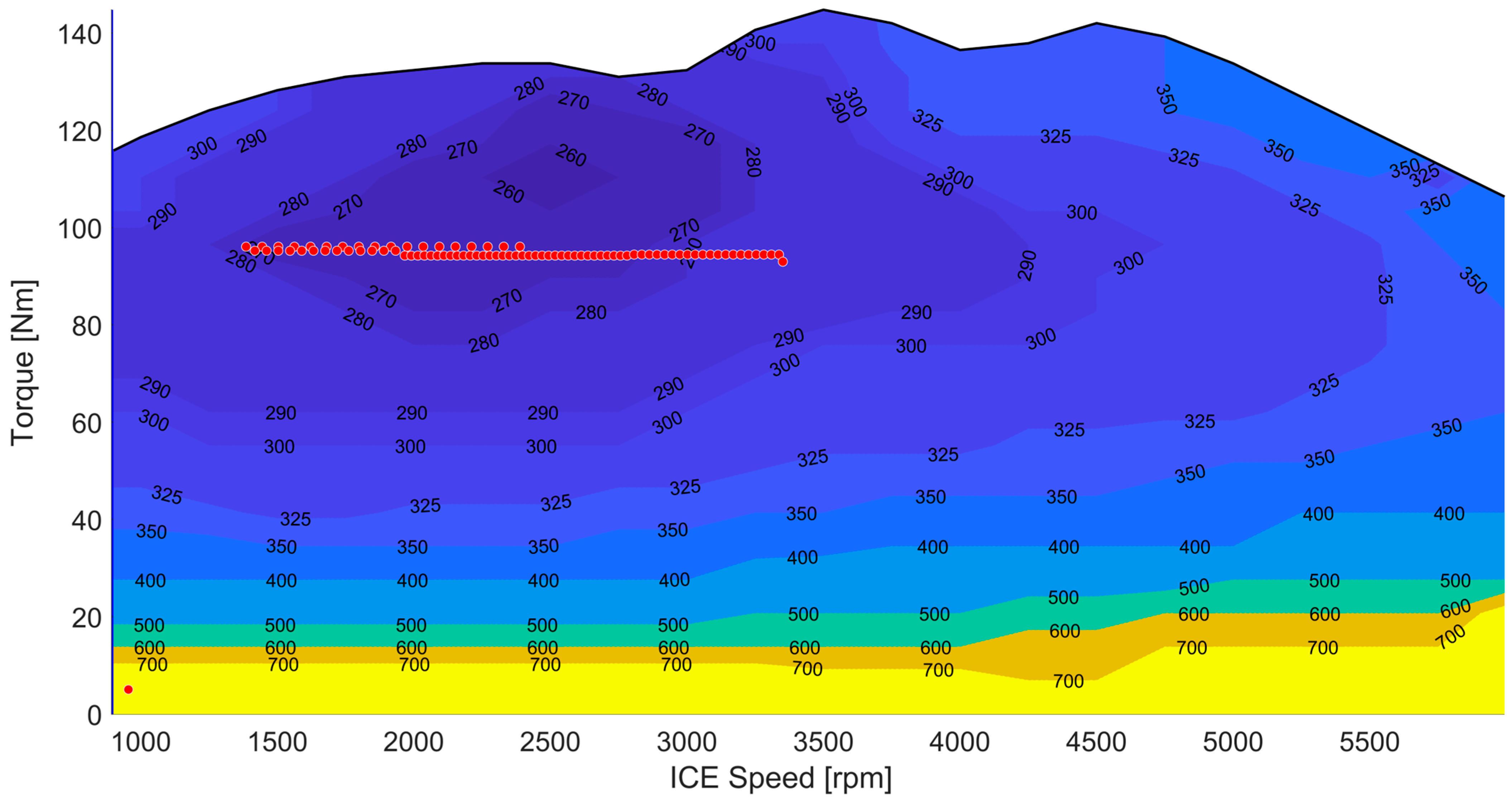
The specific fuel consumption of the internal combustion engine is shown in
Figure 9. The black dots clustered in
Figure 9 represent the value of fuel in grams when the internal combustion engine is running. When
Figure 9 is carefully examined, it is seen that the fuel is fixed at the lowest points.
The results obtained from the utilization of the machine learning algorithm, in combination with the recommended control strategy, are displayed in
Figure 10,
Figure 11,
Figure 12,
Figure 13 and
Figure 14 for the ECE-15 cycle. In
Figure 10, the total force applied to the vehicle is illustrated, aiding in identifying the operational phases of the engines. The internal combustion engine functions during periods of high power demand, whereas the electric motor takes charge during periods of low power demand.
The change of the battery over time in the ECE-15 driving cycle is shown in
Figure 11. Due to the low speed and power values inherent in the ECE-15 driving cycle, it is seen in
Figure 11 that the energy increase is very small.
Figure 12 illustrates the power generated by the rule-based control method during the ECE-15 driving cycle for both the internal combustion engine and the electric motor. Upon closer examination of
Figure 12, it becomes apparent that the internal combustion engine (ICE) produces more power with an increase in vehicle speed. Given the low-speed value in the ECE-15 cycle, the electric motor (EM) operates more prominently. The power value of the electric motor exhibits constant fluctuations in
Figure 12, indicating that the rule-based control algorithm enables the electric motor to operate efficiently at low power demands. Additionally, the negative power in
Figure 12 suggests that some of the power generated by the internal combustion engine, after operating at high power, is transmitted to the electric motor, allowing it to function as a generator. In this context, it demonstrates that the electric motor (EM) is responsible for charging the battery. The operational points of the electric motor are illustrated in
Figure 13. Upon closer examination of
Figure 13, it becomes evident that the electric motor consistently operates in efficient regions.
This is attributed to the low speed and torque values in the ECE-15 cycle, which includes the urban cycle. The fuel consumption, measured in grams, when the internal combustion engine (ICE) is in operation is depicted in
Figure 14. The red dots in
Figure 14 represent the grams of fuel consumption during ICE engine operation. It is observed that these red dots are concentrated at the most optimal and lowest points, indicating that the ICE engine is used less frequently.
The rule-based energy control management algorithm for the EUDC driving cycle is employed, and the simulation results are analyzed. In
Figure 15, the cumulative force exerted on the vehicle is depicted, assisting in the identification of the operational phases of the engines. Specifically, the internal combustion engine operates during periods of high-power demand, while the electric motor takes over during intervals of low power demand.
Figure 16 illustrates the temporal variation of the State of Charge (SOC) using the energy control method in the EUDC cycle. When analyzed in
Figure 16, the battery has decreased to 64.4% due to the high power demanded. This reduction indicates that maximum speed and torque values are used. The power generated by the internal combustion engine (ICE) and electric motor (EM) according to the rule-based control method in the EUDC driving cycle is depicted in
Figure 17. It is evident that the ICE power in the EUDC cycle, characterized by high-speed values, surpasses that in the ECE-15 cycle.
In
Figure 18, the operating points of the EM are illustrated with purple dots. When
Figure 18 is examined, it is observed that the electric motor works less in efficient regions compared to the ECE-15 cycle. The reason is that the EUDC cycle includes the extra-urban cycle, so the speed and torque values are high. In addition, it is seen that the negative power point is higher in
Figure 18 because EM is used as a generator since it is high power. The gram value of the fuel used when the ICE engine is running is shown in
Figure 19.
In this study, fuel consumption estimation is planned for a dataset that includes the rule-based control method. Fuel consumption prediction are evaluated using two distinct test data ratios, such as 1.7% and 25%. Evaluation and validation of a model are important steps that allow the determination of the extent to which the prepared model achieves the presumptive goal. In this context, linear regression, random tree, random forest, decision log, M5P, REP Tree, and multilayer perceptron methods were used in WEKA 3.8.6 software to determine the best fuel consumption prediction. The effectiveness of machine learning algorithms is evaluated using performance criteria. Correlation Coefficient (
), Root Mean Square Error (
RMSE), and Mean Absolute Error (
MAE) values are used as performance criteria. All performance criteria are given as
where,
,
,
denote the desired output, the predicted output, and the average value, respectively, and
n is the number of samples.
The performance criteria values utilized to evaluate the efficacy of machine learning algorithms are presented in
Table 2 for the 1.7% test data. When
Table 2 is examined in terms of
, the random forest algorithm has the highest value of
which is 0.9716. After the random forest algorithm, the highest
values are REP Tree and M5P, respectively. The lowest
values are Linear Regression, decision stump, and multilayer perceptron which have the lowest values of
. Since the
value is closer to 1 in the random forest algorithm, the prediction accuracy is higher than in the other algorithms.
When
Table 2 is analyzed in terms of MAE, the highest error value is observed in the multilayer perceptron, and the lowest error value is observed in the random forest algorithm. Moreover, the REP Tree and M5P algorithms have almost the same MAE value.
Considering the RMSE value in
Table 2, as in MAE, it is seen that the largest error value is multilayer perceptron, and the smallest error is random forest algorithm. Although the RMSE of the M5P algorithm and the RMSE of the REP Tree algorithm are close, the RMSE of the REP Tree algorithm is the second-lowest error. The M5P algorithm has the third-lowest error in terms of RMSE. Moreover, the RMSE values of the decision stump and linear regression algorithms are close to each other.
The performance criteria values utilized to evaluate the efficacy of machine learning algorithms are presented in
Table 3 for the 25% test data. When
Table 3 is examined in terms of
, the random forest algorithm has the highest value of
which is 0.9021. After the random forest algorithm, the highest
values are Random Tree and REP Tree, respectively. The lowest
values are decision stump, M5P, and linear regression, which have the lowest values of
.
When
Table 3 is analyzed in terms of MAE, the highest error value is observed in the linear regression and the lowest error value is observed in the random forest algorithm. Moreover, the Random Tree and REP Tree algorithms have almost the same MAE value.
Examining the RMSE value in
Table 3, akin to MAE, reveals that the largest error value is linear regression, and the smallest error is the random forest algorithm. In addition, the Random Tree and REP Tree algorithms have the same values, which are the second lowest error.
When the results in
Table 2 and
Table 3 are analyzed according to both test data, they show that the random forest algorithm techniques can provide sufficient fuel consumption prediction for the parallel hybrid electric vehicle in this study.
Simulation results of fuel consumption that are obtained using machine learning algorithms are shown in
Figure 20,
Figure 21,
Figure 22,
Figure 23,
Figure 24,
Figure 25 and
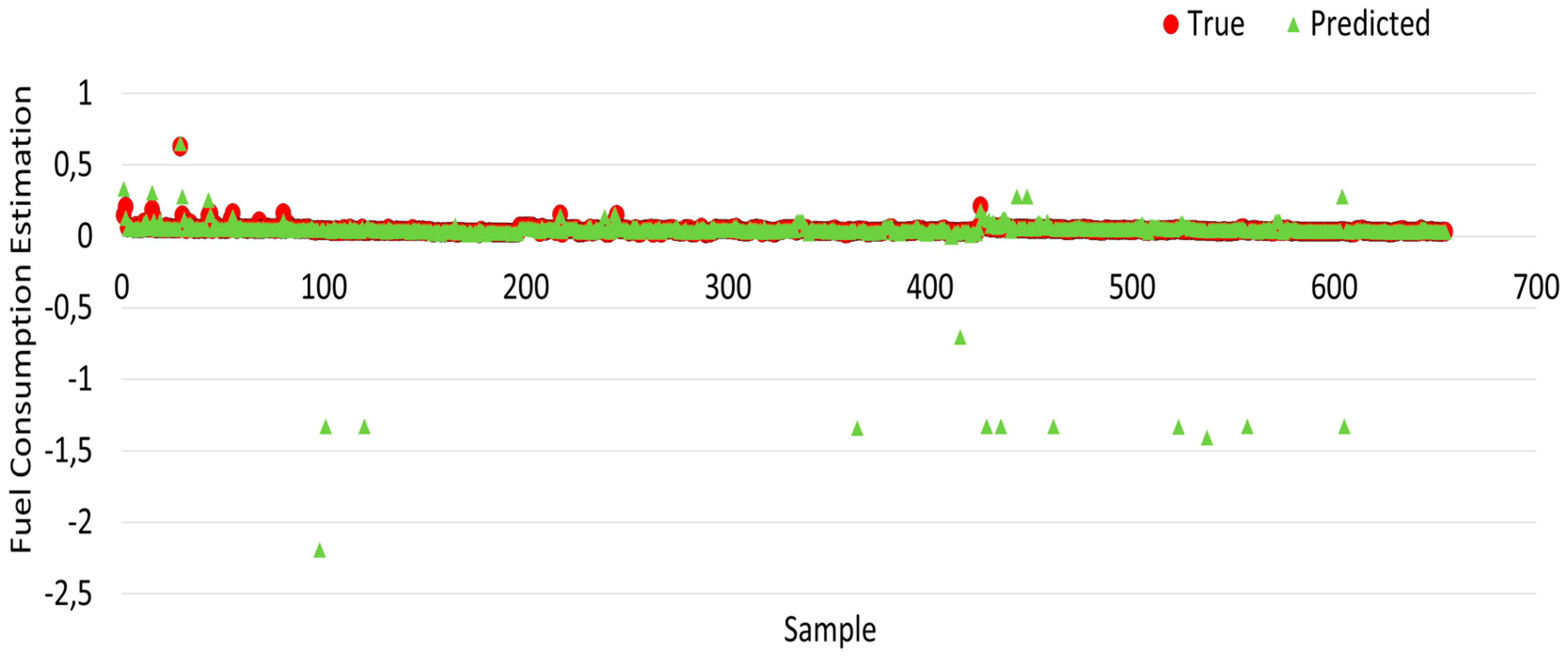
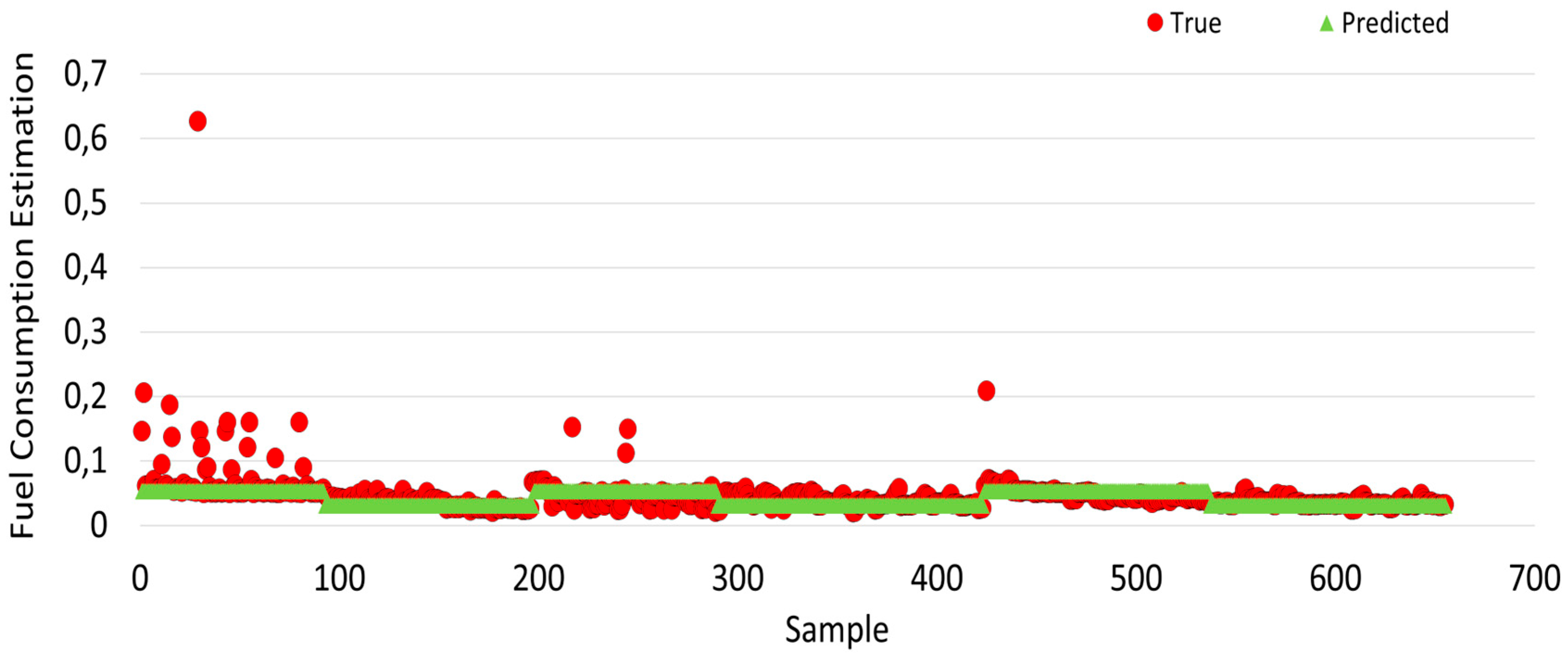
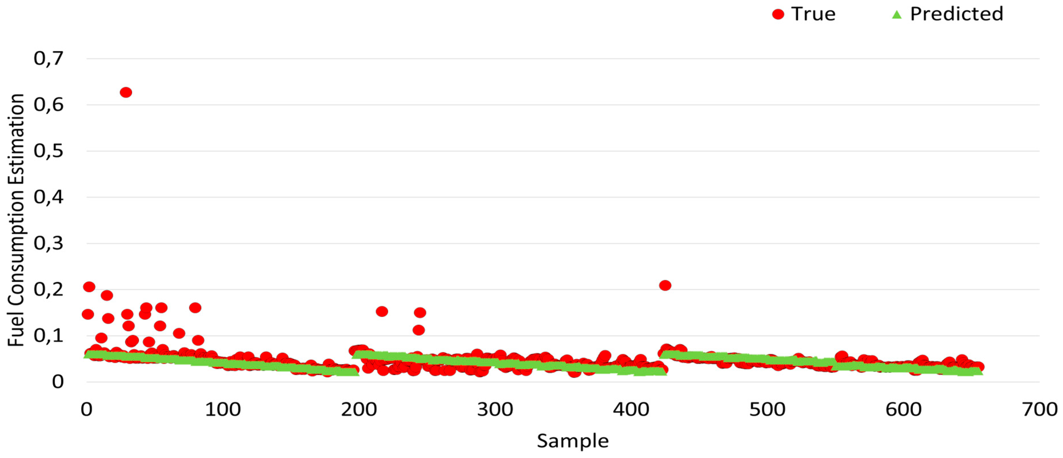
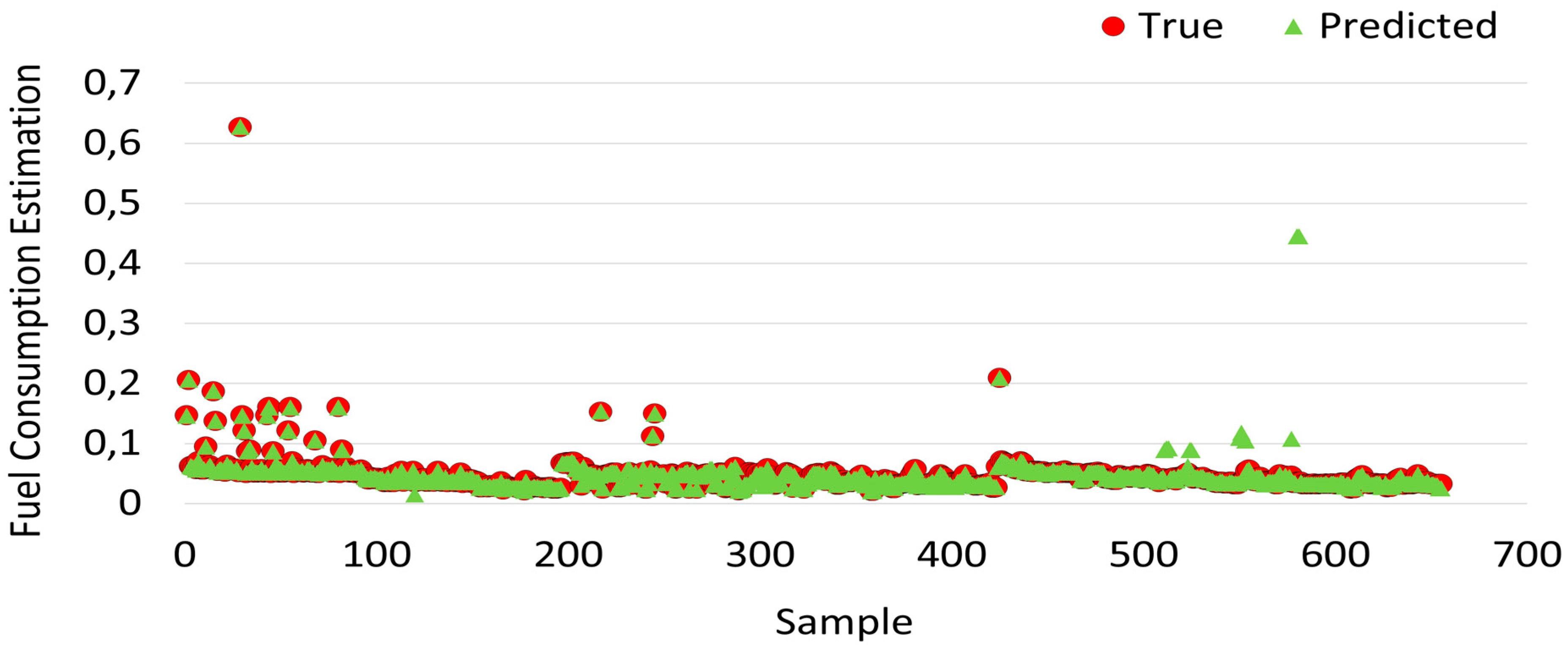
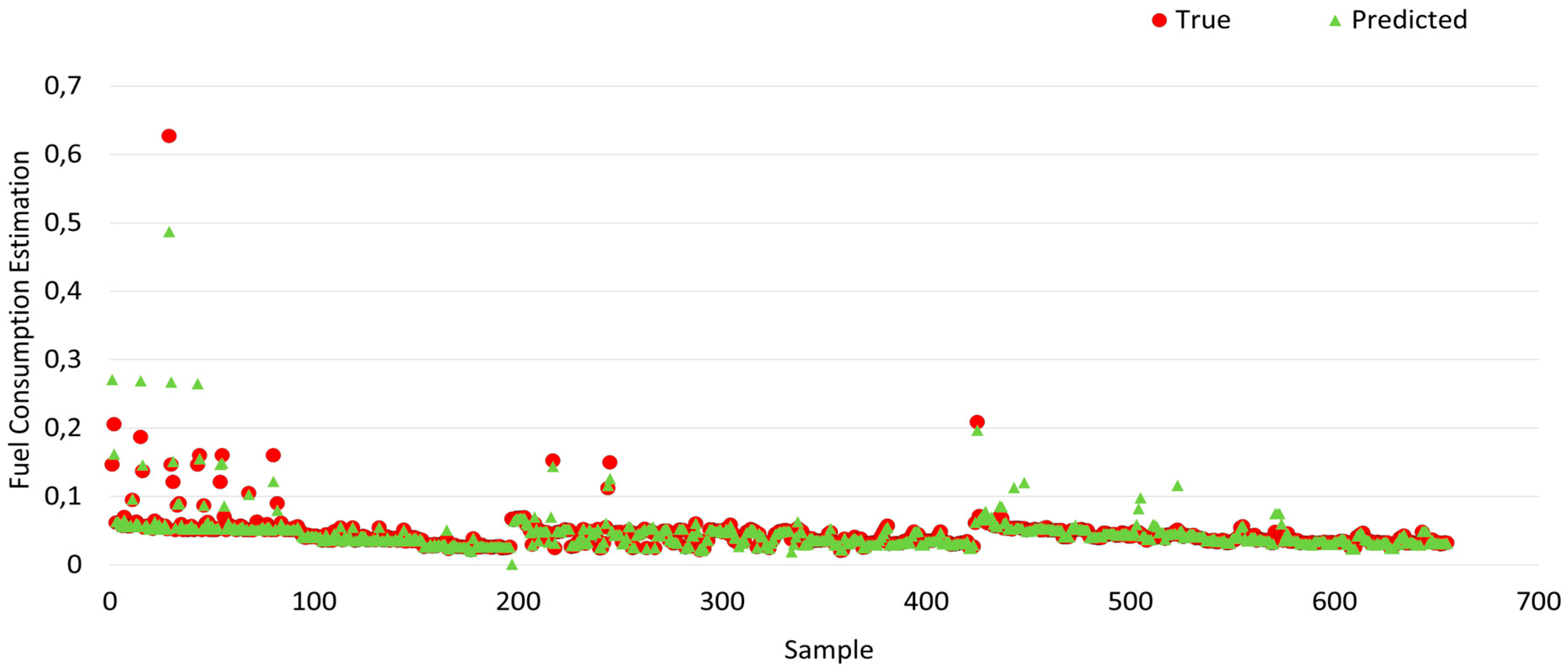
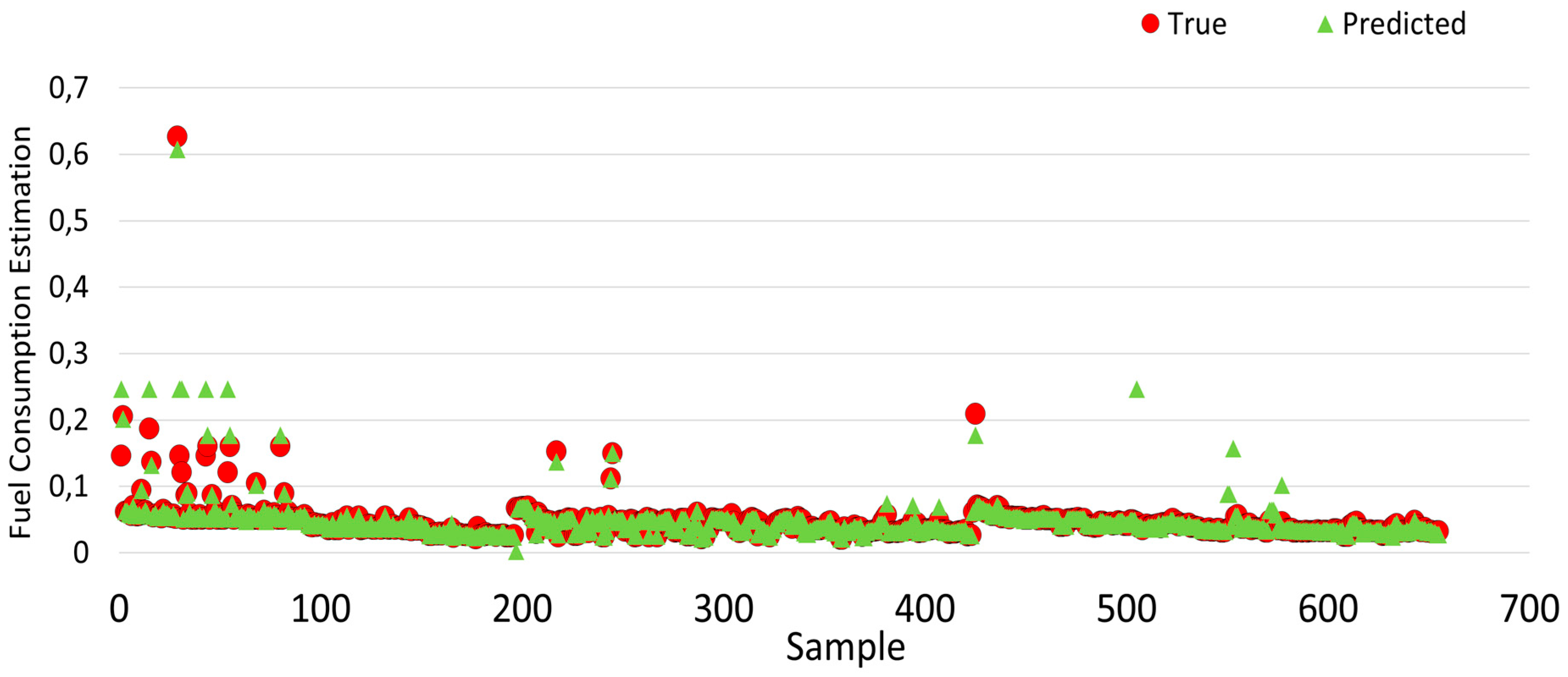
Figure 26. Due to the volume of data in the 25% test data, it is impractical to plot the graph of actual values against predicted values. Therefore, the simulation results are reflective of the values obtained from the 1.7% test data. In
Figure 20,
Figure 21,
Figure 22,
Figure 23,
Figure 24,
Figure 25 and
Figure 26, the actual values obtained from the experiment are shown as red circles, while the predicted values are shown as green regions.
The predicted values of the multilayer perceptron prediction result are given in
Figure 20. It is observed that the estimated values did not fully match the actual values in
Figure 20 because of the significant difference in error between the predicted values and the actual values.
The predicted values of the decision stump algorithm are illustrated in
Figure 11. The fact that the predicted values as a result of the decision stump algorithm are higher in
Figure 21 indicates that the error value is high.
The predicted values obtained because of linear regression with the actual value are given in
Figure 22. As the error value is high in the prediction result with linear regression, the actual values and the predicted values do not match.
The fuel consumption prediction of the random tree algorithm is shown in
Figure 23, which shows that the actual values and the predicted values coincide. Hence, the error is less.
The prediction results of the M5P algorithm are illustrated in
Figure 24, and when
Figure 24 is carefully examined, it is seen that the actual values and the predicted values almost match each other.
The prediction results of the REP Tree algorithm are illustrated in
Figure 25, and it is seen that the error value was the lowest after the random tree and M5P algorithms.
Finally, the prediction results of the random forest algorithm are given in
Figure 26. When
Figure 26 is examined, it is almost identical to the estimated and actual values based on the training results. Therefore, it has been observed that random forest algorithms make better predictions.
The hyperparameters of the machine learning algorithms are selected by default in the Weka 3.8.6 program. The goal of choosing the default settings is to guarantee an equitable comparison between algorithms without the need to set any particular parameters. The batch size, which is a hyperparameter of the machine learning algorithms, is set to 100. The hyperparameters of the Multilayer Perceptron encompass learning rate and momentum, with values set at 0.3 and 0.2, respectively. In addition, the minimum proportion of the variance on all the data that needs to be present at a node in order for splitting to be performed in a regression tree is set to 0.01 for the Random Tree algorithm. Furthermore, the random number seed used for selecting attributes is set to 1 for the Random Tree, REP Tree, and Random Forest algorithms. The amount of data used for pruning are set to 3 in the Rep Tree algorithm. Moreover, the number of execution slots (threads) to be used to create the community is set to 1 in the Random Forest algorithm.
The computation times of machine learning algorithms are given in
Table 4 for 1.7% of the test data. It can be seen from
Table 4 that the Decision Stump algorithm is faster than other algorithms. In addition, the multilayer perceptron algorithm has the slowest computation time. Although the random forest model provides the most accurate predictions of fuel consumption, it has the second slowest computation time for 1.7% of the test data.
The computation times of machine learning algorithms are given in
Table 5 for 25% of the test data. It can be seen from
Table 5 that the Decision Stump algorithm is faster than other algorithms. Moreover, the multilayer perceptron algorithm has the slowest computation time. While the random forest model delivers the most precise fuel consumption predictions, it ranks as the second slowest in terms of computation time for the 25% test data.
This article examines fuel consumption estimation using machine learning methods with rule-based control methods. According to the results obtained, the vehicle consumes 4.72 Lt/100 km of fuel with the proposed method, while the gasoline-fueled vehicle consumes 7 L per 100 km. Therefore, the proposed method reduces 4.69 kg of CO
2 emissions. In addition, the fuel consumption value obtained in [
22] is 5.4 L/100 km. Our proposed method produces less carbon emissions compared to [
22].
5. Conclusions
In this article, a control algorithm was created with the goal of minimizing carbon emissions through the efficient prediction of fuel consumption and optimized utilization of energy resources. The primary objective of this research is to decrease carbon emissions by forecasting fuel consumption and enhancing the efficiency of energy resource utilization. Therefore, a new dataset is generated through experimentation in driving cycles to estimate fuel consumption in a parallel hybrid electric vehicle, utilizing a rule-based control algorithm. In the literature, only road information is taken as an input value for fuel consumption and, prediction. In this study, the new dataset consists of 11 different input values and 1 output value. The dataset contains 11 inputs and 1 output. Inputs are EM speed, EM torque, EM power, ICE speed, ICE torque, ICE power, driving cycle speed, driving cycle acceleration, torque, Forces, and SOC. The output is fuel consumption. In addition, the dataset includes a rule-based control method, which allows the internal combustion engine to operate at an optimal level and the electric motor to work both as a generator and to move the vehicle up to a certain speed under the required conditions. Train and test data were carried out for seven distinct machine learning methods using normalized training data. In this study, a test data set were produced by concealing the projected fuel amount in the original data set. Each technique looks at the fuel consumption numbers whose regression is required in the test and uses the weight coefficients learned through training to provide the best appropriate prediction value. Furthermore, during the testing phase, both 1.7% and 25% of the entire dataset were employed to assess the accuracy of fuel consumption estimation. Using machine learning methods, the fuel consumption accuracy estimates were found to be 97.16%, 94.2%, 93.54%, 91.58%, 16%, 81.3%, and 80.36% for the random forest algorithm, the REP Tree algorithm, the M5P algorithm, the random tree algorithm, the multilayer perceptron algorithm, the linear regression algorithm, and the decision stump algorithm, respectively, for 1.7% of the test data. In addition, the random forest algorithm exhibited a remarkable accuracy of 90% for the 25% test data, surpassing the performance of other algorithms. According to the results, the Random Forest algorithm was the most appropriate method in terms of training and testing the fuel consumption model for a parallel hybrid electric vehicle in this study. Moreover, the vehicle’s fuel consumption using the proposed approach stands at 4.72 L per 100 km, in contrast to the gasoline-powered vehicle’s consumption of 7 L per 100 km based on the results.
Due to the frequent use of the electric motor in hybrid vehicles, there are fluctuations in the calculation of CO2 emissions. This can lead to a miscalculation of fuel consumption and carbon emissions. It has been shown that the fuel consumption for the vehicle used in this study can be predicted quickly and accurately under different conditions without the need for time-consuming vehicle tests, fuel consumption, or even carbon emissions to the atmosphere due to fuel consumption. Thanks to the proposed method, fuel consumption estimation can be conducted accurately with the random forest algorithm method. With the knowledge and methodology gained from this study, similar studies can be conducted for different vehicles. In addition, such studies would make it easy to determine fuel consumption even before hybrid vehicles are produced.
In future studies, it is considered necessary to further improve the data set by considering traffic congestion. Moreover, metaheuristic algorithms will be used with deep learning to fine-tune hyperparameters.

