Article

Scalable Inverse Uncertainty Quantification by Hierarchical Bayesian Modeling and Variational Inference

1
Department of Nuclear, Plasma and Radialogical Engineering, University of Illinois at Urbana Champaign, Champaign, IL 61820, USA
2
Department of Nuclear Engineering, North Carolina State University, Raleigh, NC 27695, USA
*
Author to whom correspondence should be addressed.
Energies 2023, 16(22), 7664; https://doi.org/10.3390/en16227664
Submission received: 22 September 2023 / Revised: 17 November 2023 / Accepted: 17 November 2023 / Published: 20 November 2023
(This article belongs to the Section B4: Nuclear Energy)

Abstract

:
Inverse Uncertainty Quantification (IUQ) has gained increasing attention in the field of nuclear engineering, especially nuclear thermal-hydraulics (TH), where it serves as an important tool for quantifying the uncertainties in the physical model parameters (PMPs) while making the model predictions consistent with the experimental data. In this paper, we present an extension to an existing Bayesian inference-based IUQ methodology by employing a hierarchical Bayesian model and variational inference (VI), and apply this novel framework to a real-world nuclear TH scenario. The proposed approach leverages a hierarchical model to encapsulate group-level behaviors inherent to the PMPs, thereby mitigating existing challenges posed by the high variability of PMPs under diverse experimental conditions and the potential overfitting issues due to unknown model discrepancies or outliers. To accommodate computational scalability and efficiency, we utilize VI to enable the framework to be used in applications with a large number of variables or datasets. The efficacy of the proposed method is evaluated against a previous study where a No-U-Turn-Sampler was used in a Bayesian hierarchical model. We illustrate the performance comparisons of the proposed framework through a synthetic data example and an applied case in nuclear TH. Our findings reveal that the presented approach not only delivers accurate and efficient IUQ without the need for manual tuning, but also offers a promising way for scaling to larger, more complex nuclear TH experimental datasets.

1. Introduction

Computer simulations play an essential role in nuclear reactor safety analysis, design, and licensing. While these simulations can model real physical phenomena, they are approximations with inherent uncertainties from various sources. Quantifying these uncertainties is an important step in the simulation model validation process because the assessment of model accuracy requires a reliable measure of uncertainty for model predictions. Uncertainty quantification (UQ) is the process of quantifying the uncertainties in the model outcomes (Quantities-of-Interest, or QoIs) by propagating the uncertainties from the input parameters through the computer model. In the nuclear energy community, UQ holds a particularly pivotal role, compared to other field, as it aids in minimizing over-conservatism in systems with potentially severe consequences. Key activities in nuclear power plant development, such as nuclear reactor design, safety analysis, and licensing, all rely on computer codes whose credibility has been established through a rigorous verification, validation and uncertainty quantification (VVUQ) process.
Inverse Uncertainty Quantification (IUQ) is the process of inversely quantifying the input uncertainties based on experimental data. IUQ seeks statistical descriptions of the uncertain input parameters that are consistent with the experimental data [1]. The uncertainty information of the input parameters can thus be used for further VVUQ tasks. IUQ has emerged as a particularly prominent segment of UQ in recent years, which can be attributed to the increasing requirements from using computer codes for nuclear reactor simulations, as well as the continuous expansion in computational power, coupled with advancements in machine learning and sophisticated statistical methodologies.
A comprehensive framework for computer model calibration under the Bayesian formulation was initially introduced by Kennedy and O’Hagan [2]. Subsequently, this methodology has been adapted for use in various domains. While the technique offers a broad framework for implementing Bayesian calibration in computational models, it requires customization for specific fields. Because the method is dependent on the available measurement data and the parameter space, which are very different across different domains. IUQ is a natural extension to Bayesian calibration because instead of calibrating the input parameters with a point estimate, it primarily focuses on the distribution information of input parameters. In the nuclear TH field, IUQ has primarily focused on the parametric uncertainty from closure relations in TH codes.
Parametric uncertainty can come from the empirical equations used in two-fluid models or other fluid dynamics models, like equations of state and constitutive equations (also known as closure laws). These model parameters are not always known precisely. For large-scale modeling, two-phase transport phenomena are usually described with a multi-fluid continuum formulation and a system of mass, momentum, and energy conservation equations derived for each phase. On smaller scales, complex interactions like forces between phases, evaporation at walls, and others, are typically approximated using various empirical or semi-empirical closure models. The precision and reliability of model predictions largely depend on how well these closure models are calibrated, a process that is traditionally carried out step-by-step. Initially, empirical or semi-empirical submodels undergo calibration and validation using separate-effect test (SET) data, after which the entire model is validated against integral-effect test (IET) data [3]. SETs, commonly executed at a scale smaller than real reactors, primarily concentrate on specific experimental QoIs, minimizing the interference with other phenomena [4]. After thorough analysis of these tests, thermal-hydraulic experts determine the closure relationships. During this procedure, closure models are developed to minimize added computational load. However, these models might possess considerable uncertainties from knowledge gaps, scalability concerns, and oversimplifications.
In recent years, many IUQ methodologies have been developed in the nuclear community and several international projects have also been performed. For example, (1) the PREMIUM (Post-BEMUSE Reflood Models Input Uncertainty Methods) [5] benchmark, which focused on core reflood problems to quantify and validate input uncertainties in system TH models, (2) the SAPIUM (Systematic APproach for Input Uncertainty quantification Methodology) [6] project that aimed to develop a systematic approach for input UQ methodology in nuclear TH codes, and (3) the ATRIUM (Application Tests for Realization of Inverse Uncertainty quantification and validation Methodologies in thermal-hydraulics) [7] project that was initiated in 2022 to perform practical IUQ exercises of a demonstration of the SAPIUM approach. Wu et al. [1] conducted a comprehensive survey where twelve IUQ methods for nuclear TH applications are reviewed, compared, and evaluated. More recently, Liu et al. [8] developed a SAM-ML framework for calibration of closure laws in the SAM system code. A nonlinear extension of the CIRCE method was introduced in [4], employing Bayesian inference for IUQ in closure relations of TH codes. This was further expanded to account for multiple experimental groups in [9]. Furthermore, Xie et al. [10] combined IUQ and quantitative validation via Bayesian hypothesis testing to improve the predictive capability of computer simulations. Besides the applications in nuclear energy, the Bayesian approach for IUQ has also been applied to many other fields such as biotechnology [11], geophysics [12], additive manufacturing [13], computational fluid dynamics [14,15], etc.
Many recent advancements in IUQ are attributed to the rapid evolution of ML/AI technologies. These technologies have not only enhanced the accuracy and reliability of simulation models across diverse industries but have also proven effective in addressing numerous complex challenges [16]. They have been successfully applied in various fields such as healthcare [17,18,19], agriculture [20], transportation [21,22,23], clinical studies [24,25], medical imaging [26,27], civil engineering [28], industrial engineering [29,30], etc. The effectiveness of ML/AI methodologies in these domains demonstrates their versatility and offers valuable insights for our IUQ research in the nuclear energy sector.
In the field of Bayesian IUQ studies for nuclear TH, the research focus has primarily been on using single-level Bayesian inference to investigate the posterior distributions of parameters. These approaches have the advantage of being applicable with relatively small datasets. Nevertheless, the posterior distributions derived from these calculations are typically specific to the chosen experimental scenarios. They may change if different datasets are used. In practice, researchers may be more interested in inferring the population distribution of the parameters given complete experimental datasets. The hierarchical Bayesian models can help in applications where observations are organized into distinct groups. In many nuclear TH applications, the physical model parameters (PMPs) may differ across groups, caused by the group effect introduced by experimental data. For example, many PMPs use different constitutive equations at different experimental conditions (boundary conditions, geometries, flow regimes, etc.). These different constitutive equations impose “group” characteristics—the PMPs within a group show similar behaviors because their constitutive equations are be derived from similar separate-effect test (SET), while the PMPs at very different experimental conditions and constitutive equations are likely to have different level of uncertainty and accuracy. Within each group, the “individual” characteristics of PMPs are due to the parametric uncertainties and measurement error in deriving each constitutive equations. Thus, employing single-level Bayesian inference may introduce errors by ignoring the group-level characteristics in the input parameters. Hierarchical models allow for the creation and identification of “hyperparameters” to make sure that both “group” characteristics and “individual” characteristics of PMPs are considered.
The idea of the hierarchical Bayesian model is not new but has not been extensively explored in the nuclear energy community. The CIRCE method [4] employed a hierarchical structure for a nuclear TH application, where a two-level structure is used and each group consists of a single data point. Robertson et al. [31] used a similar structure to aid the calibration of a fuel performance model. However, the power and flexibility of the hierarchical Bayesian model is not fully explored. Wang et al. [32,33] proposed a flexible hierarchical Bayesian model where data observations can be grouped according to their experimental boundary conditions, and conducted a comprehensive comparison between the hierarchical model and the non-hierarchical model. The hierarchical model structure is demonstrated to be less prone to overfitting caused by model discrepancies or outliers, and has the potential to be used for larger sets of experimental data [32].
However, a practical challenge in the hierarchical Bayesian model is the computation cost. As the number of groups increases, the number of parameters to be quantified also increases. Established Markov Chain Monte Carlo (MCMC) methods scale poorly with data size and parameter space, and become prohibitive when the dimension of parameters is very high. The variational inference (VI) method, also called variational Bayesian, provides a more scalable alternative to MCMC sampling and has been widely used in many applications such as Bayesian neural networks [34], where a large number of parameters need to be estimated. In the field of nuclear engineering, a variational Bayesian Monte Carlo (VBMC) method has been utilized for the IUQ of a doped UO2 fission gas release model [35]. The results showed that VBMC has similar accuracy and superior efficiency compared to traditional MCMC sampling methods.
In this paper, we propose to use VI in the hierarchical Bayesian model to improve the scalability of the Bayesian IUQ framework for nuclear TH applications. We will firstly describe the essential steps in the IUQ framework, then introduce the hierarchical Bayesian model, VI, and explain how they are integrated in the Bayesian IUQ framework. The framework is then applied to a demonstrative example using manufactured data, and later a real-world application using the PMPs in a nuclear TH simulation code and BFBT (BWR Full-size Fine-mesh Bundle Test) benchmark experimental data [36]. Both examples involve more than 300 parameters and VI is used for parameter estimation in the hierarchical model. The resulting posterior distributions of PMPs are compared with the results from No-U-Turn sampler (NUTS) sampling methods, and the efficiency benefit using VI is demonstrated. The proposed method shows a promising framework for reducing the IUQ computation burden and scaling IUQ to large datasets.

2. Materials and Methods

2.1. Bayesian IUQ Framework Overview

IUQ is described as the method to inversely quantify the input uncertainty distributions, based on experimental data. It aims to find statistical descriptions of the uncertain input parameters that are consistent with the experimental data. Bayesian IUQ techniques leverage Bayes’ rule for updating existing knowledge following the observation data [37]. Initial understandings of the uncertainties in the PMPs are captured as prior distributions. These priors are subsequently updated to form posterior distributions through a systematic comparison between the model predictions and experimental data. The obtained posterior distributions of PMPs will be useful for future forward UQ and model validation studies, as well as improving the understandings of the underlying physical models.
The key elements of the IUQ framework are illustrated in Figure 1. In this framework,  x  represents control parameters like boundary and initial conditions, while  θ  in this work denotes the PMPs used in the closure models for TH simulation codes whose uncertainties are the target of IUQ. These TH codes, such as TRACE, encompass a set of six conservation equations that are completed using additional closure models  M i ( x , θ , y M ) . The simulation code’s output, denoted by  y M , can be integrated with the experimental data  y E  using Bayes’ rule. This integration yields a joint posterior probability density distribution for the selected PMPs.
Following the seminal work of Bayesian calibration for computer codes [2], we represent the relationship between the computer code outputs  y M ( x , θ )  and the experimental data  y E ( x )  in the following equation:
y E ( x ) = y M ( x , θ ) + δ ( x ) + ϵ ,
where  ϵ  is the experiment measurement error that is usually assumed to be i.i.d Gaussian distributions  N ( 0 , σ exp 2 ) . It is important to recognize that this assumption might not always be true in practice, particularly in time-dependent problems [38].  δ ( x )  is the model discrepancy term, which is caused by incomplete or inaccurate physical models or assumptions employed within the model.
Based on the model updating equation above and the assumption of  ϵ , the posterior PDF of the PMPs can be formulated using the Bayes’ rule:
p ( θ | y E , y M ) 1 | Σ t | exp 1 2 [ y E y M δ ] T Σ t 1 [ y E y M δ ] · p ( θ ) .
The covariance matrix  Σ t  is defined as:
Σ t = Σ exp + Σ δ + Σ code ,
where  Σ exp  denotes the experimental uncertainty,  Σ δ  represents the model uncertainty, and  Σ code  represents the code uncertainty, which may arise when surrogate models are used to substitute the full physical models. The prior distribution of input parameters  p ( θ )  can be considered as a non-informative uniform distribution within a defined range.
Determining the model discrepancy  δ  can be challenging. In situations where the model discrepancy is minimal, it is reasonable to simply ignore the  δ  term. However, ignoring the model discrepancy when it is present can lead to the overfitting of PMPs. This means that the IUQ process will prefer a  θ  distribution that best matches the selected measurement data with the model simulation, instead of converging towards the “true” value. To address this challenge, the modular Bayesian approach was formulated, offering a solution to the issue of model discrepancy within the IUQ Framework ([39,40]).
Given the fundamental principles of IUQ, the essential steps to calculate the PMP posteriors for nuclear TH codes in the Bayesian IUQ framework are ([41,42,43]):
  • Problem Definition. Identify the problem being studied and choose relevant experimental data and simulation codes. In this work, we utilize the BFBT (BWR Full-size Fine-mesh Bundle Test) benchmark data [36] and build the corresponding models using TRACE. Details of the experimental data and the simulation codes will be introduced in the following session.
  • Sensitivity Analysis. In this step, we aim to identify the key and influential input parameters. For the chosen TH codes, these input parameters are typically multipliers for the coefficients in closure equations, such as single-phase/two-phase heat transfer coefficients, interfacial drag coefficients, etc. This identification can be accomplished through two successive SA steps. Initially, a relatively straightforward perturbation method is applied to all parameters to identify those that are active in the model. Following this, a more precise SA method, known as Sobol indices, is employed to determine the influential parameters within a constrained variable space. In the field of nuclear TH, a variety of SA techniques have been effectively employed. These include Subset Simulation, Line Sampling [44], Sobol indices [45,46], Pearson correlation coefficient, elementary effects method [47], adjoint method [48] etc.
  • Surrogate Model. Surrogate models are approximations of the input/output relation of the original computer model. They are developed using a limited set of full model simulations (known as the training set) combined with a learning algorithm. Typical MCMC sampling algorithms takes at least thousands of samples, thus if the simulation codes are computationally expensive, it would be impossible to to conduct the computation efficiently. In this scenario, we can use a surrogate model, also referred to as emulators or metamodels, to replace the computationally prohibitive simulation code. Many learning algorithms are available and have been successfully applied to TH applications, such as, Polynomial Regression (PR) [43], Gaussian Process (GP) [41,49], Artificial Neural Networks [50,51,52], etc.
  • Hierarchical Bayesian Model. Once the problem is clearly defined and the uncertain inputs are identified, a hierarchical Bayesian model is formulated accordingly. The hierarchical structure should be defined based on the group effects in the experimental data. This step also involves establishing the likelihood function and formulating the posterior distributions.
  • Posterior Exploration. In this step, inference algorithms such as MCMC and VI are employed compute the approximate posterior distributions of the parameters.
  • Posterior Predictive Check (PPC). PPC is the process of comparing the observed experimental data to the posterior predictions of the model. The core concept is that if the posterior parameter distributions are good approximations of the “true” underlying distributions, then the predicted data from the model should actually “look like” real observed data. If the patterns in the predicted data do not mirror the patterns in the observed data, then we are motivated to invent models that can produce the QoIs [53]. PPC provides a great way to confirm the the obtained posteriors.
  • Forward UQ (FUQ). In applications where we are interested in the uncertainty ranges of QoIs, the derived posterior distributions are propagated through the simulation model. This FUQ process is expected to produce more accurate model prediction uncertainties by using the PMP uncertainties quantified from IUQ.

2.2. TRACE PMPs and BFBT Benchmark Data

The international OECD/NRC BFBT benchmark [36] was established to encourage advancement in the sub-channel analysis of two-phase flow in rod bundles, a key aspect in the nuclear reactor safety evaluation. The BFBT program captures important metrics such as single and two-phase pressure losses, void fraction, and critical power. This benchmark has gained widespread acceptance and is frequently employed for the validation of diverse computational methodologies in the field of nuclear reactor safety analysis [43,54,55].
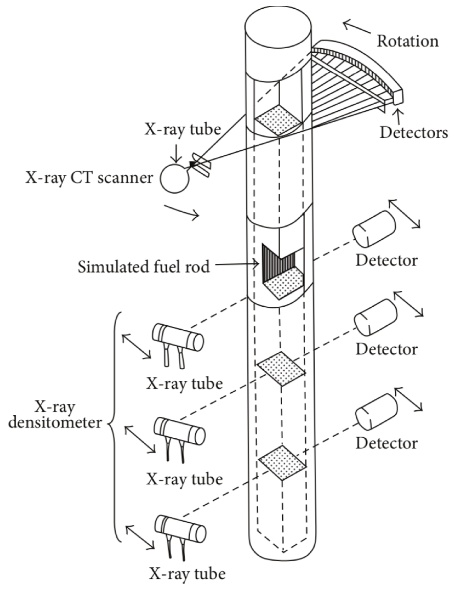
In this research, our primary focus is on utilizing the void fraction (VF) measurements of the BFBT benchmark as our experimental dataset. The experiment facility for the experimental data used in the study is shown in Figure 2. These VF measurements are the key QoIs predicted by the TRACE simulation model. VF data are captured at four distinct locations along the test facility, using X-ray densitometers and X-ray CT scanners. These measurements are designated as ‘Void Fraction 1’ through ‘Void Fraction 4’, corresponding to positions from the lower to the upper regions of the test facility. Experiments with varying boundary conditions (flow rate, inlet temperature, pressure, and power) were conducted and the corresponding VFs were measured. The specifics of the experiments are not in the scope of this study and will not be reiterated here. For further details on the BFBT benchmark, readers can refer to the work in [36].
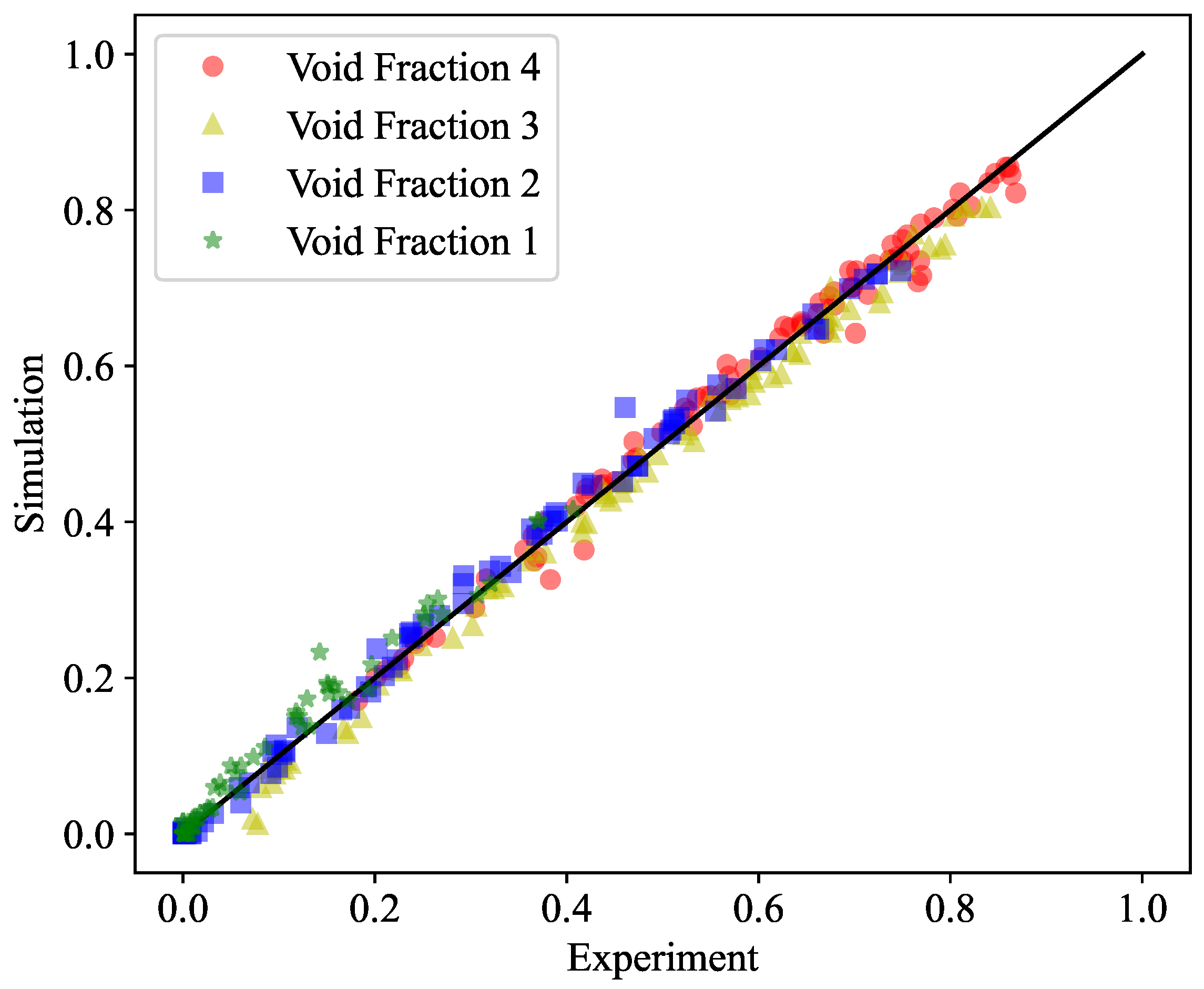
TRACE [56] is a nuclear TH simulation code designed for high-accuracy reactor simulations. In this study, a TRACE model has been developed to align with the experimental geometry and boundary conditions described in the BFBT benchmark. The input parameters of the TRACE model include the geometry specifications and boundary conditions, as well as PMPs. The QoIs are the VF predictions at the corresponding locations. A comparative analysis of the simulated and experimentally measured VF is presented in Figure 3. We can see that the TRACE model predictions exhibit a good agreement with the experimental data, with no major model discrepancy observed.
In this study, we leverage TRACE’s feature that allows the adjustment of 36 PMPs via multiplicative factors. These factors serve as the PMPs in our research. As previously noted, these PMPs are developed for closure laws based on empirical studies, and they may entail significant uncertainties. Consequently, our study aims to quantify the distribution of these PMPs using the BFBT experimental data.

2.3. Hierarchical Bayesian Model

In previous Bayesian calibration settings in the field of nuclear TH, researchers have typically assumed that the observations are mutually independent, allowing the joint likelihood function to be conveniently formulated as the product of each individual likelihood. However, in many situations, especially in nuclear TH codes, such independence may not hold. Wang et al. [32] used a hierarchical Bayesian model to address specific limitations inherent in the single-level Bayesian model, namely the high variability of PMPs under different experimental conditions and the presence of unaccounted-for model discrepancies or outliers, which could lead to overfitting issues. In their study, the hierarchical model is compared with a non-hierarchical model in a TH application and it was demonstrated that the hierarchical model can help make the model more robust against outliers and avoid overfitting. Theoretically, the non-hierarchical model estimates a global variable with equal contributions from each data point, potentially amplifying the outlier impact, while the hierarchical model accommodates calibration parameter variability, thereby offering consistent results given sufficient data. Thus, the hierarchical model has the potential to be applied to larger sets of experimental data. In the current study, we will provide an overview of this hierarchical Bayesian model structure and subsequently extend it to more efficient and scalable applications.
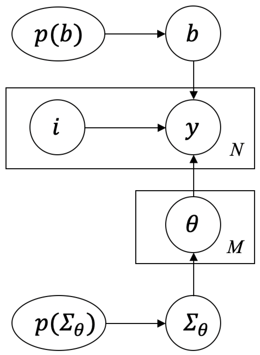
Consider a simple hierarchical model example illustrated in Figure 4. In this graph example, there are N observations  ( y 1 , y 2 , y N ) , shared parameter  b  with prior distribution  p ( b ) , and M group-specific parameter  θ . The shared parameter  b  is assumed to be the same for all observations, while the group-specific parameter  θ  can be different among M groups.  θ  is influenced by its distribution parameters  Σ θ , which have a prior distribution denoted as  p ( Σ θ ) Σ θ  represents the collection of parameters that defines the distributions of  θ , for example, if the M group-specific parameters  θ  are assumed to be from a normal distribution, then  Σ θ  includes two variables: mean and standard deviation. There can be more than one shared parameter so we use a vector  b  to represent the shared parameters in this example.
Figure 4 can also be described as the following generative process:
  • Draw global variables  b p ( b )  and  Σ θ p ( Σ θ ) .
  • Draw group-specific variables  θ i  according to  p ( θ i | Σ θ ) , i = 1 , 2 , M .
  • Draw observed data point  y i p ( y i | θ , b ) , i = 1 , 2 , N .
The joint probability of all the hidden and observed variables, as listed in Figure 4, is
P ( y 1 : N , θ 1 : M , Σ θ , b ) = P ( b ) · P ( Σ θ ) · P ( y 1 : N | θ 1 : M , b ) · P ( θ 1 : M | Σ θ ) .
The posterior distribution of all the variables to be estimated can be described as:
P ( Σ θ , b , θ 1 : M | y 1 : N ) = P ( y 1 : N | θ 1 : M , Σ θ , b ) P ( θ 1 : M , Σ θ , b ) Σ θ , b , θ 1 : M P ( y 1 : N , θ 1 : M , Σ θ , b ) .
In many applications, our main objective is to gain insights about  b  and  Σ θ , rather than the individual group-specific parameters  θ 1 : M . However,  θ 1 : M  also needs to be estimated in order to estimate  Σ θ . Therefore, after acquiring the joint posterior distributions, we must marginalize over the  θ i  parameters.
The likelihood function can be expressed as:
L ( y 1 : N | Σ θ , b ) = θ 1 : M P ( y 1 : N | b , θ 1 : M ) P ( θ 1 : M | Σ θ ) d θ
and the marginalized joint posterior distribution is
P ( Σ θ , b | y 1 : N ) θ 1 : M P ( y 1 : N | b , θ 1 : M ) P ( θ 1 : M | Σ θ ) · P ( b ) P ( Σ θ ) d θ .
This is based on the fact that the prior distribution can be decomposed as  P ( Σ θ , b , θ 1 : M ) = P ( θ 1 : M | Σ θ ) · P ( Σ θ , b )  according to the hierarchical structure.
In many cases, the posterior distribution is in an intractable form, which cannot be analytically solved because of the integral term in the denominator in Equation (5). Therefore, we need to use approximate inference methods to compute the posterior distribution. Two predominant methods for achieving this aim are VI and MCMC. VI generally offers a faster computing speed and focuses on optimizing a well-defined objective, while MCMC has the advantages of being non-parametric and asymptotically exact. In past work within the domain of nuclear TH, MCMC has primarily been employed within the IUQ framework for exploring the posterior distributions. One reason for this preference is that experimental data in nuclear TH are both limited and costly to acquire. Thus, the computational expense of MCMC is justified by its ability to generate highly accurate posterior samples given the limited amount experimental data. However, as hierarchical IUQ frameworks expand to incorporate an increasing number of datasets and applications, which leads to an increasing number of parameters, the need for computational efficiency becomes a crucial consideration.

2.4. Markov Chain Monte Carlo

MCMC methods are based on the idea of generating samples that follow a probability density that is proportional to the posterior distribution without knowing the normalizing constant. The approach is based on the fact that the shape of the posterior distribution remains unaffected by its normalization in Equation (5), eliminating the need for explicit integration during sampling. Many MCMC sampling algorithms have been developed. Early versions of these algorithms employed a strategy of randomly traversing the parameter space using a proposal distribution, creating samples that are either accepted or rejected based on a particular acceptance criterion, thus forming a Markov chain. This process eventually generates a collection of samples approximating the desired distribution. Modern advancements, such as NUTS [57], aim to mitigate issues like random walking and slow convergence attributed to the proposal distribution. As a result, fewer samples are discarded, shorter chains are formed, and faster sampling is achieved. Many MCMC algorithms have been employed in the IUQ framework for the posterior sampling of nuclear TH related applications. For example, the Adaptive Metropolis–Hasting algorithm has been used for the single-level Bayesian model calibration of nuclear TH codes [42], Gibbs sampling has been used in CIRCE methods for similar input UQ applications [4,58]. Recently, the NUTS sampling method was used to sample the posteriors from a hierarchical Bayesian model for the PMPs in nuclear TH simulation codes [32].

2.5. Variational Inference

When a large amount of datasets are available, a hierarchical model typically involves hundreds of parameters to be estimated due to complex hierarchical structures or a large number of groups. VI provides an efficient way to quantify the posterior distributions without sampling the exact posterior distribution. The idea behind VI is to first propose a family of densities and then to find the member of that family that is close to the target [59]. The closeness is measured by Kullback–Leibler (KL) divergence. In this way, VI turns a sampling problem into an optimization problem.
We start with a simple example to illustrate the basic idea of VI. Assume  θ  is the latent variable to be estimated and y is the observation. We can assume them to be scalars without loss of generality. First, we select a family of distributions over the latent variables with its own set of variational parameters  ν , i.e.,  q ( θ | ν ) . Then, we determine the settings of the parameters that make our approximation q as close as possible to the posterior distribution. Afterwards, we can treat q with its fitted parameters to be the posterior.
The KL divergence is a widely used measurement of the closeness of two distributions and the KL divergence between two distributions p and q is defined as:
D KL ( q | | p ) = θ q ( θ ) log q ( θ ) p ( θ | y ) = E q log q ( θ ) p ( θ | y ) .
Now, the inference problem becomes the following optimization problem:
q ( θ ) = argmin q ( θ ) D KL ( q ( θ ) | | p ( θ | y ) ) .
However, this objective function is intractable because it requires the calculation of posterior distribution  p ( θ | y ) , in Equation (8). Instead of directly calculating this objective function, we seek a good approximation. From Equation (8), we can further derive:
D KL ( q ( θ ) | | p ( θ | y ) ) = E log q ( θ ) E log p ( θ , y ) + E log p ( y ) .
Since  log p ( y )  is not dependent on  θ , the expectation value  E log p ( y ) = log p ( y ) . We define the evidence lower bound (ELBO) as:
ELBO ( q ) = E log p ( θ , y ) E log q ( θ ) .
Comparing Equation (10) with Equation (11), we can see that ELBO is the negative KL divergence plus  log p ( y ) , which is a constant with respect to  q ( θ ) . Thus, maximizing ELBO is equivalent to minimizing the KL divergence. If the latent variables are mutually independent and each governed by a distinct factor in the variational density, the joined distributions of  θ 1 : M  can be described as:
q ( θ 1 : M ) = i = 1 M q i ( θ i ) .
Traditionally, it is usually required to develop a custom optimization solution from here, which includes choosing a variational family suited to the model, calculating the relevant objective function, taking derivatives, and running a gradient-based or coordinate-ascent optimization. We can use gradient-based or coordinate ascent inference to iteratively optimize each variational distribution while holding the others fixed. This method is usually referred to as mean field VI. In this paper, we leverage the Automatic Differentiation Variational Inference (ADVI) algorithm [60] implemented in PYMC [61] for inferring the posterior distributions. ADVI offers a recipe for automating the computations involved in VI and provides researchers with a no-manual-tuning method to conduct VI for many models at scale. The general idea of ADVI is to initially transform the inference problem into a common space automatically, and then address the variational optimization. Solving the problem in this common space solves VI for all models in a large class [60].
When comparing VI with MCMC, there are generally two key differences to consider: dataset size and structure of the posterior distribution. VI relies on optimization techniques, so that it can take advantage of methods such as stochastic optimization or distributed optimization. This feature makes VI particularly well-suited for handling large datasets and scenarios that require rapid model exploration. MCMC is better suited for smaller datasets or situations in which one is willing to incur higher computational costs to obtain more precise, theoretically accurate samples. On the other hand, the structure of the posterior distribution is another factor to consider. For many mixture models, Gibbs sampling might be a powerful tool, while for some mixture models, VI may perform better than MCMC even on smaller datasets [62]. Until now, there has been no general conclusion on the relative accuracy of VI and MCMC, and it largely depends on the specific tasks [59]. It should also be noted that the mean field ADVI assumes that the variational posterior distribution is Gaussian without correlation of parameters. In applications where the correlation assumption does not hold, we may use the full-rank Gaussian variational approximation [63] with additional computation cost.

3. Results

3.1. Synthetic Data Example

3.1.1. Problem Definition

The synthetic data example is designed to mirror the application of the system TH code with BFBT void fraction data, which we will explore in later sections. Suppose we have three parameters to estimate  [ θ 1 , θ 2 , θ 3 ] , and we know that observations  y  are from a quadratic function ( X  is determined):
y = θ 1 X 2 + θ 2 X + θ 3 I + N ( 0 , σ e 2 ) .
In real-world applications, we can consider  [ θ 1 , θ 2 , θ 3 ]  to be the PMPs, and the quadratic function to be a more complex simulation models. Our goal now is to estimate the posterior distribution of  [ θ 1 , θ 2 , θ 3 ]  given the function form, experimental observations  y , and control variables  X . We generate  N = 300  groups of data and let each group contain  M = 6  data points. The true values of  [ θ 1 , θ 2 , θ 3 ]  have slight variability among different groups, and they are generated from the normal distributions defined below:
θ 1 N ( 10 , 3 ) θ 2 N ( 2 , 1.5 ) θ 3 N ( 5 , 2 ) .
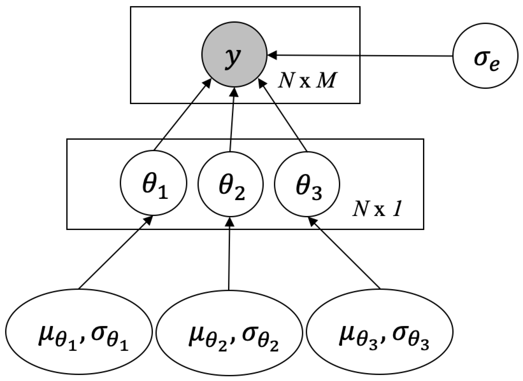
To account for the variation in latent parameters  [ θ 1 , θ 2 , θ 3 ]  among different groups, a Bayesian hierarchical model is utilized to tackle this concern. Since we know that they are generated from normal distributions, we can define their corresponding hyper-parameters using mean and standard deviation of the normal distribution:  μ θ 1 , σ θ 1 , μ θ 2 , σ θ 2 , μ θ 3 , σ θ 3 . A visual representation of the model structure is presented in Figure 5.

3.1.2. Results and Discussions

Following the hierarchical structure defined above, the generative process is as follows:
  • Draw samples of global variables, ( μ θ 1 , σ θ 1 , μ θ 2 , σ θ 2 , μ θ 3 , σ θ 3 ), from their prior distributions. We use wide uniform distributions as priors to reflect our ignorance of knowledge.
  • For  i = 1 , 2 , 3  and  n = 1 , 2 , N , draw samples of group-specific parameters  θ i n N ( μ θ i , σ θ i ) .
In this structure, Bayesian inference needs to estimate an extensive set of  307 ( 300 + 6 + 1 = 307 )  parameters. Traditional random sampling-based MCMC algorithms are impractical for managing this level of complexity. There are more advanced algorithms to deal with this situation. While Gibbs sampling could offer a solution, as it is relatively easy to derive all the conditional distributions in this context, this approach may not be feasible for more complex problems or for scalability across multiple models or datasets because it requires us to analytically derive all the conditional distributions for each problem, making it hard to scale. There are several advanced algorithms that require minimal hand-tuning for conducting Bayesian inference, making them suited for large-scale applications. In this work, we use two such algorithms that require minimal hand-tuning—NUTS and ADVI. They are both implemented in the PYMC [61] package and can be easily integrated with other applications.
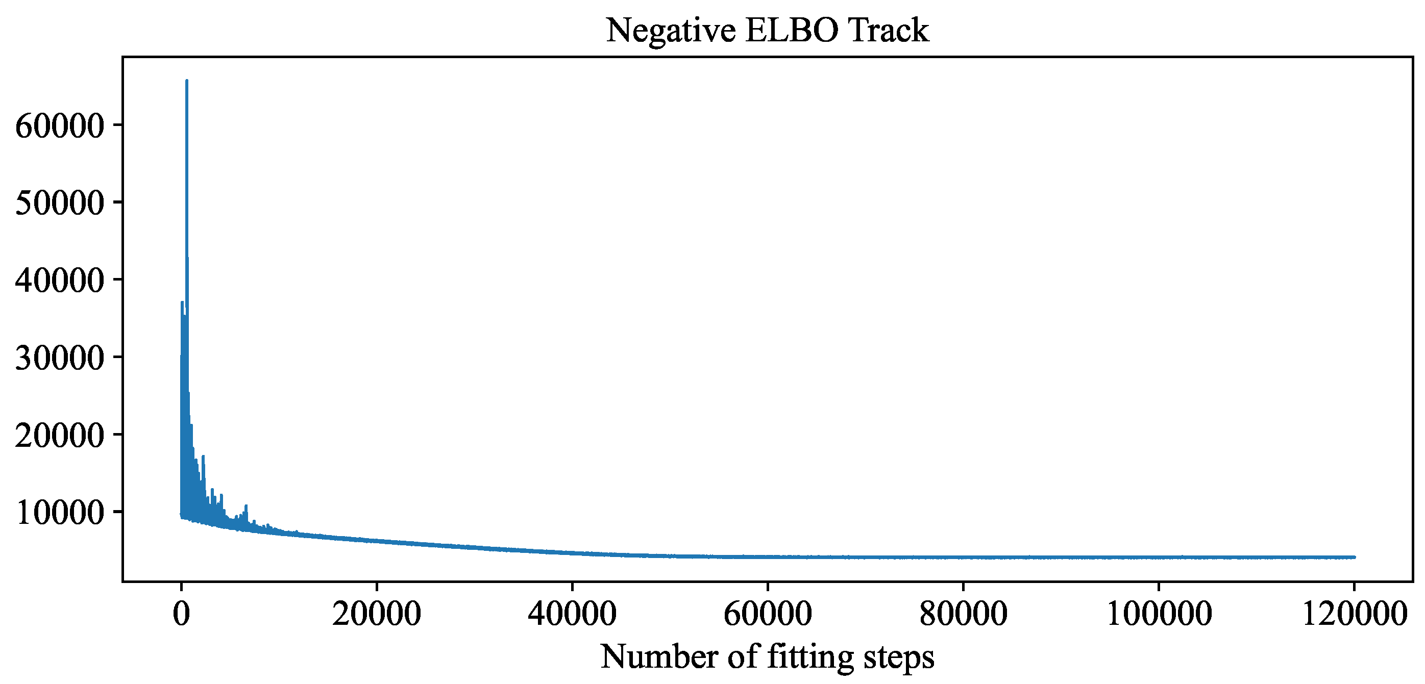
For the NUTS sampler, we draw 6000 samples in total and use the first 1000 as tuning samples. The number of samples is based on the convergence of the MCMC chain, which can be confirmed by the mixture of trace plot and by checking if multiple parallel runs yield the same result. For ADVI, we can track the ELBO during the optimization steps to see if the algorithm has converged. In ADVI, the loss function is the negative of ELBO and it is plotted in Figure 6. We can see it is converged after 100,000 steps. It should be noted that the negative ELBO in ADVI is not normalized so the absolute value cannot be compared across models.
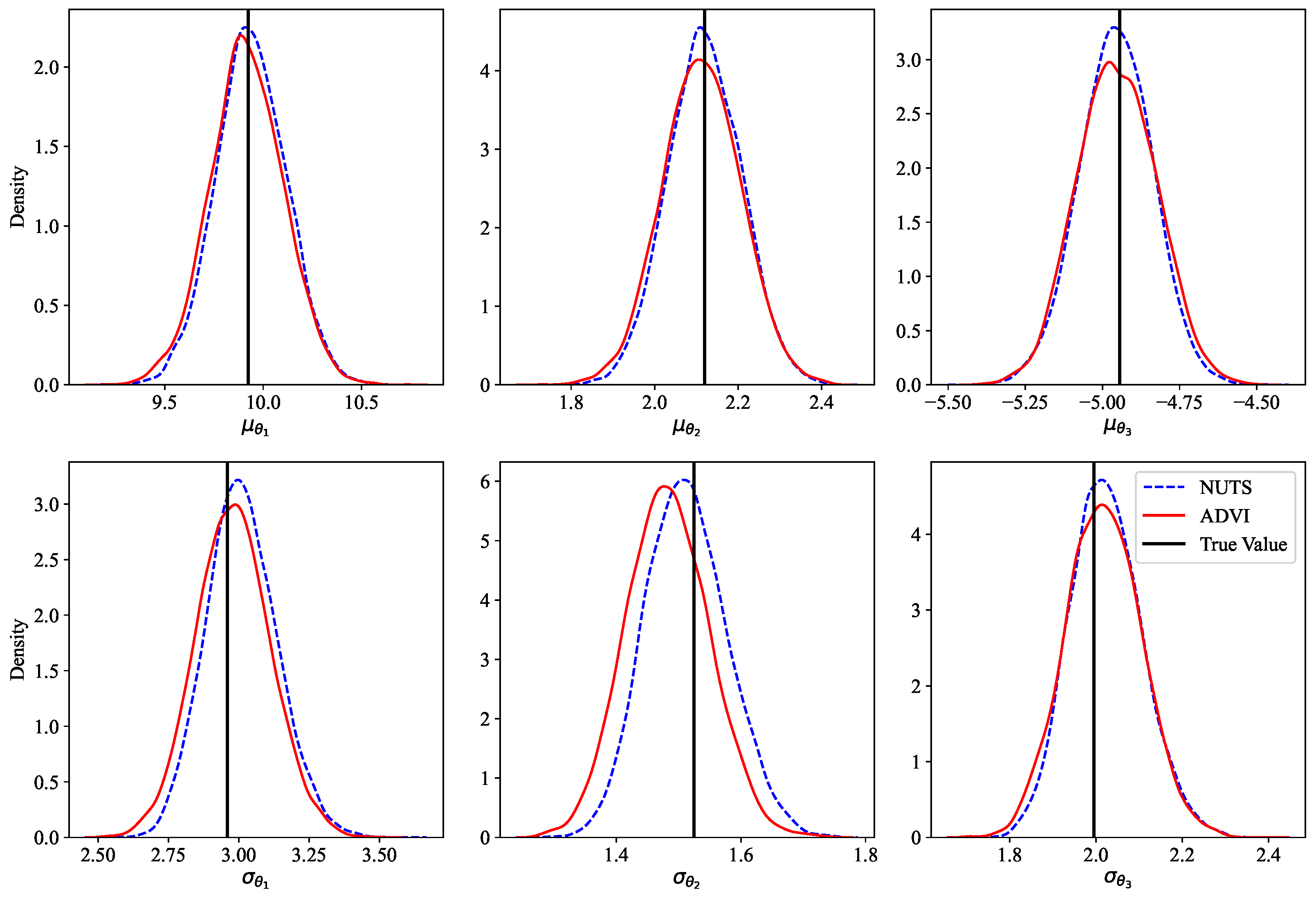
After the posterior samples are obtained from both algorithms, we can compare their posterior distributions. We are mainly interested in the hyper-parameters ( μ θ 1 σ θ 1 μ θ 2 σ θ 2 μ θ 3 σ θ 3 ) and their posteriors are displayed in the Kernel Density Estimate (KDE) plot in Figure 7. From the results we can see that both algorithms are capable of accurately estimating the true values of the parameters in this example. In many real-world applications, the true values are not known, so we need to conduct further PPC to confirm the obtained distributions, but it is not necessary in this synthetic data example.
Computing time is another important factor to compare. As summarized in Table 1, ADVI demonstrates a significant speed advantage by accomplishing 120,000 fitting steps in 12 s. In contrast, the NUTS algorithm requires more time and it takes 50 s to generate 6000 samples. The computations were performed on an identical hardware configuration, specifically on a single core of an Apple M1 Pro chip, utilizing the software package PYMC 5.9.2. It should be noted that both steps here correspond to the total number of calls to the computation model. In this toy example, it is the quadratic function. In the TH application later, this correspond to the number of calls to the surrogate model. Theoretically, ADVI offers an additional layer of scalability due to its amenability to parallelization—owing to its nature as an optimization algorithm. Conversely, the NUTS algorithm inherently requires sequential generation, which restricts its parallelization capabilities. Furthermore, ADVI can further utilize mini-batch optimization techniques to expedite computations, particularly when dealing with extensive datasets including tens of thousands of data points. This offers a potentially advantage in scenarios demanding rapid scaling to large datasets.

3.2. Nuclear Thermal-Hydraulics Application

3.2.1. Problem Definition

In Section 2.2, we have introduced the background for the BFBT benchmark and the TRACE simulation model. In this study, we will use the PMPs in TRACE as uncertain inputs, and our primary goal is to estimate the posterior distribution of the PMPs given the experimental data in BFBT benchmark, as derived in Equation (2). In TRACE, a total of 36 PMPs, including variables like liquid-to-interface transition heat transfer coefficients, wall drag coefficients, and interfacial drag coefficients, are available for adjustment. However, not all of these parameters are necessarily pertinent to the current modeling task, thus a sensitivity analysis is used to screen out non-important parameters. This can significantly reduce the number of parameters in the subsequent studies and thus reduce the computational cost. Four parameters are selected out of thirty-six, given their dominant impacts on the model QoIs, and they are listed in Table 2. More details on the parameter selection procedure will be given in the following section.
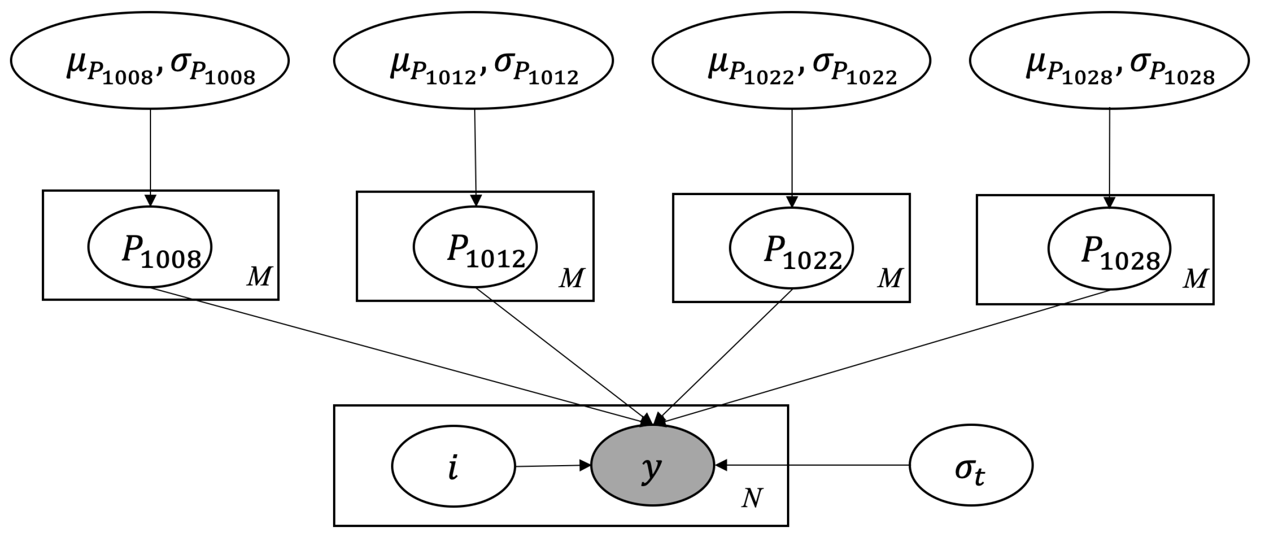
The dataset used for IUQ consists of 86 experimental groups. Each group represents a set of steady-state measurements obtained from the test facility and includes four VF measurements at different elevations of the test assembly. Given that these experimental groups were conducted under varying boundary conditions (e.g., heat flux, temperature, pressure), it is reasonable to hypothesize that PMPs within the same group exhibit similar behavior, while they may diverge under different conditions. Accordingly, a hierarchical Bayesian framework is employed to model this structure, as shown in Figure 8.
The PMPs (denoted as  P 1008 P 1012 P 1022 P 1028 ) could be different among  M = 86  groups, so we assume each of them is from a common normal distribution governed by its hyper-parameters (i.e., the mean and standard deviation of the normal distribution). For example, for  P 1008 :
P 1008 N ( μ P 1008 , σ P 1008 2 ) .
This approach accommodates variations of PMP from one experiment to another, which can be caused by potential errors, discrepancies, or different physical conditions. Some experimental data may have relatively large discrepancy due to unknown or unaccounted factors, and they may have more significant influence on the likelihood function than other “good” data points, thus making the posterior distribution results sensitive to them. These data points may also be considered as “outliers”. By using this hierarchical framework, we can concentrate on modeling the distribution of PMPs in a way that makes it robust to outliers. If proper prior information is added to  μ  and  σ , we can conduct Bayesian inference and obtain their posterior distribution.
We employ wide uniform priors for the selected parameters to reflect our limited prior knowledge. To ensure the robustness of our posterior estimates, an iterative re-sampling methodology is utilized, as elaborated in previous works [32,33]. This procedure verifies that the specified prior range is sufficiently broad to encompass the posterior distribution, mitigating the influence of prior range selection on posterior outcomes. The priors of all the hyper-parameters, following Figure 8, are shown in Table 3.
Additionally, we introduce  σ t , defined in Equation (3), as a term representing the total variance. Given the lack of explicit knowledge about all the components that contribute to this term,  σ t  is treated as an uncertain input parameter that requires estimation. In cases where all the components of  σ t  are known, such as when GP is used as the surrogate model and code uncertainty becomes available, we may directly incorporate it without the need for further estimation.

3.2.2. Sensitivity Analysis and Surrogate Model

Having gathered all the requisite elements to execute Bayesian inference for estimating the posterior distribution as described in Equation (2), there remain several obstacles specific to nuclear TH applications within the IUQ framework. One such challenge is the potentially high number of input parameters. As previously discussed, it is crucial to employ SA methods to identify the most influential parameters, thereby streamlining subsequent computational efforts. Another impediment lies in the computational intensity of the TRACE simulation code. Each TRACE simulation may require several minutes or more to complete. Given that Bayesian inference necessitates tens of thousands of samples, the direct utilization of TRACE becomes infeasible due to the excessive computation time. Additionally, VI calls for derivatives of the model output with respect to the input; this is also a new requirement that TRACE cannot readily fulfill. To circumvent this issue, we employ machine learning-based regression models to serve as surrogate models for the TRACE code. In this section, we will briefly introduce the SA methods and surrogate models used in this work.
In the initial stage of parameter selection, a simple perturbation approach is deployed. Each parameter is individually perturbed within the range of  ( 0 , 5 ) , while all other parameters remain fixed. We employ 50 uniform samples within this range to evaluate the impact of each parameter on the simulated void fraction data. The output variance attributable to each parameter is then computed. Our findings reveal that the majority of the variances are either zero or negligibly close to it. From this preliminary examination, eight parameters boasting variances greater than  10 3  are singled out for further investigation.
However, the quantitative impact of these parameters on the QoIs varies significantly. Carrying out Bayesian inference on all these parameters could lead to computational redundancy. To address this, the Sobol indices method is subsequently invoked for a more detailed screening. The Sobol indices method provides a straightforward measure of sensitivity in arbitrarily complex computational models [64]. Essentially, it is a variance-based approach that decomposes the output variance into individual and interactive contributions from each input variable, a technique known as ANOVA (ANalysis Of VAriance). For the computation of Sobol indices, we adhere to the sampling-based strategy outlined by Saltelli et al. [64] and utilize the Sensitivity Analysis Library in Python [65]. Given its widespread successful application in various UQ contexts [45,55,66] in the field, the specifics of the Sobol indices will not be reiterated here. As a result of this refined screening process, a subset of four parameters emerges as having a dominant influence on the model’s QoIs. These are therefore selected as the uncertain inputs for subsequent analyses in the IUQ framework.
Given the inputs and the model QoIs, we can build a regression model that will serve as a surrogate for the computationally intensive TRACE simulation code. The surrogate model aims to accurately approximate the TRACE simulations on the given input–output domain, while significantly reducing the computational cost. For the surrogate model, techniques such as polynomial chaos expansions, polynomial regression, Gaussian processes, and neural networks are commonly employed, depending on the specific nature of the task. These techniques are trained on a dataset generated from a carefully designed set of TRACE simulations to ensure that the surrogate model captures the input–output relationships inherent in the original TRACE model. The trained surrogate model is then validated using separate sets of data to confirm its predictive accuracy. Once validated, the surrogate model can be integrated into the Bayesian inference framework, thereby enabling efficient and scalable IUQ analyses.
In this work, we employ a polynomial regression (PR) model because it was discovered that the output void fractions exhibit a relatively simple relation to the input PMPs in the prior ranges. The PR model with a degree of d for two variables  x 1 , x 2  has the following form:
y ^ ( w , x ) = w 0 + w 1 x 1 + w 2 x 2 + w 3 x 1 x 2 + w 4 x 1 2 + w 5 x 2 2 + + w n x 1 d + w n + 1 x 2 d .
Another major reason for employing the PR-based surrogate model is due to its compatibility with the NUTS sampling algorithm, which requires gradient information. As a parametric regression model, it is relatively straightforward to compute the gradient at any specified location. While GPs and neural networks could also be appropriate choices for surrogate modeling for NUTS sampling, the PR model offers a balance between sufficient accuracy and computational simplicity for our current problem setting.
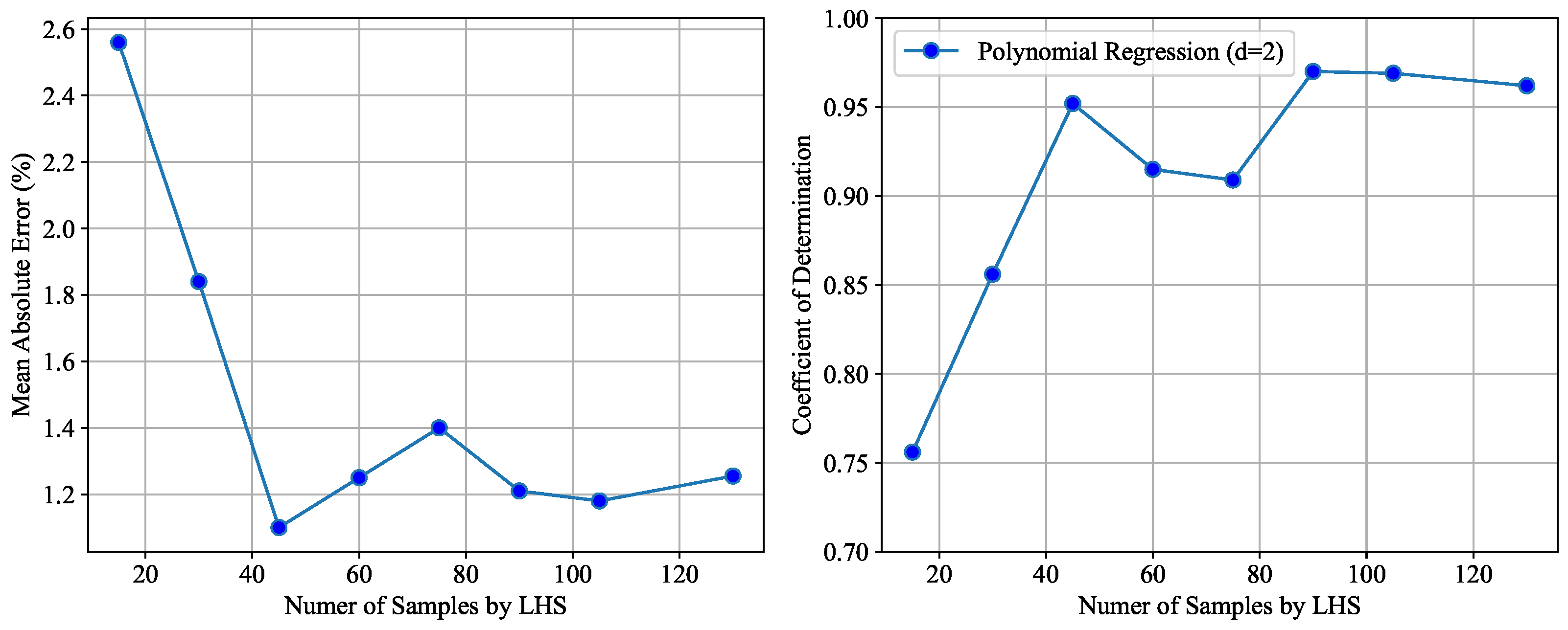
To validate the performance and suitability of the PR model, we conduct a convergence study focusing on the accuracy of the surrogate model on a separate validation dataset. This study can help determine the minimum number of samples required to construct an accurate surrogate model. Latin Hypercube Sampling (LHS) is used to sample from the input domain. The Mean Absolute Error (MAE) and Coefficient of determination ( R 2 ) on an additional 25 validation data points is shown in Figure 9. The graph indicates that the out-of-sample error rates stabilize when the sample count exceeds 100. The observed MAE falls within a range of 1% to 1.25%, which is deemed acceptable for the present study. This is because the reported experimental measurement error for the void fraction is absolute 3%; thus, a relative error of 1% is well below this value. Additionally, the  R 2  indicates that the surrogate models offer a reliable approximation of the original TRACE simulation code when the sample size surpasses 100. As a result, we used 100 LHS samples to construct our surrogate models for subsequent studies.

3.2.3. Results

Now that we have constructed accurate surrogate models, we can use the hierarchical structure defined in Figure 8 to infer the posterior distributions. We apply both NUTS and ADVI methods and compare the generated posterior distributions as well as the computing efficiency. For the NUTS algorithm, a total of 100,000 samples were generated, with the initial 20,000 serving as tuning samples and excluded from the final posterior samples. Convergence of the Markov chains was assessed through the inspection of trace plots and by confirming that multiple parallel runs yielded consistent outcomes. In the case of ADVI, we performed 300,000 fitting steps, and convergence was confirmed by tracking the ELBO. The negative ELBO track for this application closely resembles that presented in Figure 6 and, therefore, will not be repeated here.
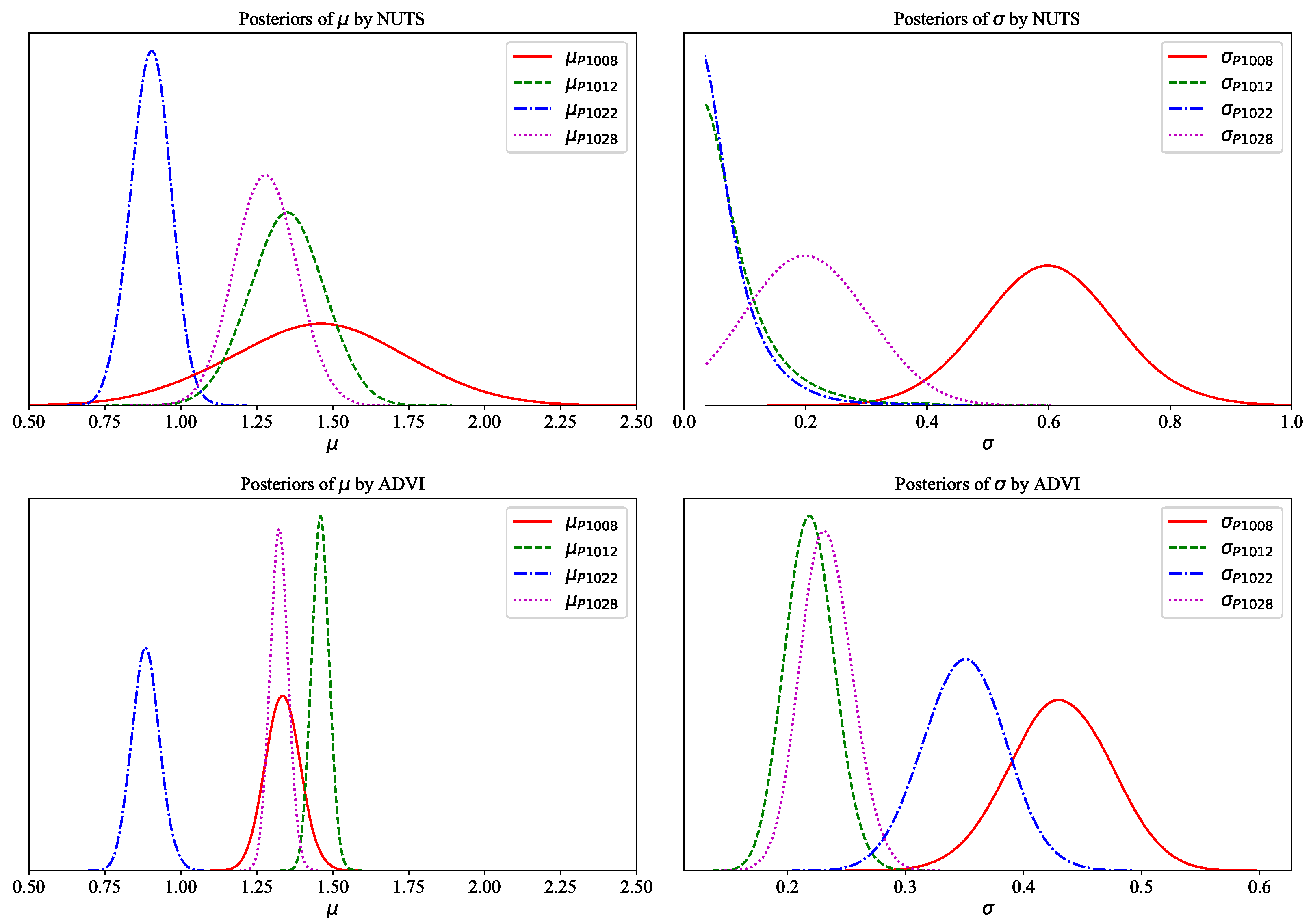
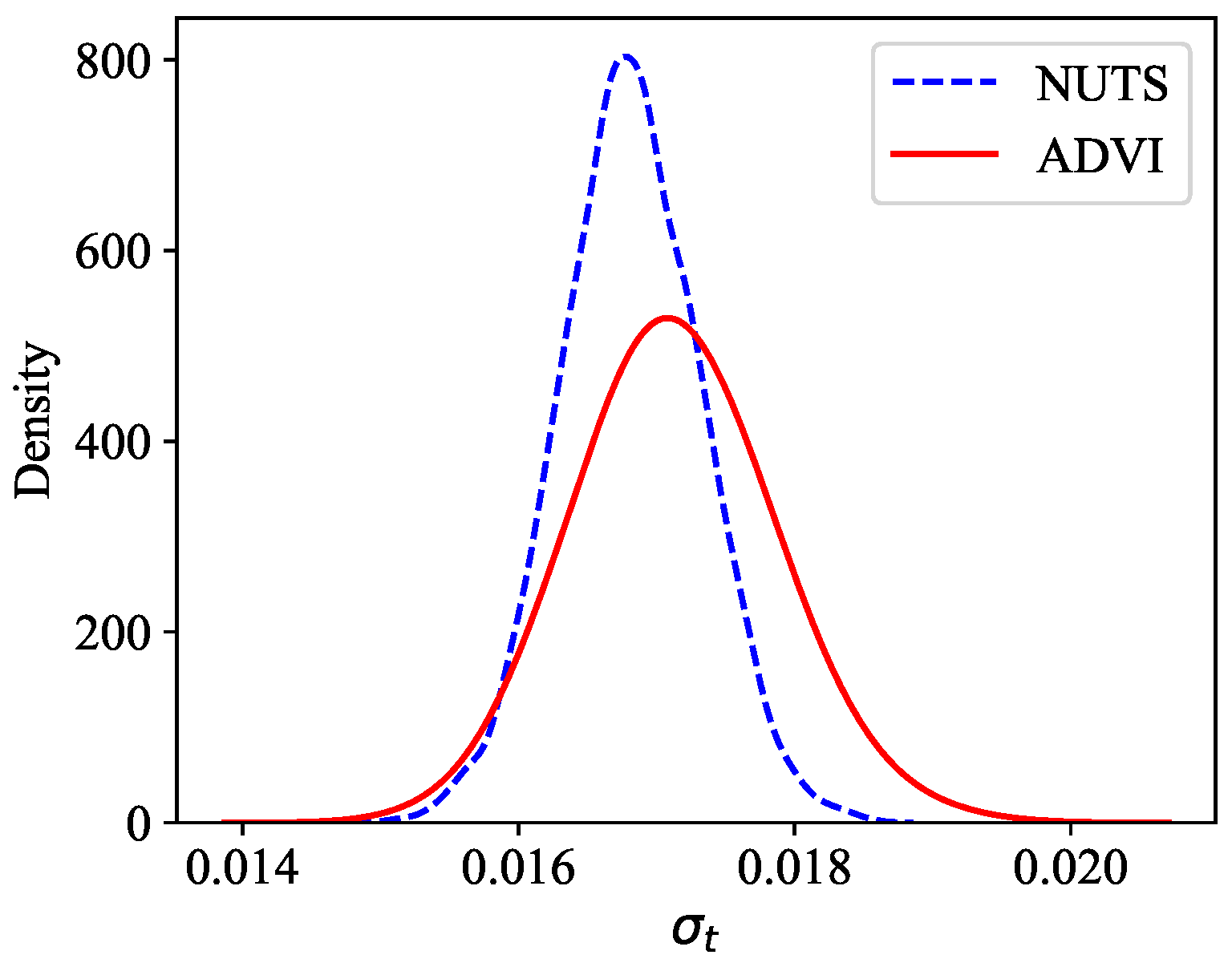
Figure 10 shows the posteriors of hyper-parameters ( μ P 1008 σ P 1008 μ P 1012 σ P 1012 μ P 1022 σ P 1022 μ P 1028 σ P 1028 ) generated by KDE plots. These are the mean values and standard deviations of the normal distributions that generate the PMPs. While both methods yield similar results for certain parameters, noticeable discrepancies exist for some others. Specifically, the posteriors for  P 1008  and  P 1028  ( μ P 1008 μ P 1028 σ P 1008 σ P 1028 ) show similar modes, but ADVI generates a smaller variance of the posterior distributions. For parameters  P 1012  and  P 1022 , their standard deviation posteriors ( σ P 1012 σ P 1022 ) are vastly different, and their mean posteriors ( μ P 1012 μ P 1022 ) are generally similar, but  P 1022  shows slightly more divergence. The total variance term  σ t  has a relatively better agreement between the two approaches, as shown in Figure 11.
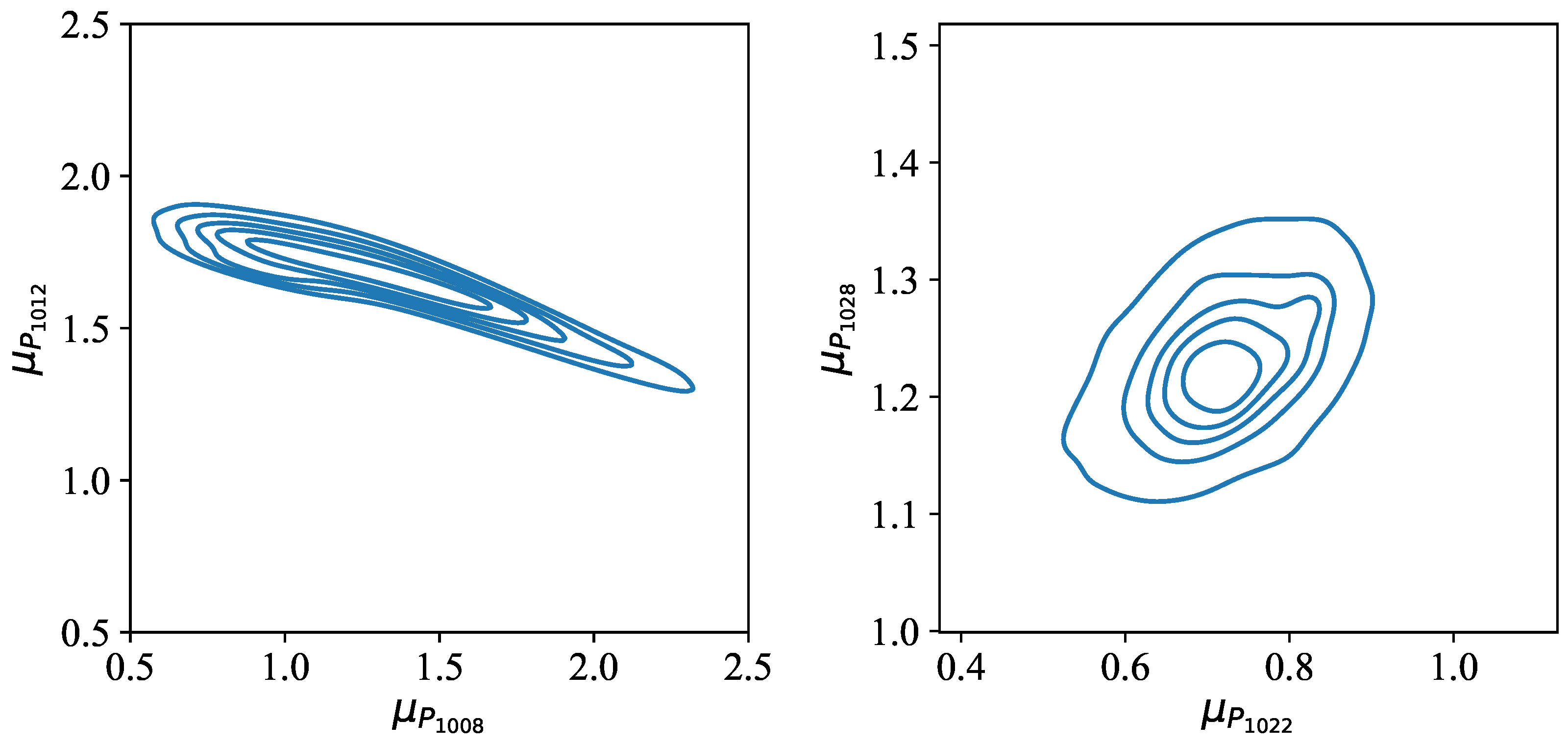
One critical difference between the NUTS and ADVI methods lies in their treatment of variable correlations. ADVI employs mean field VI, which assumes independence between all the variables and uses Gaussian distribution as the variational approximations. Thus, its posteriors always look Gaussian. NUTS, in contrast, accounts for the correlations among latent parameters during the sampling stage. Using the NUTS algorithm, we observed correlations between the pairs ( μ P 1008 μ P 1012 ) and ( μ P 1022 μ P 1028 ), and their correlations can be visualized in Figure 12 using bivariate KDE plots. Previous studies also affirm these correlations among the PMPs in TRACE, which can be rationalized based on their physical meanings [41]. For example,  P 1008  is the single phase liquid to the wall heat transfer coefficient and  P 1012  is the subcooled boiling heat transfer coefficient; they both positively influence the QoI (void fraction) as the heat transfer coefficient increases. It should be noted that the full-rank ADVI method can account for correlations among variables by using a multivariate Gaussian distribution as the variational approximation. However, it comes at a computational cost and can be prohibitively slow for large data [62]. Comparing and evaluating full-rank ADVI in IUQ applications can be an interesting direction for future research.
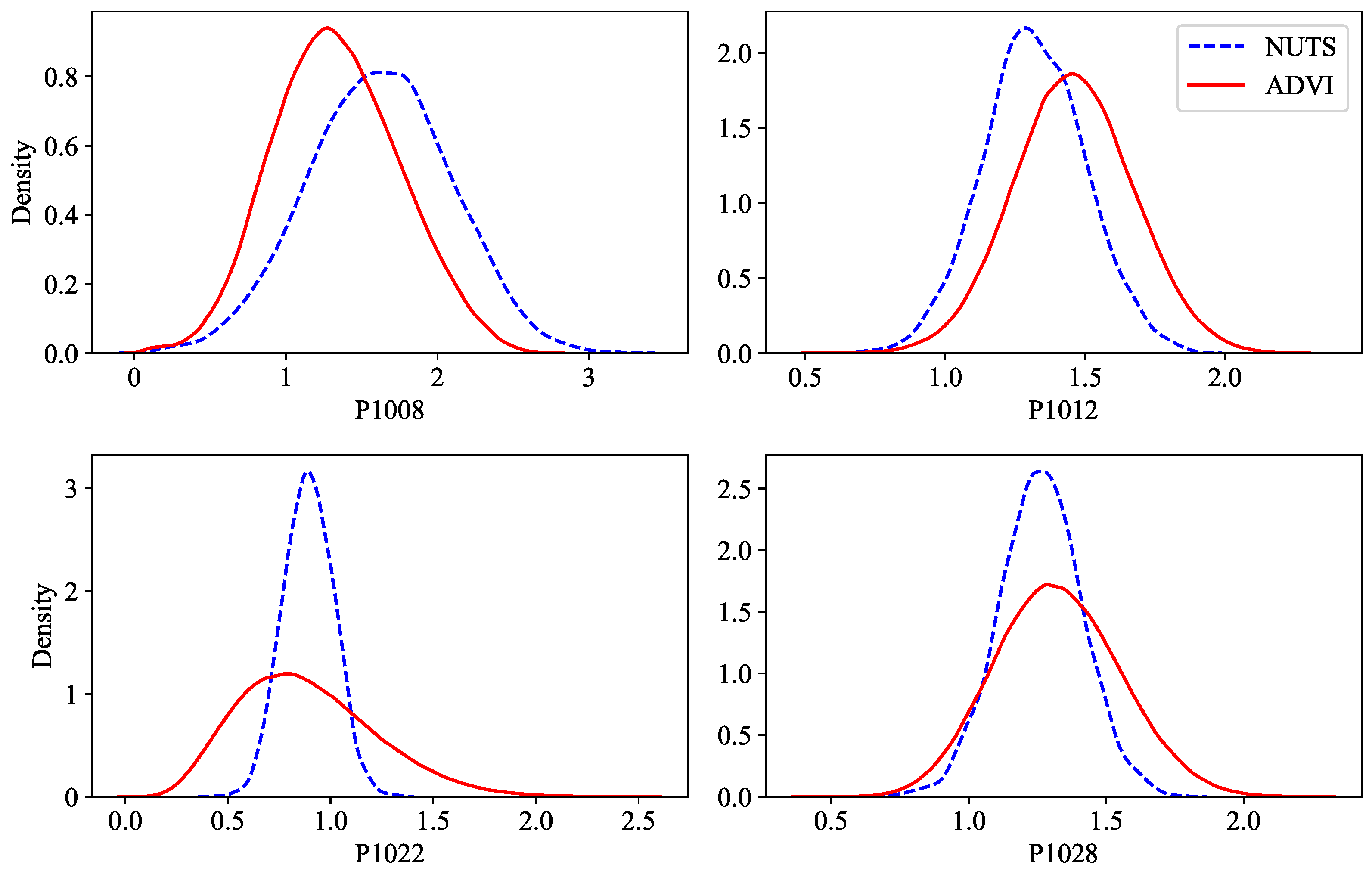
Due to the difference in dealing with correlations, the results obtained by ADVI and NUTS show divergent behaviors on certain parameters. However, in the IUQ framework, our primary focus is on the distributions of the PMPs rather than their hyper-parameters, because these PMP distributions are essential for FUQ analysis. To this end, posterior samples of PMPs are generated using their corresponding hyper-parameter posterior samples. Figure 13 compares these posteriors and reveals generally similar behaviors for the PMPs from both NUTS and ADVI methods. Some differences are noted, particularly for the parameter  P 1022 , but the results align well overall. The posteriors of the PMPs are fitted using normal distribution and are summarized in Table 4.
While it is generally challenging to justify one set of results as “better” without knowing the true values, we can use PPC as a confirmation strategy. PPC provides the comparison between the updated model (using the posteriors of PMPs) and the original model (using the default PMP values), against the observed data. From this process we can see whether the updated model performs better than the original model, in terms of reducing the discrepancy between the model predictions and experimental observations.
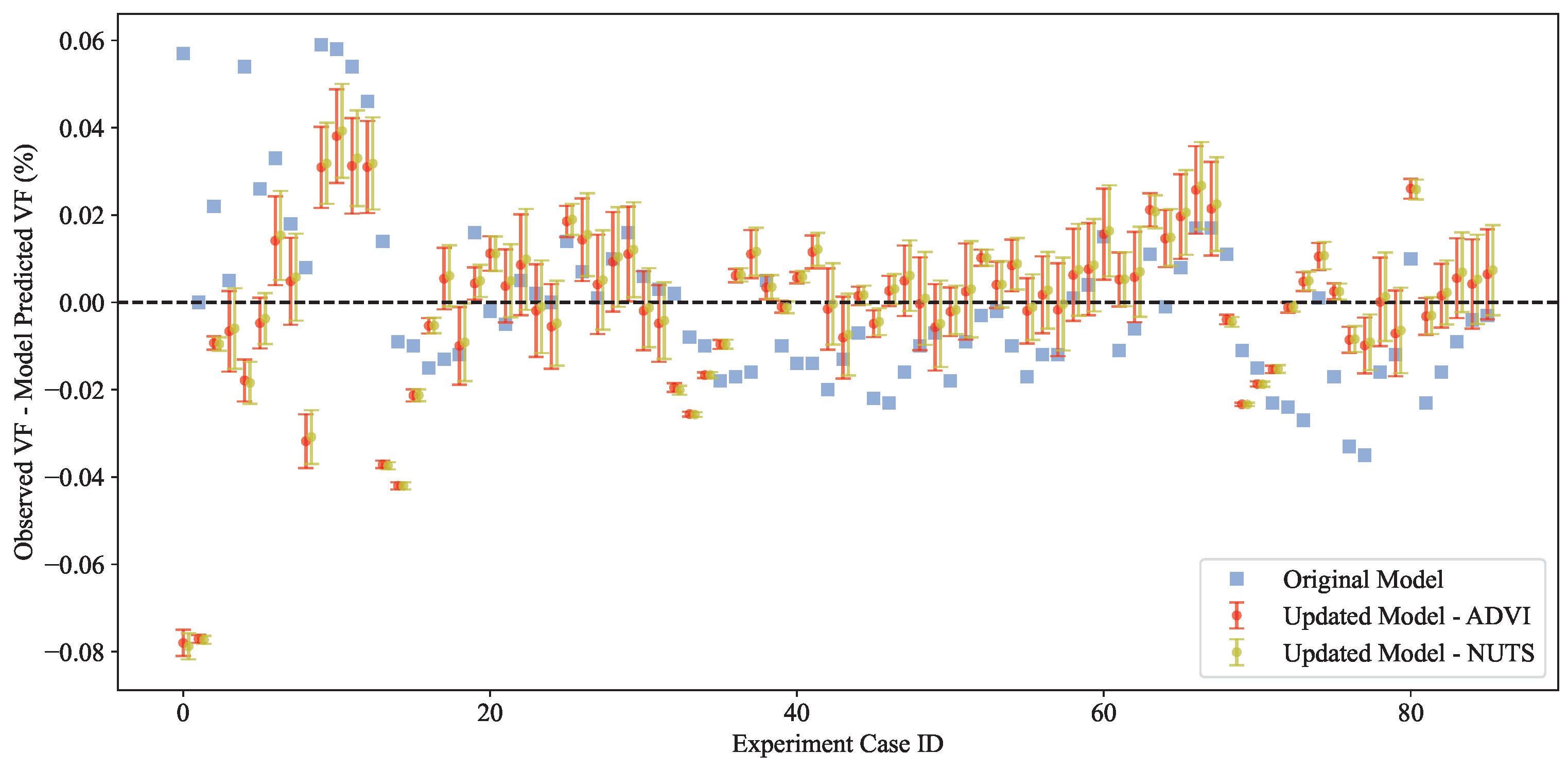
We can conduct the PPC and FUQ in the same step. We firstly generate 1000 samples from the posteriors reported in Table 4 and use them as the input of the simulation models. We can then compute the simulation results and summarize their means and standard deviations. The results for void fraction measurement location 4 is presented in Figure 14. The figure includes 86 experimental cases, indexed on the x-axis from 0 to 85. The y-axis shows the observed VF minus the predicted VF, indicating the discrepancy between the experimental data and the simulation model.
From this analysis, we can draw two main conclusions. First, the updated models using different algorithms yield very similar predictions, even though slightly different posterior distributions via the ADVI and NUTS methods are obtained. This concordance could potentially be attributed to underlying interactions between parameters, and NUTS and ADVI treat them differently. Second, the updated models exhibit lesser discrepancies compared to the original TRACE model, indicating that the Bayesian IUQ has improved the agreement between model/data. The 2.5–97.5 percentiles do not provide sufficient empirical coverage for the simulation data; this is partially due to the existence of other types of uncertainty, such as boundary conditions and geometry. The FUQ results here only account for the parametric uncertainty caused by the selected PMPs. For the sake of brevity, results for the other three measurement locations are not presented here since they yield similar conclusions.
Finally, we compare the computing efficiency between the two inference algorithms. Similar to the synthetic data example, Table 5 shows the computing times associated with the two algorithms. ADVI shows significant faster computing speed and is able to achieve converged results within 1 min, while it takes about 23 min for NUTS algorithm to achieve a converged MCMC chain. This efficiency gain positions ADVI as an attractive option for similar IUQ studies, particularly when computational resources are constrained or when we want to quickly extend the framework to multiple datasets and applications.

4. Conclusions and Future Work

In this study, we have developed and demonstrated an extension to the existing Bayesian IUQ framework that employs a hierarchical Bayesian model and VI to quantify uncertainties of PMPs more efficiently than most of the previous studies using MCMC sampling. The proposed approach offers a scalable, efficient, and accurate means to obtain the posteriors of PMPs. We provided a comprehensive comparison between the proposed method and a hierarchical model that utilizes NUTS sampling in a previous study [32]. Through a synthetic data experiment and a case study on IUQ of TRACE based on the BFBT benchmark data, we demonstrated that our VI-based method delivers significant computational advantages without sacrificing the quality of the posterior estimates. Similarly to the NUTS algorithm, the VI-based method requires no manual tuning, thereby extending its utility across diverse applications with minimal adjustments.
We note that, while VI and NUTS generated different posterior distributions for certain hyper-parameters, their predictive performance, as determined by PPC and FUQ, showed similar results. This suggests that the hierarchical Bayesian IUQ framework is robust to the choice of the inference algorithms. The difference could be attributed to the correlations between the parameters, because ADVI assumes that all parameters are independent during the optimization process. This can potentially limit the applicability of ADVI in scenarios where capturing such correlations is desired. But in applications where we are mainly interested in the final distributions of PMPs, such simplification is acceptable. The correlations also lead to the “identifiability” issue in IUQ, which remains an active research area.
For future research, the framework can be extended to incorporate more sophisticated surrogate models for more complex problems, such as those with strong non-linearity. Additionally, the currently example does not consider model discrepancy, while model discrepancy can play an important role in IUQ [1]. Exploring the potential benefits of the hierarchical model when model discrepancy exists can also be an interesting area.

Author Contributions

Conceptualization: C.W., X.W., Z.X. and T.K.; methodology: C.W. and X.W.; software: C.W.; validation: C.W., X.W. and Z.X.; writing—original draft preparation: C.W.; writing—review and editing: C.W., X.W., Z.X. and T.K. All authors have read and agreed to the published version of the manuscript.

Funding

This research received no external funding.

Data Availability Statement

No new data were created or analyzed in this study. Data sharing is not applicable to this article.

Conflicts of Interest

The authors declare no conflict of interest.

Abbreviations

The following abbreviations are used in this manuscript:
ADVIAutomatic Differentiation Variational Inference
BFBTBWR Full-size Fine-mesh Bundle Test
ELBOEvidence Lower Bound
FUQForward Uncertainty Quantification
GPGaussian Process
IETIntegral-effect test
IUQInverse Uncertainty Quantification
KDEKernel Density Estimate
LHSLatin Hypercube Sampling
MAEMean Absolute Error
MCMCMarkov Chain Monte Carlo
NUTSNo-U-Turn-Sampler
PMPPhysical Model Parameters
PPCPosterior Predictive Check
PRPolynomial Regression
QoIQuantity-of-Interest
SETSeparate-Effect Test
THThermal-Hydraulics
UQUncertainty Quantification
VBMCVariational Bayesian Monte Carlo
VFVoid Fraction
VIVariational Inference
VVUQVerification, Validation, and Uncertainty Quantification

References

  1. Wu, X.; Xie, Z.; Alsafadi, F.; Kozlowski, T. A comprehensive survey of inverse uncertainty quantification of physical model parameters in nuclear system thermal–hydraulics codes. Nucl. Eng. Des. 2021, 384, 111460. [Google Scholar] [CrossRef]
  2. Kennedy, M.C.; O’Hagan, A. Bayesian calibration of computer models. J. R. Stat. Soc. Ser. B Statistical Methodol. 2001, 63, 425–464. [Google Scholar] [CrossRef]
  3. Bui, A.; Williams, B.; Dinh, N. Advanced Calibration and Validation of a Mechanistic Model of Subcooled Boiling Two-Phase Flow. In Proceedings of the International Congress on Advances in Nuclear Power Plants, Charlotte, NC, USA, 6–9 April 2014. [Google Scholar]
  4. Damblin, G.; Gaillard, P. Bayesian inference and non-linear extensions of the CIRCE method for quantifying the uncertainty of closure relationships integrated into thermal-hydraulic system codes. Nucl. Eng. Des. 2020, 359, 110391. [Google Scholar] [CrossRef]
  5. Skorek, T.; de Crécy, A.; Kovtonyuk, A.; Petruzzi, A.; Mendizábal, R.; de Alfonso, E.; Reventós, F.; Freixa, J.; Sarrette, C.; Kyncl, M.; et al. Quantification of the uncertainty of the physical models in the system thermal-hydraulic codes–PREMIUM benchmark. Nucl. Eng. Des. 2019, 354, 110199. [Google Scholar] [CrossRef]
  6. Baccou, J.; Zhang, J.; Fillion, P.; Damblin, G.; Petruzzi, A.; Mendizábal, R.; Reventós, F.; Skorek, T.; Couplet, M.; Iooss, B.; et al. SAPIUM: A Generic Framework for a Practical and Transparent Quantification of Thermal-Hydraulic Code Model Input Uncertainty. Nucl. Sci. Eng. 2020, 194, 721–736. [Google Scholar] [CrossRef]
  7. Ghione, A.; Sargentini, L.; Damblin, G.; Fillion, P.; Baccou, J.; Sueur, R.; Iooss, B.; Petruzzi, A.; Zeng, K.; Zhang, J.; et al. Applying the SAPIUM guideline for Input Uncertainty Quantification: The ATRIUM project. In Proceedings of the 20th International Topical Meeting on Nuclear Reactor Thermal Hydraulics (NURETH-20), Washington, DC, USA, 20–25 August 2023. [Google Scholar]
  8. Liu, Y.; Hu, R.; Zou, L.; Nunez, D. SAM-ML: Integrating data-driven closure with nuclear system code SAM for improved modeling capability. Nucl. Eng. Des. 2022, 400, 112059. [Google Scholar] [CrossRef]
  9. Damblin, G.; Bachoc, F.; Gazzo, S.; Sargentini, L.; Ghione, A. A generalization of the CIRCE method for quantifying input model uncertainty in presence of several groups of experiments. arXiv 2023, arXiv:2306.02762. [Google Scholar] [CrossRef]
  10. Xie, Z.; Alsafadi, F.; Wu, X. Towards improving the predictive capability of computer simulations by integrating inverse Uncertainty Quantification and quantitative validation with Bayesian hypothesis testing. Nucl. Eng. Des. 2021, 383, 111423. [Google Scholar] [CrossRef]
  11. Helleckes, L.M.; Osthege, M.; Wiechert, W.; von Lieres, E.; Oldiges, M. Bayesian calibration, process modeling and uncertainty quantification in biotechnology. PLoS Comput. Biol. 2022, 18, e1009223. [Google Scholar] [CrossRef]
  12. Mosser, L.; Zabihi Naeini, E. A comprehensive study of calibration and uncertainty quantification for Bayesian convolutional neural networks—An application to seismic data. Geophysics 2022, 87, IM157–IM176. [Google Scholar] [CrossRef]
  13. Ye, J.; Mahmoudi, M.; Karayagiz, K.; Johnson, L.; Seede, R.; Karaman, I.; Arroyave, R.; Elwany, A. Bayesian calibration of multiple coupled simulation models for metal additive manufacturing: A Bayesian network approach. ASCE-ASME J. Risk Uncertain. Eng. Syst. Part B Mech. Eng. 2022, 8, 011111. [Google Scholar] [CrossRef]
  14. Bae, J.H.; Chang, K.; Lee, G.H.; Kim, B.C. Bayesian inference of cavitation model coefficients and uncertainty quantification of a Venturi flow simulation. Energies 2022, 15, 4204. [Google Scholar] [CrossRef]
  15. Zeng, F.; Zhang, W.; Li, J.; Zhang, T.; Yan, C. Adaptive model refinement approach for bayesian uncertainty quantification in turbulence model. AIAA J. 2022, 60, 3502–3516. [Google Scholar] [CrossRef]
  16. Wang, H.; Fu, T.; Du, Y.; Gao, W.; Huang, K.; Liu, Z.; Chandak, P.; Liu, S.; Van Katwyk, P.; Deac, A.; et al. Scientific discovery in the age of artificial intelligence. Nature 2023, 620, 47–60. [Google Scholar] [CrossRef]
  17. Dong, G.; Cai, L.; Datta, D.; Kumar, S.; Barnes, L.E.; Boukhechba, M. Influenza-like symptom recognition using mobile sensing and graph neural networks. In Proceedings of the Conference on Health, Inference, and Learning, Virtual Event, USA, 8–10 April 2021; pp. 291–300. [Google Scholar]
  18. Dong, G.; Tang, M.; Cai, L.; Barnes, L.E.; Boukhechba, M. Semi-supervised graph instance transformer for mental health inference. In Proceedings of the 2021 20th IEEE International Conference on Machine Learning and Applications (ICMLA), Pasadena, CA, USA, 13–16 December 2021; pp. 1221–1228. [Google Scholar]
  19. Chen, S.; Kong, N.; Sun, X.; Meng, H.; Li, M. Claims data-driven modeling of hospital time-to-readmission risk with latent heterogeneity. Health Care Manag. Sci. 2019, 22, 156–179. [Google Scholar] [CrossRef]
  20. Wu, J.; Tao, R.; Zhao, P.; Martin, N.F.; Hovakimyan, N. Optimizing nitrogen management with deep reinforcement learning and crop simulations. In Proceedings of the IEEE/CVF Conference on Computer Vision and Pattern Recognition, New Orleans, LA, USA, 18–24 June 2022; pp. 1712–1720. [Google Scholar]
  21. Ma, C.; Peng, Y.; Wu, L.; Guo, X.; Wang, X.; Kong, X. Application of machine learning techniques to predict the occurrence of distraction-affected crashes with phone-use data. Transp. Res. Rec. 2022, 2676, 692–705. [Google Scholar] [CrossRef]
  22. Meng, Y.; Wu, L.; Ma, C.; Guo, X.; Wang, X. A comparative analysis of intersection hotspot identification: Fixed vs. varying dispersion parameters in negative binomial models. J. Transp. Saf. Secur. 2022, 14, 305–322. [Google Scholar] [CrossRef]
  23. Li, Z.; Kong, X.; Zhang, Y. Exploring factors associated with crossing assertiveness of pedestrians at unsignalized intersections. Transp. Res. Rec. 2023, 2677, 182–198. [Google Scholar] [CrossRef]
  24. Xue, B.; Li, D.; Lu, C.; King, C.R.; Wildes, T.; Avidan, M.S.; Kannampallil, T.; Abraham, J. Use of machine learning to develop and evaluate models using preoperative and intraoperative data to identify risks of postoperative complications. JAMA Netw. Open 2021, 4, e212240. [Google Scholar] [CrossRef]
  25. Xue, B.; Jiao, Y.; Kannampallil, T.; Fritz, B.; King, C.; Abraham, J.; Avidan, M.; Lu, C. Perioperative predictions with interpretable latent representation. In Proceedings of the 28th ACM SIGKDD Conference on Knowledge Discovery and Data Mining, Washington, DC, USA, 14–18 August 2022; pp. 4268–4278. [Google Scholar]
  26. Hu, J.; Xu, Y.; Tang, Z. DAN-PD: Domain adaptive network with parallel decoder for polyp segmentation. Comput. Med Imaging Graph. 2022, 101, 102124. [Google Scholar] [CrossRef]
  27. Li, Z.; Tang, Z.; Hu, J.; Wang, X.; Jia, D.; Zhang, Y. NST: A nuclei segmentation method based on transformer for gastrointestinal cancer pathological images. Biomed. Signal Process. Control 2023, 84, 104785. [Google Scholar] [CrossRef]
  28. Li, Z.; Wei, Z.; Zhang, Y.; Kong, X.; Ma, C. Applying an interpretable machine learning framework to study mobility inequity in the recovery phase of COVID-19 pandemic. Travel Behav. Soc. 2023, 33, 100621. [Google Scholar] [CrossRef] [PubMed]
  29. Chen, S.; Lu, L.; Xiang, Y.; Lu, Q.; Li, M. A data heterogeneity modeling and quantification approach for field pre-assessment of chloride-induced corrosion in aging infrastructures. Reliab. Eng. Syst. Saf. 2018, 171, 123–135. [Google Scholar] [CrossRef]
  30. Chen, S.; Wu, J.; Hovakimyan, N.; Yao, H. ReConTab: Regularized Contrastive Representation Learning for Tabular Data. arXiv 2023, arXiv:2310.18541. [Google Scholar]
  31. Robertson, G.; Sjöstrand, H.; Andersson, P.; Hansson, J.; Blair, P. Treating model inadequacy in fuel performance model calibration by parameter uncertainty inflation. Ann. Nucl. Energy 2022, 179, 109363. [Google Scholar] [CrossRef]
  32. Wang, C.; Wu, X.; Kozlowski, T. Inverse Uncertainty Quantification by Hierarchical Bayesian Modeling and Application in Nuclear System Thermal-Hydraulics Codes. arXiv 2023, arXiv:2305.16622. [Google Scholar]
  33. Wang, C. A Hierarchical Bayesian Calibration Framework for Quantifying Input Uncertainties in Thermal-Hydraulics Simulation Models. Ph.D. Thesis, University of Illinois at Urbana-Champaign, Champaign, IL, USA, 2020. [Google Scholar]
  34. Kingma, D.P.; Salimans, T.; Welling, M. Variational dropout and the local reparameterization trick. arXiv 2015, arXiv:1506.02557. [Google Scholar]
  35. Che, Y.; Wu, X.; Pastore, G.; Li, W.; Shirvan, K. Application of Kriging and Variational Bayesian Monte Carlo method for improved prediction of doped UO2 fission gas release. Ann. Nucl. Energy 2021, 153, 108046. [Google Scholar] [CrossRef]
  36. Neykov, B.; Aydogan, F.; Hochreiter, L.; Ivanov, K.; Utsuno, H.; Kasahara, F.; Sartori, E.; Martin, M. NUPEC BWR full-size fine-mesh bundle test (BFBT) benchmark. OECD Pap. 2006, 6, 1–132. [Google Scholar] [CrossRef]
  37. Gelman, A.; Carlin, J.B.; Stern, H.S.; Dunson, D.B.; Vehtari, A.; Rubin, D.B. Bayesian Data Analysis; CRC Press: Boca Raton, FL, USA, 2013. [Google Scholar]
  38. Wang, C.; Wu, X.; Kozlowski, T. Surrogate-based Bayesian Calibration of Thermal-Hydraulics Models based on PSBT Time-dependent Benchmark Data. In Proceedings of the PANS Best Estimate Plus Uncertainty International Conference (BEPU-2018), Real Collegio, Lucca, Italy, 13–19 May 2018. [Google Scholar]
  39. Wang, C.; Wu, X.; Borowiec, K.; Kozlowski, T. Bayesian calibration and uncertainty quantification for TRACE based on PSBT benchmark. Trans. Am. Nucl. Soc. 2018, 118, 419–422. [Google Scholar]
  40. Liu, F.; Bayarri, M.; Berger, J. Modularization in Bayesian analysis, with emphasis on analysis of computer models. Bayesian Anal. 2009, 4, 119–150. [Google Scholar]
  41. Wang, C.; Wu, X.; Kozlowski, T. Gaussian Process–Based Inverse Uncertainty Quantification for TRACE Physical Model Parameters Using Steady-State PSBT Benchmark. Nucl. Sci. Eng. 2019, 193, 100–114. [Google Scholar] [CrossRef]
  42. Wang, C.; Wu, X.; Kozlowski, T. Surrogate-Based Inverse Uncertainty Quantification of TRACE Physical Model Parameters Using Steady-State PSBT Void Fraction Data. In Proceedings of the 17th International Topical Meeting on Nuclear Reactor Thermal Hydraulics (NURETH 17), Xi’an, China, 3–8 September 2017; pp. 3–8. [Google Scholar]
  43. Wang, C.; Wu, X.; Kozlowski, T. Inverse Uncertainty Quantification by Hierarchical Bayesian Inference for TRACE Physical Model Parameters based on BFBT benchmark. In Proceedings of the 18th International Topical Meeting on Nuclear Reactor Thermal Hydraulics (NURETH-18), Portland, OR, USA, 18–23 August 2019. [Google Scholar]
  44. Zio, E.; Pedroni, N. Monte Carlo simulation-based sensitivity analysis of the model of a thermal–hydraulic passive system. Reliab. Eng. Syst. Saf. 2012, 107, 90–106. [Google Scholar] [CrossRef]
  45. Wang, C.; Wu, X.; Kozlowski, T. Sensitivity and Uncertainty Analysis of TRACE Physical Model Parameters Based on PSBT Benchmark Using Gaussian Process Emulator. In Proceedings of the 17th International Topical Meeting on Nuclear Reactor Thermal Hydraulics (NURETH 17), Xi’an, China, 3–8 September 2017; pp. 3–8. [Google Scholar]
  46. Perret, G.; Wicaksono, D.; Clifford, I.D.; Ferroukhi, H. Global Sensitivity Analysis and Bayesian Calibration on a Series of Reflood Experiments with Varying Boundary Conditions. Nucl. Technol. 2022, 208, 711–722. [Google Scholar] [CrossRef]
  47. Li, D.; Jiang, P.; Hu, C.; Yan, T. Comparison of local and global sensitivity analysis methods and application to thermal hydraulic phenomena. Prog. Nucl. Energy 2023, 158, 104612. [Google Scholar] [CrossRef]
  48. Cacuci, D.; Ionescu-Bujor, M. Adjoint sensitivity analysis of the RELAP5/MOD3. 2 two-fluid thermal-hydraulic code system—I: Theory. Nucl. Sci. Eng. 2000, 136, 59–84. [Google Scholar] [CrossRef]
  49. Khan, A.H.; Omar, S.; Mushtary, N.; Verma, R.; Kumar, D.; Alam, S. Digital Twin and Artificial Intelligence Incorporated With Surrogate Modeling for Hybrid and Sustainable Energy Systems. arXiv 2022, arXiv:2210.00073. [Google Scholar]
  50. Liu, Y.; Dinh, N.; Sato, Y.; Niceno, B. Data-driven modeling for boiling heat transfer: Using deep neural networks and high-fidelity simulation results. Appl. Therm. Eng. 2018, 144, 305–320. [Google Scholar] [CrossRef]
  51. Ayodeji, A.; Amidu, M.A.; Olatubosun, S.A.; Addad, Y.; Ahmed, H. Deep learning for safety assessment of nuclear power reactors: Reliability, explainability, and research opportunities. Prog. Nucl. Energy 2022, 151, 104339. [Google Scholar] [CrossRef]
  52. Zio, E.; Apostolakis, G.E.; Pedroni, N. Quantitative functional failure analysis of a thermal–hydraulic passive system by means of bootstrapped Artificial Neural Networks. Ann. Nucl. Energy 2010, 37, 639–649. [Google Scholar] [CrossRef]
  53. Kruschke, J. Doing Bayesian Data Analysis: A Tutorial with R, JAGS, and Stan, 2nd ed.; Academic: Burlinton, MA, USA, 2015. [Google Scholar]
  54. Wu, X.; Wang, C.; Kozlowski, T. Kriging-based surrogate models for uncertainty quantification and sensitivity analysis. In Proceedings of the MC-2017, International Conference on Mathematics Computational Methods Applied to Nuclear Science Engineering, Jeju, Republic of Korea, 16–20 April 2017. [Google Scholar]
  55. Wu, X.; Wang, C.; Kozlowski, T. Global sensitivity analysis of trace physical model parameters based on bfbt benchmark. In Proceedings of the MC-2017, International Conference on Mathematics Computational Methods Applied to Nuclear Science Engineering, Jeju, Republic of Korea, 16–20 April 2017. [Google Scholar]
  56. NRC, US. TRACE V5. 0 Theory Manual, Field Equations, Solution Methods and Physical Models; United States Nuclear Regulatory Commission: Rockville, MD, USA, 2008.
  57. Hoffman, M.D.; Gelman, A. The No-U-Turn sampler: Adaptively setting path lengths in Hamiltonian Monte Carlo. J. Mach. Learn. Res. 2014, 15, 1593–1623. [Google Scholar]
  58. Cocci, R.; Damblin, G.; Ghione, A.; Sargentini, L.; Lucor, D. Extension of the CIRCE methodology to improve the Inverse Uncertainty Quantification of several combined thermal-hydraulic models. Nucl. Eng. Des. 2022, 398, 111974. [Google Scholar] [CrossRef]
  59. Blei, D.M.; Kucukelbir, A.; McAuliffe, J.D. Variational inference: A review for statisticians. J. Am. Stat. Assoc. 2017, 112, 859–877. [Google Scholar] [CrossRef]
  60. Kucukelbir, A.; Tran, D.; Ranganath, R.; Gelman, A.; Blei, D.M. Automatic differentiation variational inference. J. Mach. Learn. Res. 2017, 18, 1–45. [Google Scholar]
  61. Salvatier, J.; Wiecki, T.V.; Fonnesbeck, C. Probabilistic programming in Python using PyMC3. PeerJ Comput. Sci. 2016, 2, e55. [Google Scholar] [CrossRef]
  62. Kucukelbir, A.; Ranganath, R.; Gelman, A.; Blei, D. Automatic variational inference in Stan. In Proceedings of the Advances in Neural Information Processing Systems, Montreal, QC, Canada, 7–12 December 2015; pp. 568–576. [Google Scholar]
  63. Challis, E.; Barber, D. Gaussian Kullback-Leibler Approximate Inference. J. Mach. Learn. Res. 2013, 14, 2239–2286. [Google Scholar]
  64. Saltelli, A.; Annoni, P.; Azzini, I.; Campolongo, F.; Ratto, M.; Tarantola, S. Variance based sensitivity analysis of model output. Design and estimator for the total sensitivity index. Comput. Phys. Commun. 2010, 181, 259–270. [Google Scholar] [CrossRef]
  65. Iwanaga, T.; Usher, W.; Herman, J. Toward SALib 2.0: Advancing the accessibility and interpretability of global sensitivity analyses. Socio-Environ. Syst. Model. 2022, 4, 18155. [Google Scholar] [CrossRef]
  66. Aly, Z.; Casagranda, A.; Pastore, G.; Brown, N.R. Variance-based sensitivity analysis applied to the hydrogen migration and redistribution model in Bison. Part II: Uncertainty quantification and optimization. J. Nucl. Mater. 2019, 523, 478–489. [Google Scholar] [CrossRef]
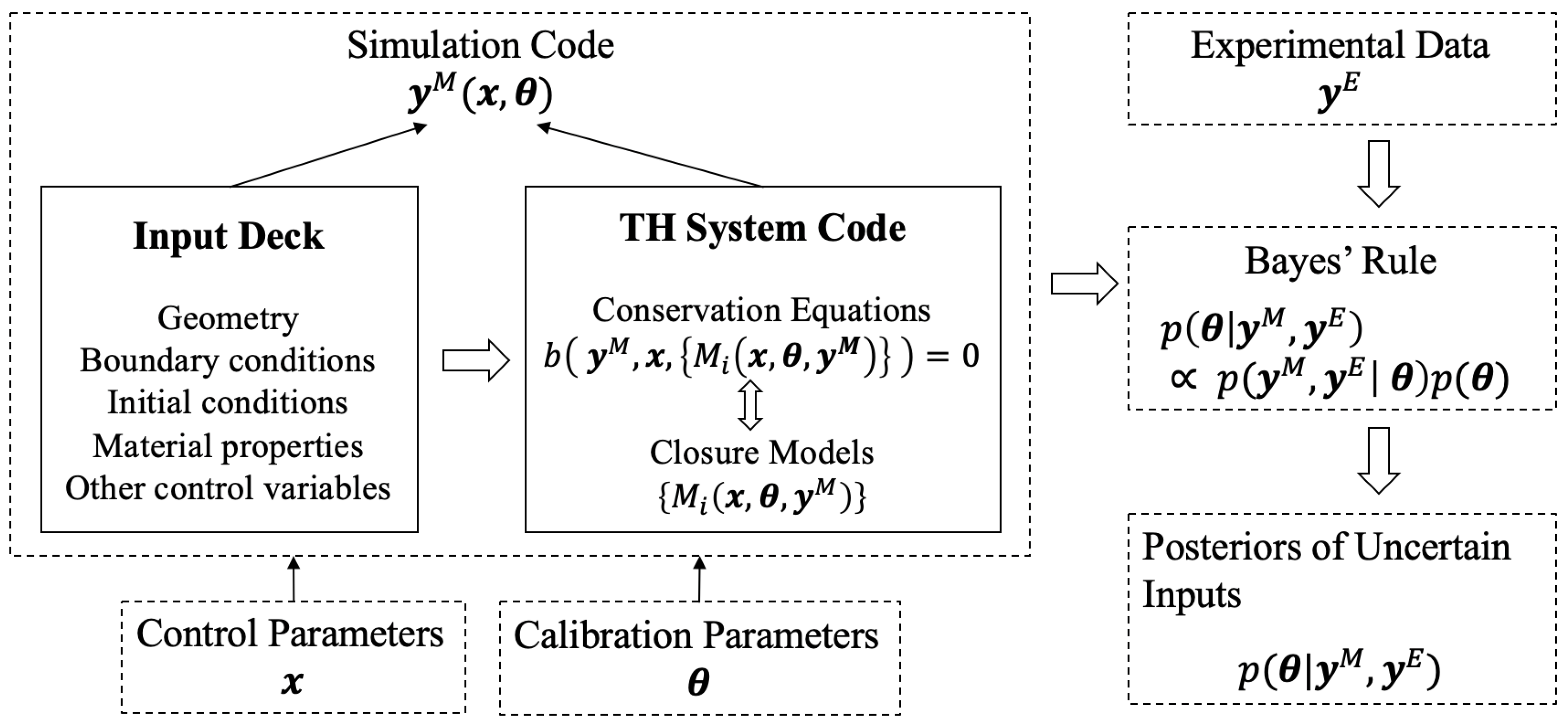
Figure 1. Key Elements of the IUQ framework [32].
Energies 16 07664 g001
Figure 2. Experimental facility for void fraction measurement in the BFBT benchmark [36].
Energies 16 07664 g002
Figure 3. Comparison of TRACE-predicted and experimentally-measured void fractions, assembly 4 in the BFBT benchmark.
Energies 16 07664 g003
Figure 4. Diagram of a hierarchical model.
Energies 16 07664 g004
Figure 5. Synthetic data example diagram.
Energies 16 07664 g005
Figure 6. Negative ELBO track for the synthetic data example.
Energies 16 07664 g006
Figure 7. KDE plots of the posterior distributions sampled by NUTS and ADVI algorithms and comparison with true values.
Energies 16 07664 g007
Figure 8. Hierarchical Bayesian model of the TRACE/BFBT application.
Energies 16 07664 g008
Figure 9. Surrogate model performance on validation dataset.
Energies 16 07664 g009
Figure 10. Comparison of the hyper-parameters’ posterior distributions by NUTS and ADVI methods.
Energies 16 07664 g010
Figure 11. Comparison of the posterior distributions of total variance  σ t  by NUTS and ADVI methods.
Energies 16 07664 g011
Figure 12. Correlations between two pairs of hyper-parameters, ( μ P 1008 μ P 1012 ) and ( μ P 1022 μ P 1028 ), using bivariate KDE plots.
Energies 16 07664 g012
Figure 13. Comparison of the PMPs’ posterior distributions by ADVI and NUTS methods.
Energies 16 07664 g013
Figure 14. Comparison of simulation results among (1) original model; (2) updated model using posteriors obtained by ADVI; and (3) updated model using posteriors obtained by NUTS. The error bars represent the 2.5–97.5 percentile of the model QoIs obtained from the FUQ step, using the posterior distributions of the PMPs that have been quantified during IUQ.
Energies 16 07664 g014
Table 1. Computing time comparison of ADVI and NUTS methods for the synthetic data example.
ADVINUTS
Number of fitting/sampling steps required120,0006000
Computational time12 s50 s
Table 2. List of 4 selected PMPs in TRACE.
ParameterDefinition
  P 1008 Single phase liquid to wall heat transfer coefficient
  P 1012 Subcooled boiling heat transfer coefficient
  P 1022 Wall drag coefficient
  P 1028 Interfacial drag (bubbly/slug Rod Bundle–Bestion) coefficient
Table 3. Prior distributions of the hyper-parameters in the hierarchical model.
ParametersDistributionsDist. Parameter 1Dist. Parameter 2
  μ P 1008 , μ P 1012 , μ P 1022 , μ P 1028 Uniform   a = 0   b = 3
  σ P 1008 , σ P 1012 , σ P 1022 , σ P 1028 Uniform   a = 0   b = 1
  σ t Normal   μ = 0   σ = 1
Table 4. Fitted distributions from the posteriors of PMPs.
ParametersNUTSADVI
  P 1008   μ = 1.63   σ = 0.66   μ = 1.34   σ = 0.49
  P 1012   μ = 1.32   σ = 0.18   μ = 1.45   σ = 0.21
  P 1022   μ = 0.89   σ = 0.12   μ = 0.89   σ = 0.33
  P 1028   μ = 1.26   σ = 0.15   μ = 1.32   σ = 0.22
Table 5. Computing time comparison of ADVI and NUTS methods for TRACE BFBT application.
ADVINUTS
Number of fitting/sampling steps required300,000100,000
Computational time58 s1520 s
Disclaimer/Publisher’s Note: The statements, opinions and data contained in all publications are solely those of the individual author(s) and contributor(s) and not of MDPI and/or the editor(s). MDPI and/or the editor(s) disclaim responsibility for any injury to people or property resulting from any ideas, methods, instructions or products referred to in the content.