Abstract
For the sake of conducting distribution network reliability prediction in an accurate and efficient manner, a model for distribution network reliability prediction (IAO-LSSVM) based on an improved Aquila Optimizer (IAO) optimized mixed-kernel Least Squares Support Vector Machine (LSSVM) is thus proposed in this paper. First, the influencing factors that greatly affect the distribution network reliability are screened out through grey relational analysis. Afterwards, the radial basis kernel function and polynomial kernel function are combined and a mixed kernel LSSVM model is constructed, which has better generalization ability. However, for the AO algorithm, it is easy to fall into local extremum. In such case, the AO algorithm is innovatively improved after both the improved tent chaotic initialization strategy and adaptive t-distribution strategy are introduced. Next, the parameters of the mixed-kernel LSSVM model are optimized and the IAO-LSSVM distribution network reliability prediction model is established through using the improved AO algorithm. In the end, the prediction results and errors of the IAO-LSSVM prediction model and other models are compared in the actual distribution network applications. It is revealed that the IAO-LSSVM prediction model proposed in this paper features higher accuracy and better stability.
1. Introduction
As an essential part of the power system, the power distribution network features a wide range and complex structure, which have an important impact on the reliability of the distribution network. In consequence, it is of great importance to predict the power supply reliability of the distribution network accurately and effectively [1].
There are three most commonly used reliability prediction methods for distribution networks: the simulation method, analytical method, and artificial intelligence algorithm. For the simulation method, the Monte Carlo method is the most commonly used. Although it has high calculation accuracy, the Monte Carlo method has the shortcoming of long calculation time, which means it is difficult to meet the needs of online analysis [2]. The most commonly used analytical methods include the network equivalent method [3], failure mode analysis method [4], and minimum cut set method [5]. However, these three methods are complex in calculation while poor in generality. Neural networks are non-parametric data-driven methods. In reference [6], the Mind Evolutionary Algorithm (MEA) was proposed to optimize and improve the reliability prediction model of distribution networks based on Elman neural networks. Experimental results demonstrated the improved accuracy of this method. However, there may be issues such as local minima and overlearning in practical applications. In reference [7], the Improved Particle Swarm Optimization (IPSO) algorithm was suggested to optimize the reliability prediction model of distribution networks, based on the Generalized Regression Neural Network (GRNN). IPSO was utilized to optimize the parameters of GRNN. However, the accuracy of the prediction model cannot be guaranteed when training data samples are limited. Reference [8] proposed the Support Vector Machines (SVM) as a machine learning algorithm based on small sample statistical learning theory. It overcame the drawbacks of neural networks by minimizing structural risk and achieved high prediction accuracy even when the data samples are limited. However, the standard SVM requires solving quadratic programming equations, which results in high computational complexity and slow speed. The Least Squares Support Vector Machine (LSSVM) algorithm is a machine learning algorithm specifically designed for small sample situations. Reference [9] proposed combining the structural risk minimization criterion with least squares estimation, which transformed the quadratic programming solution in standard SVM into linear equation solving, simplifying the computation process, increasing the operation speed, and solving the overfitting and underfitting problems of neural networks. This provides a new research method for reliable prediction of small sample power distribution network. Traditional LSSVM models often use a single kernel function, yet each kernel function has its own limitations that can affect prediction accuracy to some extent. Mixed-kernel LSSVM models combine different kernel functions through weighted combinations, which can balance the strengths of multiple kernel functions and achieve better prediction accuracy and generalization performance than single-kernel LSSVM models. However, compared to single-kernel LSSVM, mixed-kernel LSSVM models have more parameters and are more difficult to determine. References [9,10,11] have used particle swarm optimization (PSO) and the genetic algorithm (GA) to search for optimal parameters for mixed-kernel LSSVM models. Adaptive optimization (AO), as a novel swarm intelligence algorithm, has been proven to have strong global optimization ability with simple structure and better optimization efficiency than other algorithms such as GA and PSO [12].
In summary, this article proposes a global optimization method for hybrid kernel LSSVM parameters using an improved eagle-inspired optimizer (IAO). Based on this, a reliability prediction model for distribution networks using mixed kernel IAO-LSSVM is established and compared with other optimization models in terms of reliability, prediction results, and errors. The results show that the mixed kernel IAO-LSSVM model has smaller prediction errors and higher accuracy, providing certain reference significance for the future planning of distribution networks.
2. Aquila Optimizer and Its Improvements
2.1. Aquila Optimizer (AO)
As a latest novel swarm intelligence optimization algorithm, the Aquila Optimizer (AO) was inspired by the behavior of Aquila in nature. AO has two phases, namely exploration and exploitation. If , the exploration steps will be executed; otherwise, the exploitation steps will be executed. The exploration steps are divided into expanded exploration and narrowed exploration while the exploitation steps are divided into expanded exploitation and narrowed exploitation. First, AO starts by determining the initial value for a set of N individuals X through the following formula:
In the above Equation (1), is a random number between [0,1], i = 1, 2, N, j = 1, 2, d, N is the total number of candidate solutions (population), d is the dimension of the test problem, LBj and UBj denote the lower bound and upper bound at dimension j, respectively.
2.1.1. Expanded Exploration
In this phase, the Aquila flies high over the ground and explores the search space widely, and then a vertical dive will be taken once the area of the prey is determined. The mathematical representation of this behavior is written as follows:
In the above Equation (2), rand is a random value between 0 and 1, K is the number of total iterations, Xbest(k) is the best-obtained solution until kth iteration, XM(k) denotes the locations mean value of the current solutions connected at kth iteration, and it is computed as follows:
wherein, is the dimension size of the optimization variable.
2.1.2. Narrowed Exploration
The Aquila circles above the target prey when the prey area is found from a high soar, and then attacks. This behavior is mathematically presented as in Equation (4) below.
wherein, XR denotes a random chosen individual. Levy(d) is the levy flight distribution function, and it is calculated by Equation (5). d is the dimension size. y and x represent the spiral shape in the search. The calculations are as follows in Formulas (6) to (9):
wherein, s and are equal to 0.01 and 1.5, respectively, while u and v are random numbers between 0 and 1. As a random value, r1 is between 0 and 20. d1 is integer numbers from 1 to the length of the search space (d). U = 0.00565 and are small values.
2.1.3. Expanded Exploitation
When the prey area is specified accurately, the Aquila descends vertically for a preliminary attack to discover the prey reaction. It is mathematically represented as in Equation (10).
wherein, rand is between 0 and 1; and are 0.1. LB denotes the lower bound and UB denotes the upper bound of the search space.
2.1.4. Narrowed Exploitation
When the Aquila draws close to the prey, it attacks the prey over the land in light of its stochastic movements. The mathematical representation of this behavior is written as in Equation (11).
wherein, QF is used to balance the search strategy, see Formula (12) for the calculation. G1 and G2 refer to Formulas (13) and (14), respectively.
2.2. Improved Aquila Optimizer (IAO)
Compared with other swarm intelligence optimization algorithms, AO not only has high optimization accuracy, but also fast convergence speed [12]. Nevertheless, just like other optimization algorithms, the population diversity of AO will also decrease at the later iteration, and local optimal problems will appear. Therefore, an improved AO is proposed in this paper. First of all, the improved tent chaotic mapping is utilized to initialize the population so as to improve the global search ability of the algorithm. Then, the adaptive t-distribution strategy is introduced for the position update, which effectively improves the defect that it is easy to fall into local extremum. The improved strategy is as below:
- Improved tent chaos mapping
Random generation is used in AO to initialize the population, leading to uneven distribution of the Aquila population. Chaotic mapping is characterized by regularity and ergodicity [13], so in this paper, chaotic sequencing is used to initialize the position of the Aquila. The most commonly used chaotic mappings are logistic mapping and tent mapping. As can be seen from Figure 1a, the distribution probability of logistic mapping values is higher between [0,0.1] and [0.9,1], and this inhomogeneity seriously affects the optimization efficiency of the algorithm. It can be observed from Figure 1b that it is more uniform in tent mapping distribution.

Figure 1.
Distribution histogram of different chaotic sequences. (a) Logistic chaotic sequence distribution histogram. (b) Tent chaotic sequence distribution histogram. (c) Improved tent chaotic sequence distribution histogram.
The tent mapping function is calculated as follows: Formula (15)
The expression after the Bernoulli transformation is as shown below:
Tent chaotic sequencing has the problem that it will fall into small periodic points and unstable periodic points during iteration [14]. Hence, a random variable (0,1)(1/NT) is added to the original, and the expression is as follows:
The expression after the Bernoulli transformation is as shown below:
wherein, NT represents the number of particles in the chaotic sequence, while rand (0,1) represents the random number between (0,1).
In this paper, an improved tent chaotic mapping is adopted to initialize the population, rendering the position distribution of the initial population more uniform. The steps are as below:
- Generate a random number x0 between (0,1), = 0.
- As in Equation (18), an sequence is generated, and increases by 1
- When i reaches the maximum number of iterations, the sequence is saved
- As shown in Formula (19), the elements of sequence are mapped to the Aquila individual so as to obtain
- Wherein, UB and LB represent the upper and lower bounds of the search space, respectively.
- 2.
- Adaptive t-distribution strategy
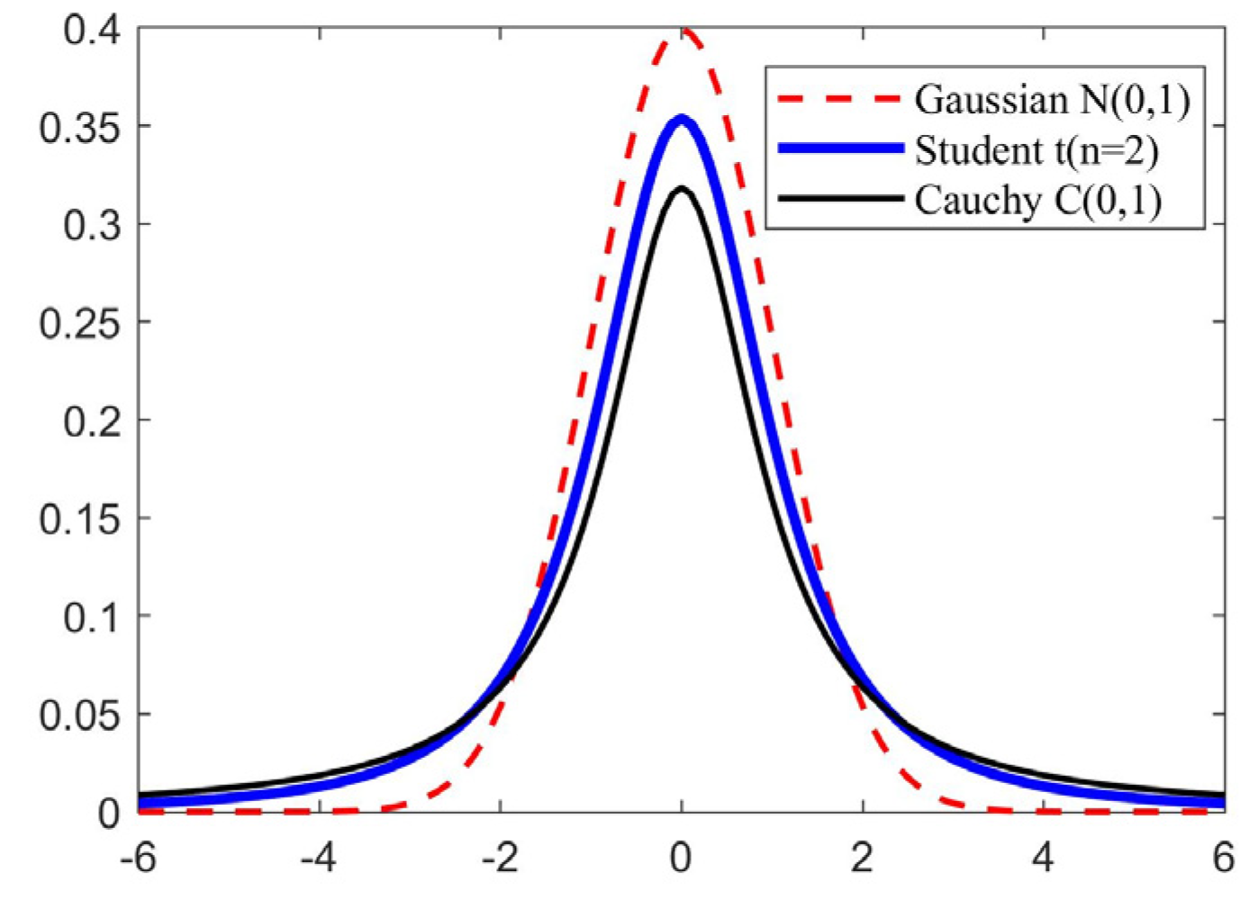
T-distribution is also known as student distribution [15]. The shape of the distribution function curve is up to the value of the parameter degree of freedom n. As indicated in Figure 2, the smaller the degree of freedom n is, the flatter the shape of the curve is. If the degree of freedom n = 1, the t-distribution is similar to Cauchy distribution, expressed as t(n = 1)→C(0,1). The larger the degree of freedom n is, the higher the curve shape is, and the curve is close to the standard normal distribution curve. When the degree of freedom n is infinite, the t-distribution is like the Gaussian distribution, expressed as t(n = )→N(0,1).
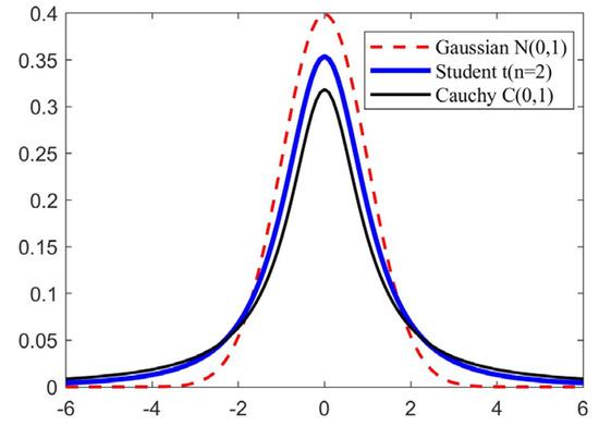
Figure 2.
Distribution map of t distribution, Gaussian distribution, and Cauchy distribution function.
The adaptive t-distribution is used for the Aquila’s position update, as shown in the following formula:
wherein, represents the Aquila’s position after t variation, xi is the position of the ith Aquila individual, and t(k) indicates that in the t-distribution the current iteration number is selected as the parameter freedom. When the current iteration number k becomes smaller, the t-distribution is alike to the Cauchy distribution variation. In this case, the t-distribution operator obtains a larger value, and the step size of the position variation becomes larger, which means the algorithm has a better global search ability. During the middle of iteration, in t-distribution, it changes from Cauchy distribution variation to Gaussian distribution variation, and the t-distribution operator’s value is relatively in the middle. In the algorithm combining the advantages of the two, it has both global and local search ability. When the number of iterations k is larger during the later iteration, the t-distribution is similar to Gaussian distribution variation. At this point, the t-distribution operator’s value and the variation step are both smaller, which means the algorithm has better local search ability. This strategy is beneficial to finding the global optimal point in the algorithm.
2.3. IAO Performance Evaluation
2.3.1. Parameter Setting and Benchmarking Function Selection
In a bid to verify the performance of the IAO algorithm, GA [16], PSO [17], GWO [18], SSA [19], AO, and IAO are employed to conduct simulation experiments on the test function. The parameter settings of each algorithm are outlined in Table 1, and each algorithm has a population size of 30. The multi-dimensional single-peak function Sphere and multi-dimensional multi-peak function Ackley are selected for the benchmarking function, and the dimensions d of each function are 10, 30, and 100 dimensions, respectively. The value range and optimal solution information of the test function are shown in Table 2.

Table 1.
Parameter setting table.

Table 2.
Benchmarking function.
2.3.2. Comparative Analysis of Algorithm Performance Results
The Sphere and Ackley benchmark test functions were optimized using GA, PSO, GWO, SSA, AO, and IAO algorithms. Table 3 shows the results obtained by independently running these four algorithms twenty times, yielding the average and standard deviation for each. By comparing the average and standard deviation, the precision and stability of each algorithm can be reflected. The closer the value is to 0, the higher the algorithm’s stability.

Table 3.
Comparison of test function optimization results.
In the multi-dimensional single-peak function Sphere, as dimensionality increases, the optimization accuracy of GA, PSO, GWO, SSA, and AO noticeably decreases because these algorithms tend to get stuck in local optima, making them unsuitable for high-dimensional problems. In contrast, the improved IAO algorithm, which incorporates tent map chaos initialization and adaptive t-distribution strategy, enhances its ability to escape local optima and perform global optimization. As a result, the optimization accuracy of the IAO algorithm is further improved with increasing functional dimensionality. Compared to the other five algorithms, the IAO algorithm exhibits extremely high optimization precision and greater stability, with both mean and standard deviation being the smallest. This observation holds true for the multi-dimensional multi-peak function Ackley as well, where the optimization accuracy of GA, PSO, GWO, SSA, and AO still decreases with dimensionality, but the mean and standard deviation of IAO hardly change and remain the smallest, which further demonstrates its superiority over the other five algorithms in terms of optimization accuracy and stability.
2.3.3. Comparative Analysis of Algorithm Convergence Curves
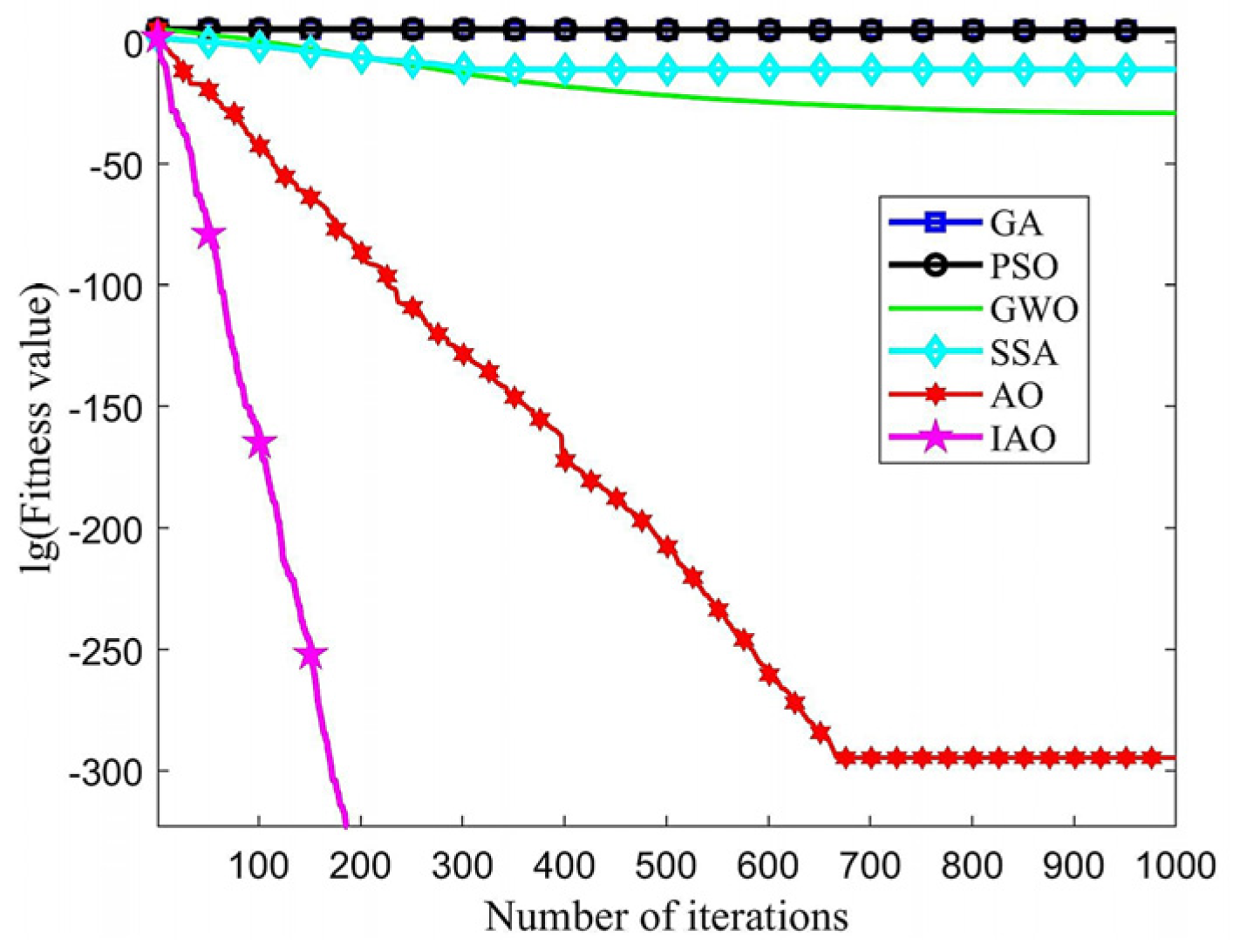
Under the same operating conditions, each algorithm had a population size of 30 and a maximum iteration of 1000, and each algorithm runs independently 20 times. The convergence curves of GA, PSO, GWO, and SSA, AO, IAO on two test functions (d = 30) are shown in Figure 3 and Figure 4, respectively. The x-axis represents the iteration number, while the y-axis represents the logarithm of the fitness value (i.e., lg(fitness value)). The fitness value here refers to the value of the test function. The benchmark test function curves can clearly demonstrate the algorithm’s convergence speed, accuracy, and ability to escape local spaces. The earlier the curve appears to change direction, the faster the convergence speed. The lower the lg(fitness value), the higher the optimization accuracy.
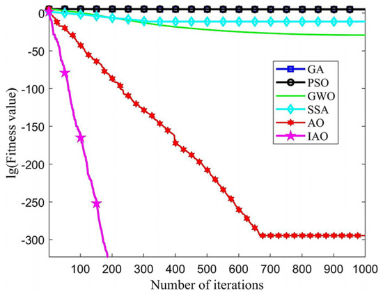
Figure 3.
Sphere function optimization curve.
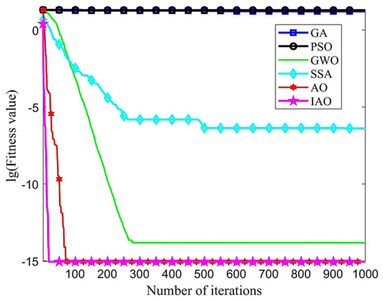
Figure 4.
Ackley function optimization curve.
The convergent curves of GA, PSO, GWO, and SSA in the optimization process are relatively gentle, with slow inflection point occurrence. Therefore, these four algorithms tend to become stuck in local optima early on in the iteration process and cannot escape with increasing iterations, resulting in poor convergence effectiveness and optimization accuracy. Compared to AO and other algorithms, IAO has a faster downward curve and inflection point appearance. Thus, IAO outperforms the aforementioned algorithms in terms of optimization accuracy and convergence speed.
3. Mixed Kernel IAO-LSSVM Prediction Model
3.1. Mixed Kernel LSSVM Model
The distribution network reliability data are based on each year and have a small quantity of data; LSSVM has advantages in dealing with regression problem of small samples [20]. So, in this paper LSSVM is used to achieve reliability prediction of the distribution network. First proposed by Suykens et al. [9]. LSSVM is an improved SVM featuring simpler and faster computation.
It is assumed that the sample set (xi, yi) of the reliability training data of the distribution network is obtained, where i = 1, 2… l, xi ∈ Rn is the n-dimensional input, yi ∈ R is the one-dimensional output, xi represents the influence factor data on distribution network reliability [21], and yi indicates the reliability index data of the distribution network. When the Least Square Support Vector Machine (LSSVM) is used to process such regression problems as the reliability prediction of distribution networks, the nonlinear problems in the original low-dimensional space are transformed into linear regression in the high-dimensional space by means of nonlinear mapping function [22], that is, in the high-dimensional space, the input and output of samples are fitted:
wherein w is the weight matrix and b is the offset quantity.
The principle of structural risk minimization is adopted in defining optimization problems:
In the formula above, C is the penalty parameter. The higher the value of C is, the more likely it is to be over-fitted; the lower it is, the more prone it is to be under-fitted. Therefore, it is necessary to make a reasonable choice of C. ei is the fitting error.
Then, use the Lagrange function to solve the optimization problem as below:
wherein, is the Lagrange multiplier.
Based on the condition of KKT, the partial derivative of Equation (23) is equal to 0, and then
Next, define the kernel function K(xi, xj) = φ(xi)φ(xj) which satisfies the Mercer principle, the necessary and sufficient conditions of the kernel function, and then the prediction model can be expressed as follows:
The performance of LSSVM is determined by kernel function. As for the traditional kernel functions, as a global kernel function, the polynomial kernel function has poor local learning ability. As a local kernel function, the radial basis kernel function (RBF) has good local learning ability. Therefore, the advantages of the two kernel functions are combined to construct a mixed kernel function:
wherein, λ is the weight coefficient and λ ∈ [0,1], q represents the parameters of the polynomial kernel function and means the parameters of the radial basis kernel function.
3.2. Establishment of Mixed Kernel IAO-LSSVM Model
For the establishment of the mixed kernel LSSVM distribution network reliability prediction model, the grey relational analysis method [23] is used to analyze the correlation degree of the influencing factors. The influencing factors with a correlation degree higher than a set threshold value are selected as the input of the model. This reduces the complexity of model training and the calculation time. However, for the prediction accuracy of the mixed kernel LSSVM model, parameters C, , q and are the determining factors, so parameter optimization is particularly important.
In this paper, in order to optimize the parameters, the improved Aquila Optimizer is used, where each Aquila represents a set of parameters (C,,q,). The specific modeling steps are as follows:
- Initialize the parameters. Set the optimization intervals of C, λ, q, and , as well as relevant parameter values of the IAO algorithm. Formulas (18) and (19) are adopted to initialize the Aquila population.
- Select the fitness function. The MSE of the predicted value and the true value of the training sample are taken as the fitness value of the Aquila individual, where is calculated by Formula (25). The calculation formula of MSE is as shown below:
- 3.
- The fitness values of Aquila individuals are calculated, based on what current best position Xbest(k) is determined. XM(k), G1, G2, Levy(d) are updated
- 4.
- When k ≤ (2/3)K and rand ≤ 0.5, refer to the Formula (2) for the location update of the Aquila individual; otherwise, refer to the Formula (4).
- 5.
- When (2/3)Kk ≤ K, and rand ≤ 0.5, the Formula (10) is used to update the location of the Aquila individual; otherwise, the Formula (11) will be used.
- 6.
- In accordance with Equation (20), the t-distribution mutation operation is conducted on the Aquila position.
- 7.
- Calculate the fitness value of each Aquila after t-distribution variation. Update individual fitness values as well as global optimal information.
- 8.
- Termination condition. The parameters corresponding to the optimal Aquila individual position (C,,q,) are output if the maximum number of iterations K has been reached. Thus, the mixed kernel IAO-LSSVM distribution network reliability prediction model is established. Otherwise, return to Step 3
- 9.
- The grey relational analysis method is used for analyzing the data. Firstly, the distribution network data are processed in a dimensionless manner. Secondly, the entropy weight correlation degree of influencing factors of power supply reliability is calculated. Finally, the influencing factors are sorted in accordance with the grey correlation degree, and the entropy weight correlation degrees higher than the set threshold are selected as the input of the mixed kernel IAO-LSSVM model.
- 10.
- Data set division. The influencing factors selected in step 9 are taken as the input of the model, while the distribution network reliability index is taken as the output of the model. Then, the distribution network reliability data are divided into training set and test set, and are normalized.
- 11.
- The established mixed kernel IAO-LSSVM model is used for the distribution network reliability prediction.
3.3. Model Evaluation Index
Root Mean Square Error (RMSE), Mean Absolute Percentage Error (MAPE), and Mean Absolute Error (MAE) are selected as the evaluation indexes of the model so as to compare the performance of each model. The calculation formulas of each index refer to Formulas (28), (29), and (30), respectively.
wherein, represents the predicted value, indicates the real value, and is the total number of data samples for model performance testing.
4. Case Analysis
The distribution network reliability data of Hubei Province from 2006 to 2015 [6] are selected for the experiment, and the distribution network reliability index involves power supply reliability. Refer to Table 4 for 27 power supply reliability rates and influence factor data of the Hubei power distribution network from 2006 to 2015, and Table 5 for the result table of the entropy weight correlation degree of influencing factors of the power supply reliability rate of the distribution network in Hubei Province.

Table 4.
Power supply reliability rate and influence factor data of the Hubei power distribution network from 2006 to 2015.

Table 5.
Result table of entropy weight correlation degree of influencing factors of power supply reliability rate of the distribution network in Hubei Province.
4.1. Analyze Influencing Factors
The entropy weight-grey correlation analysis method is used to calculate the entropy weight correlation degree of each influencing factor X1–X27 relative to the power supply reliability indicator X0. The size of the entropy weight correlation degree reflects the degree of influence of each factor on the reliability indicator. The larger the entropy weight correlation degree, the closer the correlation between the two. Table 5 presents the entropy weight correlation degrees of each influencing factor.
Among them, correlation degrees of entropy weight greater than 0.7 are called a strong correlation factor, while those below 0.3 are weak. Therefore, in this paper, the influencing factors with a correlation degree of no less than 0.7 are selected as the input of the model. The influencing factors X9 and X27 are rejected, and the remaining 25 influencing factors are chosen as the input of the model, while the power supply reliability X0 is taken as the output of the model.
4.2. Model Parameter Determination
The eight groups of data from 2006 to 2013 shown in Table 3 are used as training samples for power supply reliability prediction in 2014 and 2015 in order to verify the predictive performance of the IAO-LSSVM model. The accuracy of the same test set (all the combination models use the mixed-core LSSVM) is compared for the models including single-kernel RBF-LSSVM, mixed-core LSSVM, GA-LSSVM, PSO-LSSVM, GWO-LSSVM, SSA-LSSVM, AO-LSSVM, and IAO-LSSVM. For each optimization algorithm, the parameter settings are identical to those in the IAO performance evaluation, with dimensions d = 4 and K = 100. In the RBF-LSSVM model, the radial basis kernel function is selected, with parameters C = 100, = 5. For the mixed kernel LSSVM model, the mixed kernel function combining radial basis kernel function and polynomial kernel function is used, with parameters C = 100, λ = 0.5, q = 1, = 5. As for other model parameters C, λ, q, and , the lower and upper bounds are [100, 0, 0.7, 3] and [300, 1, 1.3, 5], respectively.
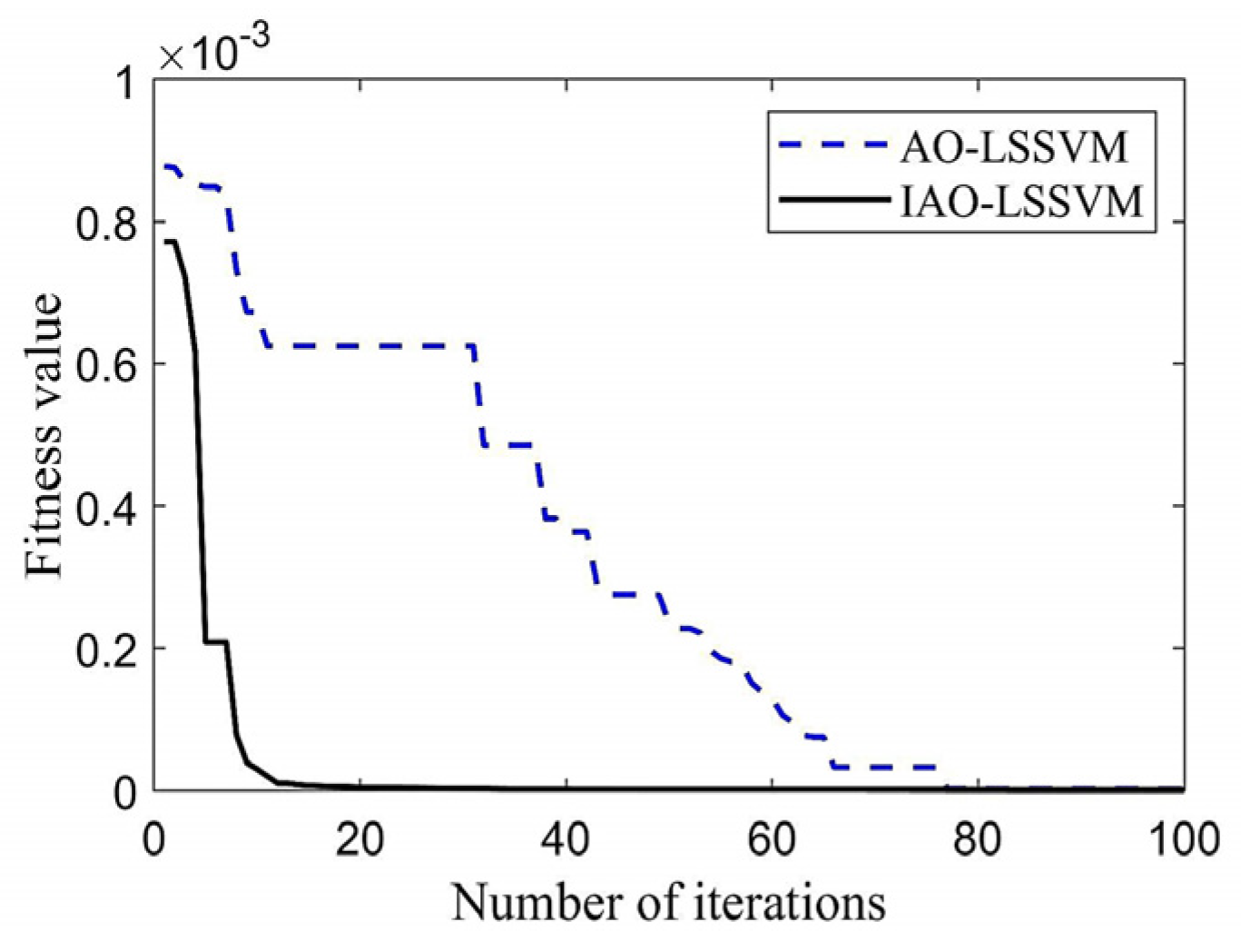
The fitness curves of IAO and AO optimized LSSVM refer to Figure 5. The ISSA-LSSVM curve shows a faster descent rate and a turning point, indicating that the model has faster convergence speed and better convergence accuracy, leading to better performance. Table 6 presents the optimization results of hybrid core LSSVM parameters.
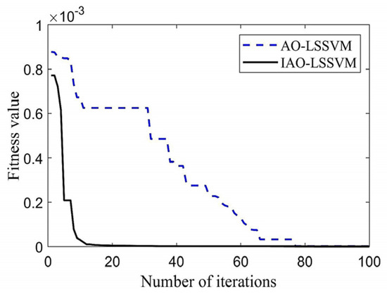
Figure 5.
AO-LSSVM and IAO-LSSVM model fitness curves.

Table 6.
Optimization results of hybrid core LSSVM parameters.
5. Discussion
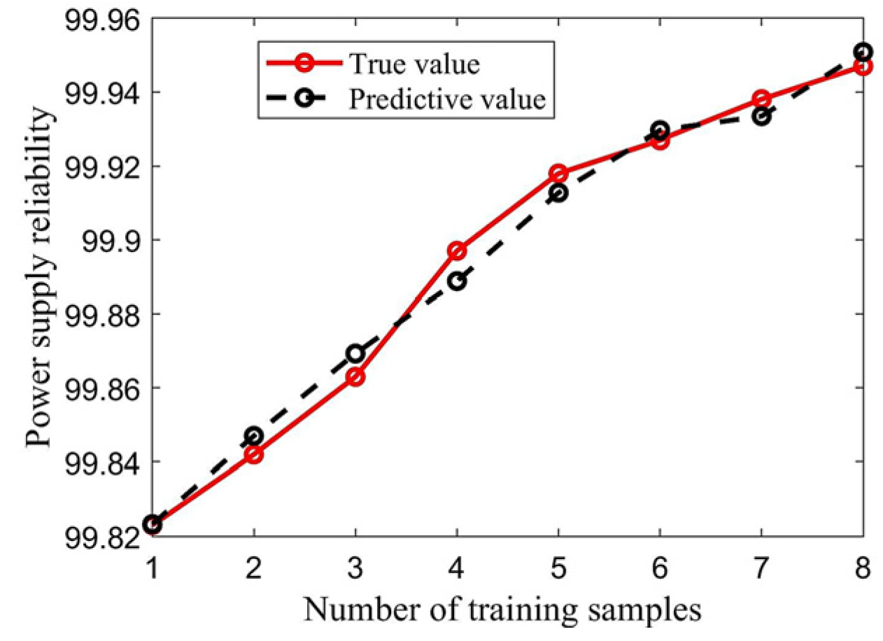
In experiment 1, a random selection of 9 years of samples from 2006 to 2015 was chosen for training in order to predict the reliability of power supply for a year outside of these samples. Figure 6 displays the comparison between the prediction results of the IAO-LSSVM model and the actual values of the training samples, which shows a high degree of agreement between the predicted and actual values. This proves that the model is capable of accurately predicting the reliability of distribution networks, and demonstrates the algorithm’s wide applicability for analyzing trends in reliability changes.
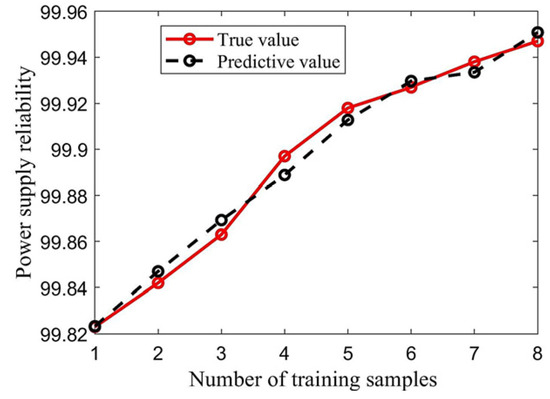
Figure 6.
Comparison of prediction results of training samples.
In experiment 2, eight samples from 2006 to 2013 were selected as training samples to predict power supply reliability in 2014 and 2015. The predictive effects of the RBF-LSSVM model, hybrid kernel LSSVM model, GA-LSSVM model, PSO-LSSVM model, GWO-LSSVM model, SSA-LSSVM model, AO-LSSVM model, and IAO-LSSVM model were compared with actual values. To provide a more intuitive display of the results, bar graphs of the predictive results and actual values for each model were created in the testing sample (as shown in Figure 7). Additionally, Table 7 lists three types of errors for the eight models when applied to the testing sample and time required to run the model.
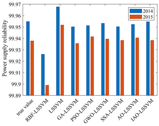
Figure 7.
Histogram of sample prediction results of each model.

Table 7.
Error comparison of test data and time required to run the model.
As can be seen from Figure 7, IAO-LSSVM has a good fitting degree for the training samples. The prediction accuracy of the IAO-LSSVM model for test samples is much higher than that of other models. For the error comparison in Table 5, it shows that the prediction error of IAO-LSSVM is the minimum among the eight models. The root mean square error (RMSE) of the three evaluation indexes are chosen to analyze the eight models. The RBF-LSSVM model with single kernel function has a maximum error of 0.0494. Compared with RBF-LSSVM, the mixed kernel LSSVM has a smaller error of 0.0241. As the parameters for these two models are obtained based on previous experience, certain errors still exist comparing with other optimized models. The IAO-LSSVM model among all the combination models has the minimum prediction error of 5.8567 × 10⁻⁵, which is one order of magnitude higher than others.
Therefore, it can be judged that the IAO-LSSVM prediction model demonstrates smaller error and higher accuracy than other common models in use, and it has achieved good results on power supply reliability prediction of the distribution network. The required running times for each algorithm’s prediction models are shown in Table 5, with the IAO algorithm requiring the shortest time compared to other algorithms. Therefore, it can be concluded that the IAO algorithm has a higher optimization speed compared to other algorithms and proves that the tent chaos initialization and adaptive t-distribution strategy have optimization effects on the convergence speed of the AO algorithm.
6. Conclusions and Future Work
In terms of problems needing to be solved, in the paper, the grey relational analysis method is firstly used to analyze the reliability data of distribution network. Then, the improved tent chaos initialization strategy and the adaptive t-distribution strategy are introduced to improve the AO algorithm, which enhances the searchability of the algorithm. Meanwhile, the parameters of the mixed kernel LSSVM model are optimized through the improved AO algorithm, and it effectively avoids blind parameter selection. In the paper, the distribution network reliability data come from fewer samples; however, their advantages are maximized due to the LSSVM model being used for reliability prediction. In terms of the prediction results, in this paper, the power supply reliability prediction results and errors of the RBF-LSSVM model, mixed kernel LSSVM model, GA-LSSVM model, PSO-LSSVM model, GMO-LSSVM model, SSA-LSSVM model, AO-LSSVM, and IAO-LSSVM are compared and analyzed. The findings show that the IAO-LSSVM prediction model features higher accuracy and also better stability.
Regarding future work, the LSSVM model adopted in this paper adopts a single radial basis kernel function, which has certain limitations, and the linear combination of the two kernel functions can be considered to form a mixed-kernel LSSVM model. By improving the model, the reliability of the distribution network can be accurately predicted, and the future development trend of the distribution network can be accurately judged, which provides certain reference significance for the future planning of distribution networks.
Author Contributions
This paper was a collaborative effort among all authors. All authors participated in the analysis, discussed the results, and wrote the paper. All authors have read and agreed to the published version of the manuscript.
Funding
This research received no external funding.
Data Availability Statement
Not applicable.
Conflicts of Interest
The authors declare no conflict of interest.
References
- Liu, M.; Luan, Y.; Lu, X.; Hu, J.L.; Wu, D. Summary of Power Supply Reliability Forecast of Distribution Network, Technology ed.; China Electric Power: Beijing, China, 2012; pp. 40–42. [Google Scholar]
- Munoz-Delgado, G.; Contreras, J.; Arroyo, J.M. Distribution Network Expansion Planning with an Explicit Formulation for Reliability Assessment. Trans. Power Syst. 2017, 99, 95–99. [Google Scholar]
- Billinton, R.; Wang, P. Reliability network equivalent approach to Distribution System Reliability Evaluation. IEEE Proc.-Gener. Transm. Distrib. 1998, 145, 149–153. [Google Scholar] [CrossRef]
- Billinton, R.; Billinton, J.E. Distribution System Reliability Indices. IEEE Trans. Deliv. 1989, 4, 561–568. [Google Scholar] [CrossRef]
- Yan, Z.; Zhangchao, C. Evaluation of a 35/10 kV Electric Distribution System Reliability Level. J. Shanghai Jiaotong Univ. 1995, 29, 198–201. [Google Scholar]
- Wang, Y.X.; Pan, X. Reality evaluation of distribution network based on improved-elman feedback dynamic neural network. Water Resour. Power 2019, 37, 177–180. [Google Scholar]
- Zhan, C.Y. Research on Model Optimization of Distribution Network Reliability Prediction; Anhui University of Science & Technology: Huainan, China, 2020. [Google Scholar]
- Liu, Q.; Lu, H.; Wang, Q.; Zhang, H.L. A regional traffic volume rolling prediction model based on support vector machine. J. Harbin Inst. Technol. 2011, 43, 138–143. [Google Scholar]
- Suykens, J.; Vandewalle, J. Least Squares Support Vector Machine Classifiers. Neural Process. Lett. 1999, 9, 293. [Google Scholar] [CrossRef]
- Dong, H.; Shi, L.S.; Zhao, P.C. Reliability Prediction of Urban Power Network Based on PSO-LSSVM Model. Proc. CSU-EPSA 2014, 26, 82–86. [Google Scholar]
- Deng, H.; Zhu, X.; Zhang, Q.; Zhao, J. Prediction of Short-term Pubic Transportation Flow Based on Multiple-kernel Least Square Support Vector Machine. J. Transp. Eng. Inf. 2012, 10, 84–88. [Google Scholar]
- Abualigah, L.; Yousri, D.; Abd Elaziz, M.; Ewees, A.A.; Al-Qaness, M.A.; Gandomi, A.H. Aquila Optimizer: A novel meta-heuristic optimization algorithm. Comput. Ind. Eng. 2021, 157, 107250. [Google Scholar] [CrossRef]
- Liu, L.; Sun, S.Z.; Yu, H.; Yue, X.; Zhang, D. A Modified Fuzzy C-means (FCM) Clustering Algorithm and its Application on Carbonate Fluid Identification. J. Appl. Geophys. 2016, 129, 28–35. [Google Scholar] [CrossRef]
- Zhang, N.; Zhao, Z.D.; Bao, X.A.; Qian, J.; Wu, B. Gravitational Search Algorithm Based on Improved Tent Chaos. Control. Decis. 2020, 35, 893–900. [Google Scholar]
- Chen, X.; Zhao, S.; Liu, F. Robust identification of Linear ARX Models with Recursive EM Algorithm Based on Student’s T-Distribution. J. Frankl. Inst. 2021, 358, 1103–1121. [Google Scholar] [CrossRef]
- Li, H.; Peng, Y.; Deng, C.; G, D.Q. Review of Hybrids of GA and PSO. Comput. Eng. Appl. 2018, 54, 20–28+39. [Google Scholar]
- Li, X.; Deng, D.; Liao, D.; Chen, J.H. A Review on Application of Particle Swarm Optimization in Electric Power Systems. Power Syst. Prot. Control. 2007, 23, 77–84. [Google Scholar]
- Mirjalili, S.; Mirjalili, S.M.; Lewis, A. Grey Wolf Optimizer. Adv. Eng. Softw. 2014, 69, 46–61. [Google Scholar] [CrossRef]
- Xue, J.; Shen, B. A Novel Swarm Intelligence Optimization Approach: Sparrow Search Algorithm. Syst. Sci. Control. Eng. Open Access J. 2020, 8, 22–34. [Google Scholar] [CrossRef]
- Zhang, J.; Tang, Z.H.; Gui, W.H.; Chen, Q.; Liu, J.P. Interactive image segmentation with a regression based ensemble learning paradigm. Front. Inf. Technol. Electron. Eng. 2017, 18, 1002–1021. [Google Scholar] [CrossRef]
- Allan, R.N.; Billinton, R. Bibliography on the application of probability methods in power system reliability evaluation. IEEE Trans. Power Syst. Publ. Power Eng. Soc. 1999, 14, 51–57. [Google Scholar] [CrossRef]
- Xiong, Y. Improved FCM-LSSVM Prediction Model for Penicillin Fed-batch Fermentation. Control. Eng. China 2017, 24, 2237–2242. [Google Scholar]
- Yuan, K.; Luo, P.; Wang, G.; Jin, D.M.; Yao, L.Y. A New Method of Power System False Data Attack Detection Based on Grey Analysis. Adv. Technol. Electr. Eng. Energy 2019, 38, 17–23. [Google Scholar]
Disclaimer/Publisher’s Note: The statements, opinions and data contained in all publications are solely those of the individual author(s) and contributor(s) and not of MDPI and/or the editor(s). MDPI and/or the editor(s) disclaim responsibility for any injury to people or property resulting from any ideas, methods, instructions or products referred to in the content. |
© 2023 by the authors. Licensee MDPI, Basel, Switzerland. This article is an open access article distributed under the terms and conditions of the Creative Commons Attribution (CC BY) license (https://creativecommons.org/licenses/by/4.0/).


