Article

Prediction of Thermal Conductivity of Litz Winding by Least Square Method and GA-BP Neural Network Based on Numerical Simulations

1
Wuhan Institute of Marine Electric Propulsion, Wuhan 430064, China
2
College of Civil Engineering, Tongji University, Shanghai 200092, China
*
Author to whom correspondence should be addressed.
Energies 2023, 16(21), 7295; https://doi.org/10.3390/en16217295
Submission received: 12 September 2023 / Revised: 11 October 2023 / Accepted: 23 October 2023 / Published: 27 October 2023
(This article belongs to the Section J2: Thermodynamics)

Abstract

:
This paper proposes a Litz winding numerical-simulation model considering the transposition effect, and uses the transient-plane-source method to verify the numerical-simulation method. In addition, numerical methods were adopted to further investigate the impact of filling rate and epoxy-resin type, and their combined effects, on thermal conductivity. To facilitate engineering design, the discrete data points were fitted using the least square method to obtain a straightforward and application-friendly polynomial empirical formula. On this basis, the GA-BP neural network was used to analyze the data in order to seek out more accurate prediction results for the entire data set. As a result, compared with the least square method, the error between the prediction result and the target value in the x direction was reduced by 87.04%, and the error in the z direction was reduced by 84.97%.

1. Introduction

Motors are widely used in the marine, automotive, and aerospace industries. With the rapid advancement in permanent magnet materials and high-speed bearing technology, the traditional low-torque-density motor has struggled to keep up with market demand in recent years [1,2]. As a result, new requirements for high power, high-torque-density motor designs have been put forth [3,4]. However, in high-frequency operation, the skin effect and proximity effect increase the winding resistance of the internal magnetic components and generate significant AC losses, which seriously limit the power output and efficiency of the motor [5,6,7]. Therefore, to ensure that the motor can still retain a low winding AC resistance at high frequencies and to increase motor efficiency, multi-bundle transposition-braided Litz winding is frequently employed in the motor stator winding structure [8,9].
To achieve high power density of the motor, it is often necessary to pay attention to the thermal field of the motor during design, which requires research into the heat-transfer performance of the Litz winding inside the motor [10]. However, as a composite material, the twisting and transposition of Litz winding are highly intricate, making prediction of its thermal conductivity challenging [11]. At present, there are three main methods for estimating the thermal conductivity of Litz winding: the equivalent-analysis method, the experimental-measurement method, and the finite-element-simulation-analysis method. The equivalent-analysis method uses the homogenization technique to recombine various materials in Litz winding to quickly estimate the thermal conductivity, and, due to the complexity of the transposition evaluation, parallel alignment is often used for prediction, ignoring the heat dissipation advantage brought by Litz winding transposition [12,13]. Michael et al. [12] presented a thermally equivalent circuit for the Litz winding considering transposition effects without an analytical solution to the proposed thermally equivalent circuit. Yi et al. [14] developed an analytical model considering the transposition effect to predict the equivalent thermal conductivity of windings, resulting in a 10–30% improvement in heat dissipation capacity compared to parallel-aligned Litz winding. Due to the complex and variable structure of Litz winding, the experimental measurement method has also been more widely used for the measurement of the thermal conductivity of Litz winding. Simpson et al. [15] used a steady-state heat flow meter for experimental measurements and compared the measurements with numerical simulations of a parallel-aligned structure and achieved good agreement. Wrobel et al. [16] performed thermal conductivity measurements for one-dimensional heat transfer using a liquid-cooled cold plate and a power resistor energized by a DC source, and found that the thermal conductivity was independent of the temperature in the analyzed temperature range. As for the finite-element-simulation-analysis method, many scholars [17,18,19] have calculated and studied the thermal conductivity of Litz winding from a two-dimensional perspective, even though it can save more time for finite element analysis, but ignoring the transposition efficiency, the calculation results have a large inaccuracy. Salinas Lopez et al. [20] made the thermal simulation time shorter by simplifying the model with a simplified mesh, while ensuring good accuracy. Yi et al. [14] introduced a three-dimensional simulation calculation model of the transposed structure, which better simulated the results of the thermal conductivity in real cases.
However, with the above three methods, the predicted model was a simplified model with a parallel arrangement, it required a more complicated formula to calculate the prediction, or it required a lot of calculation time for the simulation, and was not able to evaluate and predict the thermal conductivity more quickly or accurately in the actual motor design. Therefore, in this paper, a numerical-simulation model with a realistic transposition effect is proposed, and the transient-plane-source method is used to validate the numerical model, and the effects of filling rate and epoxy-resin type, and their combined effects, on the thermal conductivity in the direction of x and z are investigated under different working conditions. To facilitate the subsequent design and use, the least square method is used to fit the curve and surface of the single and double variable data, and a relatively simple empirical formula is used to predict the thermal conductivity. On this basis, the prediction of thermal conductivity is further optimized using the GA-BP (genetic algorithm-back propagation) neural network [21], which significantly reduces the error value and provides a reference for the following motor design.
The least squares method is a mathematical tool widely used in various fields of data processing [22], such as error estimation, uncertainty, system identification, and prediction; the GA-BP neural network is a biological intelligence-optimization algorithm. It is essentially a global search technique for finding the optimal value. The genetic algorithm selects a certain number of possible solutions as a population based on randomly generated possible outcomes and obtains the optimal solution through population iteration according to corresponding rules, such as natural-genetic-selection and cross-mutation methods.

2. Method

2.1. Physical Model

Litz winding consists of multiple strands of copper wire twisted together [23], while each strand of copper wire (shown in Figure 1g) is obtained by braiding 23 transposed Litz wires. Since the braiding process of 23 Litz wires is difficult to estimate, for numerical simulation, the rolling is simplified to a single-strand copper wire with the same cross-sectional area [24]. Figure 1a presents a cross-sectional view of Litz winding with a 9-strand transposed copper wire in the center, and epoxy resin is used as an impregnating material to wrap around the copper wire in order to discharge air to enhance thermal conductivity. In the cross-section, the dimension in the x direction is L ( mm ), while the dimension in the z direction is H ( mm ). Thus, the filling rate of Litz winding can be simplified as A c o p p e r H L , where A c o p p e r = 149.8 mm 2 denotes the total area of the cross-section of 9 strands of copper wire. Figure 1b demonstrates the three-dimensional spatial structure of the copper wire of the Litz winding within four turns. The copper wire is freely arranged in Litz winding by stranding with a particular machine, and Figure 1c–f shows the transposition effect of the 9-strand copper wire. When the Litz winding is long enough, each strand of copper wire occupies every position on the Litz winding section, that is, each strand of copper wire occupies the position of other copper wires on a certain space segment.

2.2. Materials

The materials used for Litz winding are mainly copper wire and epoxy resin, and their material properties and parameters are shown in Table 1.

2.3. Simulation Method

Heat transfer can be defined as the exchange of internal energy between two objects in complete contact or between different parts of an object due to a temperature gradient, and its heat transfer follows Fourier’s law [25]:
q * = λ n m T n
where q * ( W / m 2 ) is the heat flow density, λ n m ( W / ( m K ) ) is the thermal conductivity, and T n is the temperature gradient along the heat-flow transfer direction. In finite-element analysis, the controlling differential equation for heat conduction is obtained by applying the first law of thermodynamics to a micro-element:
x λ x x T x + y λ y y T y + z λ z z T z + q = ρ c d T d t
where λ x x , λ y y , λ z z ( W / ( m K ) ) is the thermal conductivity in x , y , z direction, ρ ( k g / m 3 ) is the density of the material, c ( J / ( k g K ) ) is the specific heat of the material, T ( K ) is the temperature of the object, and t ( s ) is the time parameter. And to solve the above differential equation, boundary conditions are also required. There are three types of boundary conditions for heat transfer: 1. uniform temperature distribution on the boundary, 2. constant heat transfer on the boundary, and 3. the temperature of the surrounding medium and the heat-transfer coefficient on the boundary are known. The first type of boundary condition is used in the Litz winding thermal conductivity solution, on the boundary Γ :
T ( x , y , z , t ) = T 0
To solve the above heat-conduction problem, the problem can be described in the following equivalent variational form, and then the finite-element equations for solving such problems can be derived. To find the temperature distribution T ( x , y , z , t ) within the solid, the following function should be minimized:
Π = 1 2 V λ x x T x 2 + λ y y T y 2 + λ z z T z 2 2 q ρ c T t T d V
Within each cell, the temperature of each point can be approximately expressed by interpolation of the node temperature of the cell as follows:
T = i = 1 p N i ( x , y , z ) T i e = N T ( e )
In order to obtain the extreme value of Function (4), the necessary conditions should be satisfied:
Π T i = e = 1 E Π ( e ) T i = 0 ,   ( i = 1 , 2 , M )
where M is the total number of node temperature unknowns, and the finite-element equilibrium equation of each element can be obtained as follows:
K ( e ) T ( e ) = P ( e )
where K ( e ) is the overall thermal conductivity matrix, T ( e ) is the temperature array formed by solving the temperature of all nodes in the domain, and P ( e ) is the temperature load array. By solving the balance Equation (7), numerical-simulation results can be obtained.

2.4. Grid Independence Test

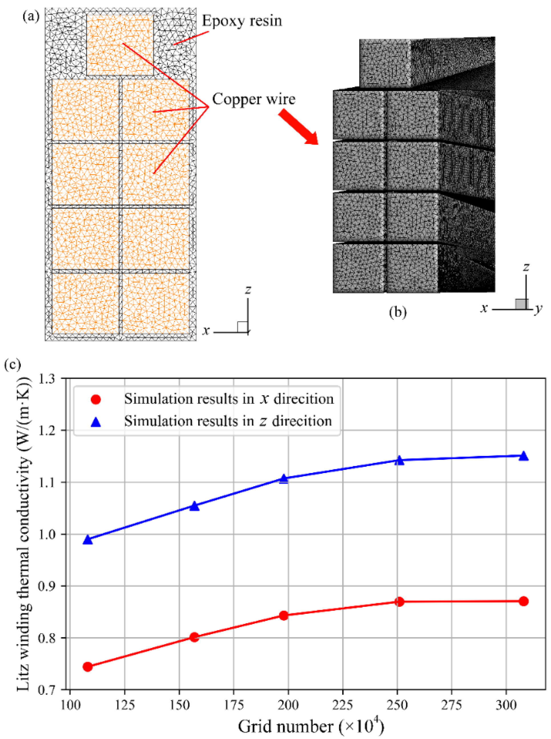
As depicted in Figure 2, considering the complexity of Litz winding transposition, all models calculated in this paper use unstructured grids. Five grid numbers, namely 108 × 104, 157 × 104, 198 × 104, 251 × 104, and 308 × 104, were utilized for grid-independent verification before numerical simulation. From Figure 2c, it can be concluded that the growth of the thermal conductivity in the x and z directions decreases as the number of grids increases. When the grid number is greater than 251 × 104, the thermal conductivity in x and z directions does not change much, and when the grid number changes from 251 × 104 to 308 × 104, the relative change rate of thermal conductivity in x direction is less than 0.44%, while the relative change rate of thermal conductivity in z direction is less than 0.58%, which can better meet the design requirements. Therefore, considering the accuracy and computation time, a grid number of 251 × 104 were used for numerical simulation and exploration in this study.

3. Experimental Verification

To further verify the correctness of the numerical model, the thermal conductivity of different specifications of Litz winding was measured to explore the consistency between the numerical-simulation results and the test results.

3.1. Sample Parameters

Table 2 shows the specifications and epoxy-resin properties of the Litz winding samples used in the experiments. Between different Litz windings, the specifications and properties of the copper conductors used were the same, and only the filling rate and material properties of the epoxy resin outside the copper conductors were changed. Usually, due to the limitation of motor space, the epoxy-resin material properties and filling rate need to be strictly calculated and controlled, but in order to thoroughly verify the rationality of the numerical model, three groups of representative filling rates and epoxy-resin types among the commonly used Litz winding parameters were selected for exploration in this experiment.

3.2. Hardware Setup and Test Procedure

Considering the size of the specimen and the range of thermal conductivities, the transient-plane-source method was used to measure thermal conductivity [26]. The transient-plane-source method was developed on the basis of the hot wire method to detect the thermal physical properties of materials, and uses a temperature-rise probe formed by the etching of a conductive metal (usually nickel) for measurement [27]. When the current passes through the probe, heat is generated, and the probe acts as both a heat source and a temperature sensor. Thus, the thermal conductivity of the material can be obtained by recording the temperature change and the response time of the probe. As illustrated in Figure 3a, the transient-plane-source measurement instrument consisted of a TPS controller (CTPS-2500 type, Tianjin Foreda Technology Co., Ltd., Tianjin, China), a test bench, and a laptop with thermal conductivity analysis software installed. Partial detail of the test bench is shown in Figure 3b. The test bench contained a cushion block, a clamping device, a temperature-rise probe, and a signal transmission wire for data transmission. When conducting the test, we took a pair of test samples, clamped the temperature rise probe tightly in the sample, used the clamping device and cushion block to fix the test sample on the test bench, connected the data wire, started the TPS controller, set up and processed the data on the laptop, then calculated the required thermal conductivity.

3.3. Validation of the Numerical Model

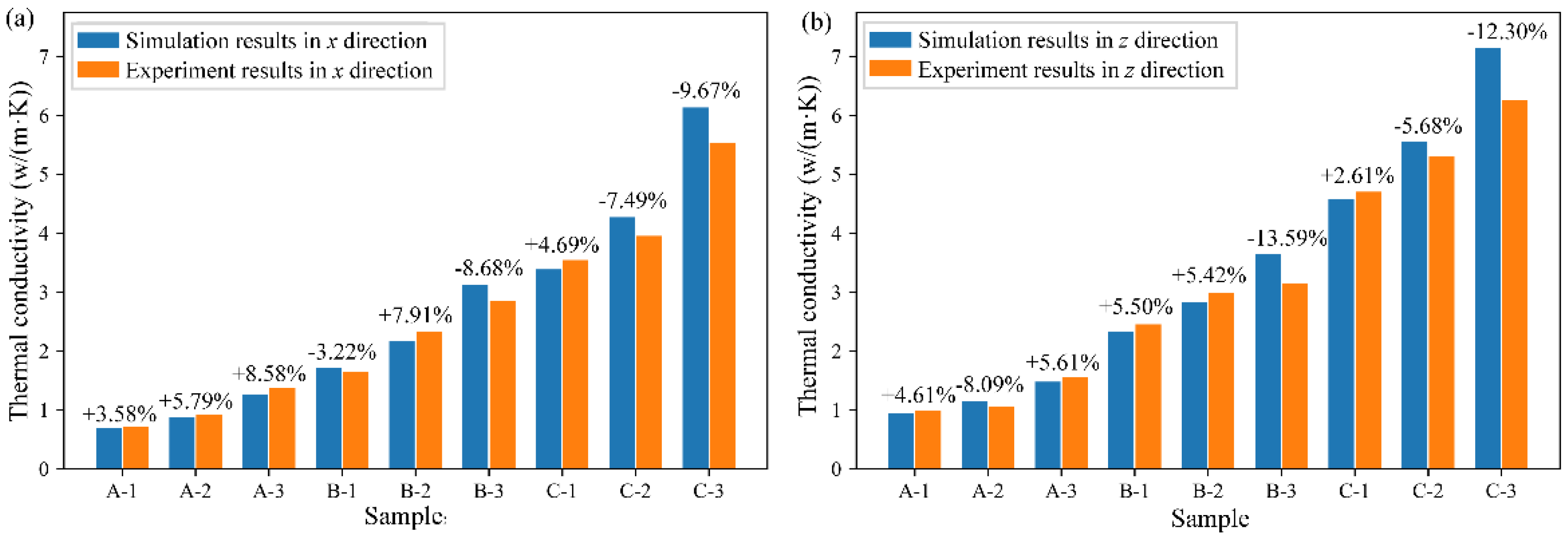
Figure 4 shows the comparison of the numerical-simulation results of different models of Litz winding with the experimental test results and the relative errors between the two. As depicted in Figure 4a, the numerical-simulation results of the thermal conductivity in the x direction of Litz winding were closer to the experimental results with a maximum relative error of 9.67%, while Figure 4b shows the comparative results in the z direction, which had a larger relative error of 13.59% than that in the x direction because the dimensions in the z direction were larger than those in the x direction; all errors were within acceptable limits. Therefore, the numerical-simulation model used in this paper is considered reasonable and can be used in the numerical simulation of the thermal conductivity of Litz winding for different operating conditions.

4. Results and Discussion

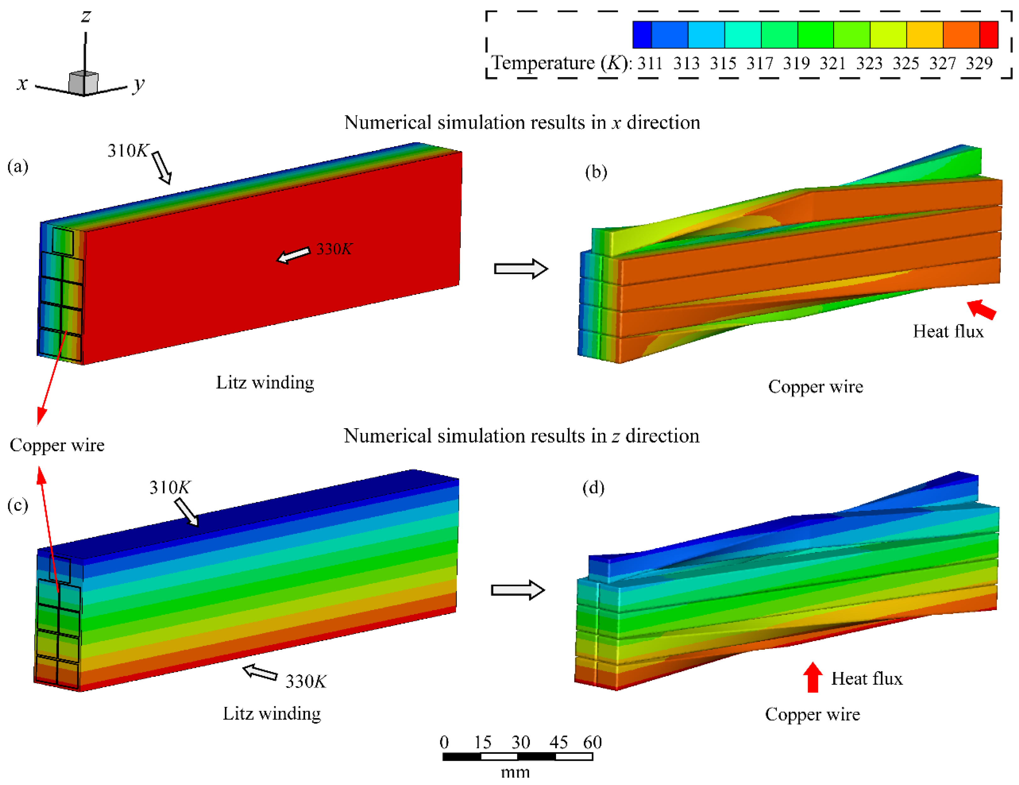
Numerical simulations of the thermal conductivity in the x and z directions were performed in ANSYS using steady-state thermal analysis for the transposed Litz winding 3D model. The bundle of wires inside the insulation has radial and axial thermal characteristics as well as local coordinates. As indicated in Figure 5a,c, in the numerical simulation of the thermal conductivity, the initial temperatures were given of the two corresponding surfaces along the x and z directions. Considering the stability of the material properties and the daily working temperature, the temperatures of the two corresponding surfaces were set to 310 K and 330 K , and the rest of the surfaces were set to be adiabatic surfaces without heat transfer. Under this boundary condition, the heat flow was smoothly conducted between the two faces. By observing the average heat flow on the cross-section in the simulation results, the equivalent thermal conductivity λ = q l Δ T A can be obtained, where λ ( W / m K ) is the thermal conductivity, q ( W ) is the heat flow rate, l ( m ) is the length along the heat flow direction, Δ T ( K ) is the temperature difference between the two corresponding surfaces perpendicular to the heat flow direction, and A ( m 2 ) is the cross-sectional area of the corresponding surface.
Since all Litz windings of different sizes have the same copper wire size and material properties, the thermal conductivity of Litz winding is only related to the filling rate and the material properties of the epoxy resin used. In order to facilitate the design of motor parameters, it is necessary to investigate the variation of Litz winding thermal conductivity with the change of filling rate and epoxy-resin material under different operating conditions using numerical-simulation models.

4.1. Effect of Filling Rate

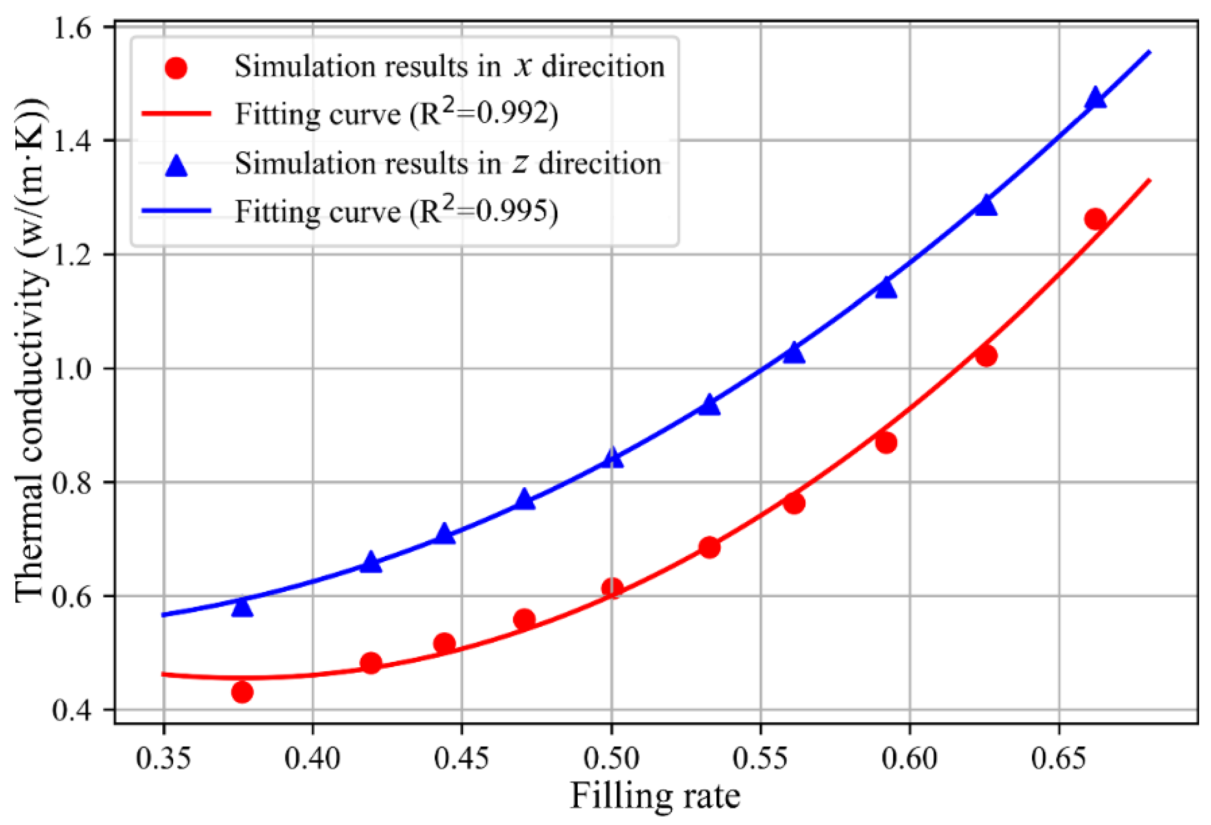
During the design process of motors, the dimensional parameters of Litz winding are often modified several times, and the modification of dimensions will directly change the filling rate of Litz winding, so it is of great importance to explore the relationship between the thermal conductivity of Litz winding and the filling rate. Ten Litz winding numerical models with different filling rates were selected to evaluate the effect of filling rate on thermal conductivity in the commonly used filling rate range of the motor. Epoxy resin 1 (0.2 W / m K ), which is commonly used in motor design, was used in all the numerical models. With the same copper wire specification, the dimension of epoxy resin was changed by changing the size of the numerical model, thus achieving a variation in the filling rate. The scattered data in Figure 6 show the numerical-simulation results of <span id = “zotero-drag”/> thermal conductivity in both x and z directions, and the thermal conductivity increased gradually with the increase in filling rate. However, since the discrete point data cannot continuously reflect the quantitative relationship between thermal conductivity and filling rate, the least square method was applied to fit the discrete data to obtain a convenient fitting equation that could reflect the thermal conductivity and filling rate, and which can be conveniently used in engineering design.
The least square method is for a given set of data ( u i , y i ) ( i = 0 , 1 , , m ), where u i is the filling rate and y i ( W / m K ) is the thermal conductivity. The function S * u in the function space Φ = span φ 0 , φ 1 , , φ n can be found such that th e error sum of squares (8) is minimized, and the equation S u is the fitting expression for the required solution S u = a 0 φ 0 ( u ) + a 1 φ 1 ( u ) + + a n φ n ( u )   ( n < m ) [28].
i = 0 m δ i 2 = i = 0 m S * u i y i 2 = min S u φ i = 0 m S u i y i 2
To make the S u more general, a weighted sum of squares (9) is fitted, where ω u 0 is the weight function within the fitted range:
i = 0 m δ i 2 = i = 0 m ω u i S u i y i 2
This translates into solving the multivariate Function (10) for the minimal points ( a 0 * , a 1 * , , a n * ) :
I a 0 , a 0 , , a 0 = i = 0 m ω u i j = 0 n a j φ j u i y i 2
From the necessary conditions for the extreme value of the multivariate function, it can be observed that:
I a k = 2 i = 0 m ω ( u i ) j = 0 n a j φ j ( u i ) y i φ k ( u i ) = 0 ( k = 0 , 1 , , n )
If we make ( φ j , φ k ) = i = 0 m ω ( u i ) φ j ( u i ) φ k ( x i ) , then we can get y , φ k = i = 0 m ω ( u i ) y i φ k ( u i ) d k   ( k = 0 , 1 , , n ) , i = 0 m ( φ k , φ j ) a j = d k   ( k = 0 , 1 , , n ) , from which we can obtain the expression of the fitting curve S u . Moreover, R 2 = S S T S S R = i = 1 n ( y i y ¯ ) 2 i = 1 n ( y ^ y ¯ ) 2 in goodness of fit is used to evaluate the fitting degree of the fitting curve to the observed values, where S S T is the total sum of squares, S S R is the regression sum of squares, y ¯ is the mean value of the data to be fitted, and y ^ is the fitted data. The closer R 2 is to 1, the better the fitting effect. In order to make the fitted curves as simple as possible with guaranteed accuracy and convenience for engineering calculations, S u = a 0 + a 1 u + a 2 u 2 was chosen for the fitting. The fitting curves are shown in Figure 6, in the range of filling rate from 0.35 to 0.7, the fitting curve of thermal conductivity in x direction and filling rate is expressed as S x u = 1.796 7.126 u + 9.468 u 2 , R 2 = 0.992 , and the fitting curve of thermal conductivity in z direction and filling rate is expressed as S z u = 1.072 3.728 u + 6.526 u 2 , R 2 = 0.995 .

4.2. Effect of Epoxy-Resin Type

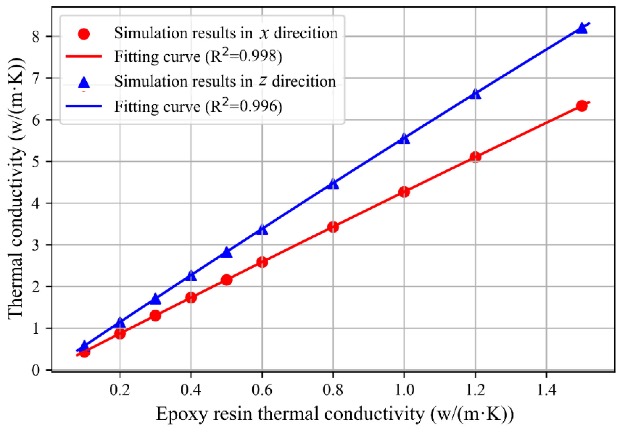
In addition to filling rate studies, it is often necessary to investigate the calculations for a wide range of epoxy-resin types. Similar to the investigation of the effect of filling rate, a numerical model of Litz winding with 10 different epoxy-resin types was selected to evaluate the effect of material property changes on thermal conductivity within the commonly used epoxy-resin material for electric motors. In order to control a single variable, each numerical model had the same filling rate and was simulated using a common size of 10.8 × 23.2   m m 2 (59.8% filling rate) in motor design, with the properties of each numerical model remaining the same except for the change in epoxy-resin material. The scatter plot in Figure 7 shows the results of the numerical simulation. As the thermal conductivity of epoxy resin increases, the thermal conductivity in both x and z directions increases, while the increase in the thermal conductivity of epoxy resin has limited incremental effect on the overall thermal conductivity of Litz winding due to the large proportion of copper wire in z direction. Therefore, the thermal conductivity growth rate of Litz winding in the z direction is much lower than that in the x direction. Similarly, the least square method is used for curve fitting of the discrete data points, and the fitting method is the same as in Section 4.1, which results in the fitting curve in Figure 7. When the thermal conductivity of epoxy resin is in the range of 0.1 W / m K to 1.5 W / m K , the fitting curve of thermal conductivity and filling rate in x direction is expressed as S x v = 4.365 v 0.095 v 2 , R 2 = 0.998 , where v is the thermal conductivity of epoxy resin, and the fitting curve of thermal conductivity and filling rate in z direction is expressed as S z v = 0.002 + 5.741 v 0.182 v 2 , R 2 = 0.996 , which can well describe the scattered data and complete the fitting.

4.3. Joint Effect of Filling Rate and Epoxy-Resin Type

After deriving the single variable function of thermal conductivity concerning filling rate and epoxy-resin thermal conductivity, the least square method and GA-BP neural network were used to explore the variation law of filling rate and epoxy-resin type on thermal conductivity to obtain a more extensive and refined quantification law.

4.3.1. Prediction with the Least Square Method

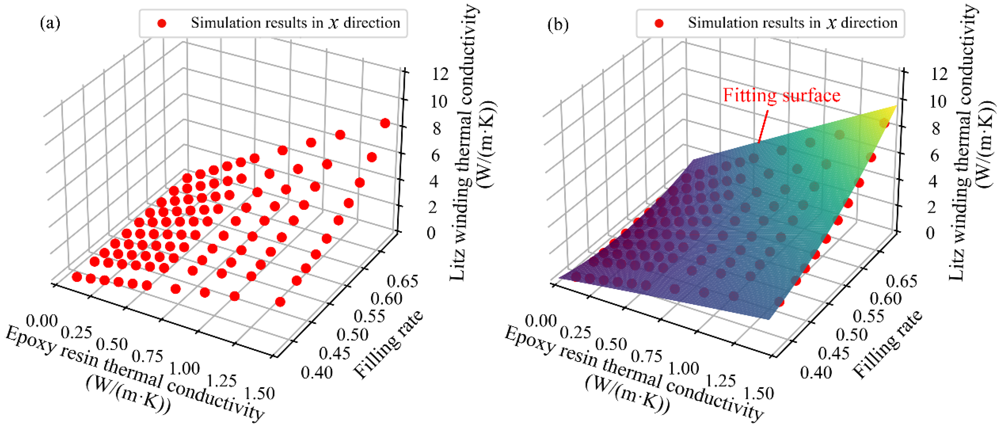
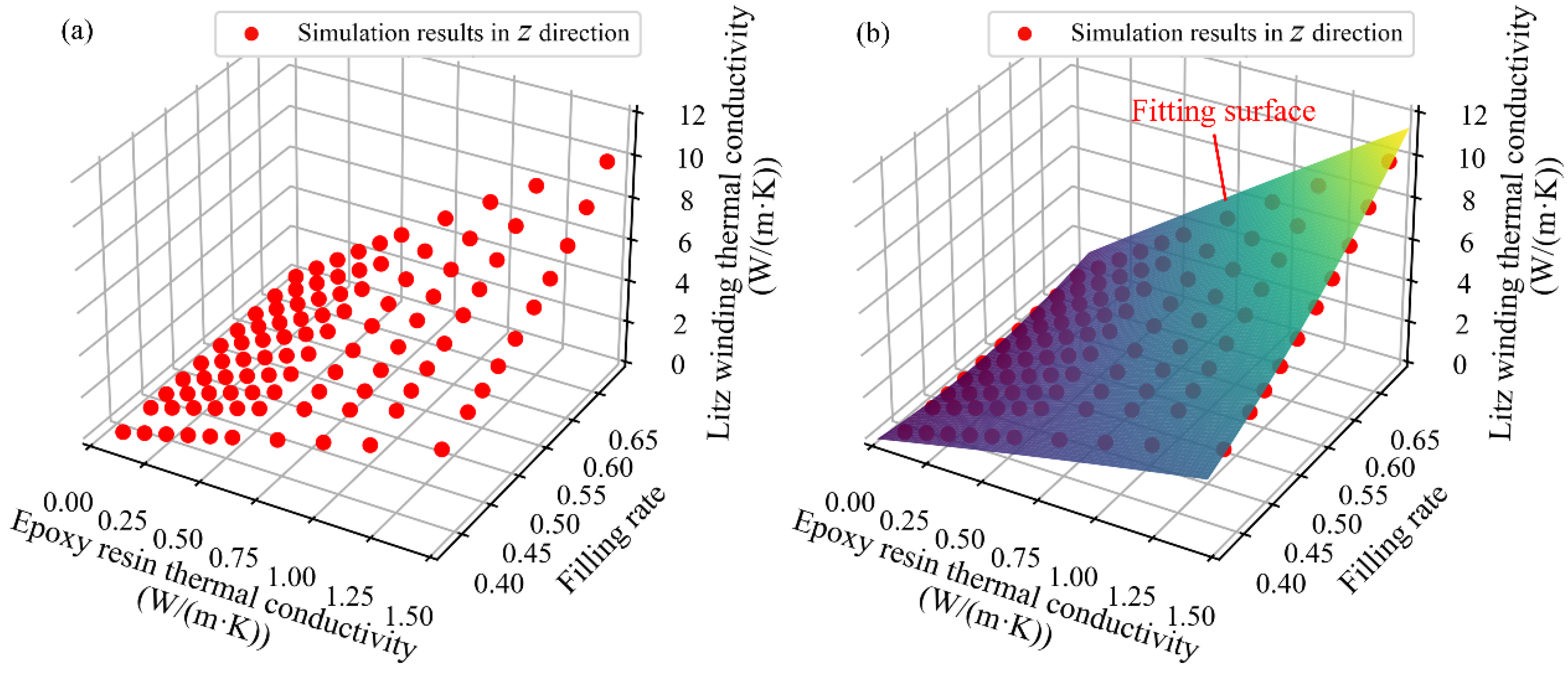
Figure 8 and Figure 9a show the variation of thermal conductivity in the x and z directions, respectively. Similar to the single variable law explored, the thermal conductivity of Litz winding gradually increases as the filling rate and the thermal conductivity of epoxy resin gradually rise. Because of the large proportion of copper wire in the z direction, the influence on the thermal conductivity in the z direction was greater than that in the x direction. For the three-dimensional discrete points where the filling rate and epoxy resin types interact together, the surface fitting can be carried out by referring to the least square method for the two-dimensional discrete points. For a set of measurements ( u i , v i ) ( i = 1 , 2 , , m ) of multivariate function y = f u , v , where u is the filling rate, v ( W / m K ) is the thermal conductivity of epoxy resin, and a set of weight data ω i > 0 ( i = 1 , 2 , , m ), the following Function (12) should be required:
S n ( u , v ) = k = 1 n a k φ k ( u , v )   ( n m )
Thus, Equation (13) should be minimized:
F a 0 , a 1 , , a n = i = 1 m ω i y i S n ( u i , v i ) 2
The equation is similar to the Function (9) in the two-dimensional discrete point fit, except that ( φ k , φ j ) = i = 1 m ω i φ k ( u i , v i ) φ i ( u i , v i ) . Therefore, the expression for the three-dimensional discrete point fitting surface can be obtained according to i = 0 m ( φ k , φ j ) a j = d k   ( k = 0 , 1 , , n ) . In order to make the fitting surface concise within the error control, S u = a 0 + a 1 u + a 2 v + a 3 u 2 + a 4 u v + a 5 v 2 is chosen to be fitted. The fitting surfaces obtained are shown in Figure 8 and Figure 9b. When the filling rate is in the range of 0.35 to 0.7 and the thermal conductivity is in the range of 0.1 W / m K to 1.5 W / m K , the fitting surface expression of the thermal conductivity in the x direction is S x u , v = 7.668 30.591 u 3.031 v 0.071 v 2 + 12.811 u v + 29.620 u 2 , R 2 = 0.988 . Simultaneously, the expression of the fitting curve of thermal conductivity versus filling rate in z direction is S z u , v = 5.107 20.560 u 2.604 v 0.135 v 2 + 14.171 u v + 20.079 u 2 , R 2 = 0.983 .
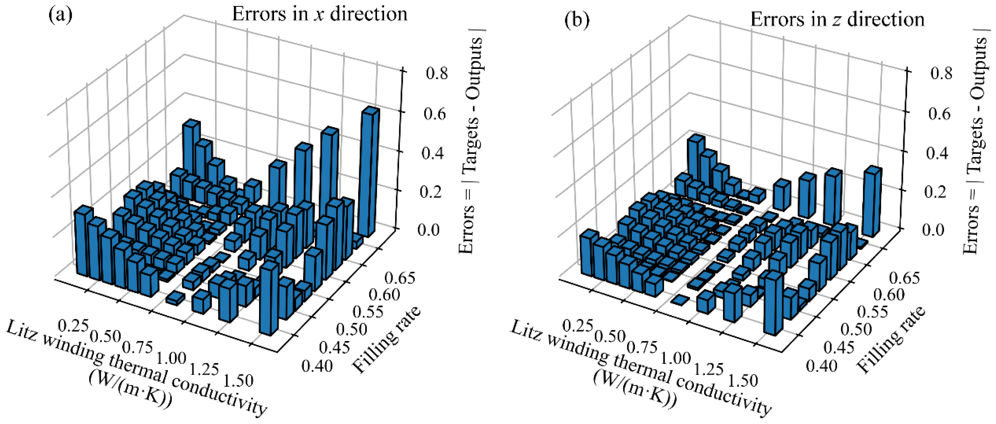
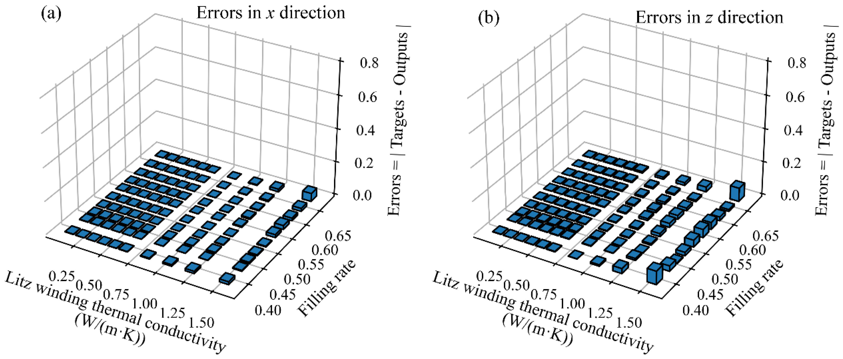
From the R 2 , it can be seen that the fitting surface has a descent fitting effect and can be used within the error tolerance in practical engineering, but as shown in the error distribution in Figure 10, when fitting the surface based on the least square method, the maximum error (abs (target−output)) in the x direction is 0.625, while the maximum error in the z direction is 0.326, implying that there are still large deviations in some data points when using this method for fitting. Therefore, although the least square method can be used as an empirical formula to guide engineering applications, in order to further optimize the results, facilitate the addition of new data in the future, and consider more complex and variable influencing factors, to improve the practicability and accuracy of the prediction method, the GA-BP neural network is also introduced for data prediction evaluation [29].

4.3.2. Prediction with GA-BP Neural Network

The BP neural network (back propagation neural network) consists of an input layer, an implicit layer, and an output layer [30]. Nodes between two adjacent layers are fully connected, and nodes within a layer are not attached. The forward transmission signal is transmitted from the input layer through each layer node to the output layer, and then the error between the output value and the true value is back propagated to each layer node, and the cycle continues to optimize the weights and thresholds until a satisfactory result is obtained [31,32,33]. However, the prediction accuracy of BP neural networks is greatly influenced by factors such as initial weights and thresholds, which are initialized randomly, making it difficult to obtain the best initial weights and thresholds. In addition, BP neural networks tend to fall into local optimality and cannot find the global optimal point, and the prediction ability depends on the representativeness of sample data. Consequently, it is usually necessary to introduce a genetic algorithm (GA) to optimize the initial weights and thresholds of BP neural networks [34]. A GA can improve the adaptability and optimization ability of various artificial systems by simulating biological genetic and variation and evolution in nature, and can fill the shortage of a BP neural network through the global search for optimization. The specific training process of the GA-BP neural network is depicted in Figure 11.
Filling rate and epoxy-resin thermal conductivity were used as input data and Litz winding thermal conductivity was adopted as output data. The first 70% of the input data was used as the training set and the latter 30% as the test set. After testing and exploring, the Levenberg–Marquardt backpropagation algorithm was used, the implied nodes were set to six layers, the crossover probability in the genetic algorithm was set to 0.4, and the population size was set to 80 for the training of the model. Figure 12 shows the distribution of errors in the x and z directions of the GA-BP neural network, and the errors on all data were significantly reduced compared to Figure 10. The maximum error of the GA-BP neural network in the x direction was only 0.081, R 2 = 0.9998 , and the error was reduced by 87.04%. In the z direction, it was 0.049, R 2 = 0.9999 , and the error was reduced by 84.97%. Compared with the least square method, it had a very significant combination effect and can provide reference for drawing more generalized conclusions in the future.

5. Conclusions

In this research, a numerical-simulation model of the thermal conductivity of Litz winding considering the transposition effect was developed, and the correctness of the numerical simulation was validated using the transient-plane-source method. The comparison results show that the maximum relative errors in the x and z directions were 9.67% and 13.69%, which were within the engineering allowable range and had a good simulation effect. In addition, using numerical models, the effects of filling rate and epoxy-resin type, and their combined effects, on thermal conductivity were explored independently. For the discrete data results, the least square method was used to analyze the data and fit the simpler and more convenient polynomial empirical functions. Furthermore, the maximum error between the prediction result and the target value in the x direction was reduced by 87.04% and R 2 increased from 0.988 to 0.9998 under GA-BP neural network, while the maximum prediction error in the z direction was reduced by 84.97% and R 2 raised from 0.983 to 0.9999. This result can provide a valuable contribution to the introduction of new variables and to high-precision estimation in the future design of the electrical motor.

Author Contributions

Conceptualization, Q.D.; Methodology, Q.D.; Data curation, X.F.; Writing—review & editing, X.F. All authors have read and agreed to the published version of the manuscript.

Funding

This research received no external funding.

Data Availability Statement

Not applicable.

Conflicts of Interest

The authors declare no conflict of interest.

References

  1. Kumar, D.; Gupta, R.A. A Comprehensive Review on BLDC Motor and Its Control Techniques. Int. J. Power Electron. 2021, 14, 292–335. [Google Scholar] [CrossRef]
  2. Zhao, J.; Zhang, B.; Fu, X.; Yan, S. Numerical Study on the Influence of Vortex Generator Arrangement on Heat Transfer Enhancement of Oil-Cooled Motor. Energies 2021, 14, 6870. [Google Scholar] [CrossRef]
  3. Sayed, E.; Abdalmagid, M.; Pietrini, G.; Sa’adeh, N.-M.; Callegaro, A.D.; Goldstein, C.; Emadi, A. Review of Electric Machines in More-/Hybrid-/Turbo-Electric Aircraft. IEEE Trans. Transp. Electrif. 2021, 7, 2976–3005. [Google Scholar] [CrossRef]
  4. Zhou, Y.; Dong, Q.; Niu, X.-J.; Xu, H.; Xiong, Q.; Su, H.; Zheng, J. A Pole Pair Segment of Oil-Cooling Air-Core Stator for a 2 MW Direct-Drive High Temperature Superconducting Wind Power Generator. J. Electr. Eng. Technol. 2021, 16, 3145–3155. [Google Scholar] [CrossRef]
  5. Inoue, S.; Akagi, H. A Bidirectional Isolated DC–DC Converter as a Core Circuit of the Next-Generation Medium-Voltage Power Conversion System. IEEE Trans. Power Electron. 2007, 22, 535–542. [Google Scholar] [CrossRef]
  6. Leibl, M.; Ortiz, G.; Kolar, J.W. Design and Experimental Analysis of a Medium-Frequency Transformer for Solid-State Transformer Applications. IEEE J. Emerg. Sel. Top. Power Electron. 2017, 5, 110–123. [Google Scholar] [CrossRef]
  7. Shen, W.; Wang, F.; Boroyevich, D.; Tipton IV, C.W. High-Density Nanocrystalline Core Transformer for High-Power High-Frequency Resonant Converter. IEEE Trans. Ind. Appl. 2008, 44, 213–222. [Google Scholar] [CrossRef]
  8. Sullivan, C.R. Optimal Choice for Number of Strands in a Litz-Wire Transformer Winding. IEEE Trans. Power Electron. 1999, 14, 283–291. [Google Scholar] [CrossRef]
  9. Carretero, C.; Acero, J.; Alonso, R. TM-TE Decomposition of Power Losses in Multi-Stranded Litz-Wires Used in Electronic Devices. Prog. Electromagn. Res. 2012, 123, 83–103. [Google Scholar] [CrossRef]
  10. Liu, X.; Gerada, D.; Xu, Z.; Corfield, M.; Gerada, C.; Yu, H. Effective Thermal Conductivity Calculation and Measurement of Litz Wire Based on the Porous Metal Materials Structure. IEEE Trans. Ind. Electron. 2020, 67, 2667–2677. [Google Scholar] [CrossRef]
  11. Sullivan, C.R.; Zhang, R.Y. Simplified Design Method for Litz Wire. In Proceedings of the 2014 IEEE Applied Power Electronics Conference and Exposition—APEC 2014, Long Beach, CA, USA, 25–29 March 2014; pp. 2667–2674. [Google Scholar]
  12. Jaritz, M.; Hillers, A.; Biela, J. General Analytical Model for the Thermal Resistance of Windings Made of Solid or Litz Wire. IEEE Trans. Power Electron. 2019, 34, 668–684. [Google Scholar] [CrossRef]
  13. Idoughi, L.; Mininger, X.; Bouillault, F.; Bernard, L.; Hoang, E. Thermal Model With Winding Homogenization and FIT Discretization for Stator Slot. IEEE Trans. Magn. 2011, 47, 4822–4826. [Google Scholar] [CrossRef]
  14. Yi, X.; Yang, T.; Xiao, J.; Miljkovic, N.; King, W.P.; Haran, K.S. Equivalent Thermal Conductivity Prediction of Form-Wound Windings with Litz Wire Including Transposition Effects. IEEE Trans. Ind. Appl. 2021, 57, 1440–1449. [Google Scholar] [CrossRef]
  15. Simpson, N.; Wrobel, R.; Mellor, P.H. Estimation of Equivalent Thermal Parameters of Impregnated Electrical Windings. IEEE Trans. Ind. Appl. 2013, 49, 2505–2515. [Google Scholar] [CrossRef]
  16. Wrobel, R.; Mellor, P.H. A General Cuboidal Element for Three-Dimensional Thermal Modelling. IEEE Trans. Magn. 2010, 46, 3197–3200. [Google Scholar] [CrossRef]
  17. Woodworth, A.A.; Jansen, R.; Duffy, K.; Nazhipour Author, P.; Shin, E.-S. Creating a Multifunctional Composite Stator Slot Material System to Enable High Power Density Electric Machines for Electrified Aircraft Applications. In Proceedings of the 2018 AIAA/IEEE Electric Aircraft Technologies Symposium (EATS), Cincinnati, OH, USA, 12–14 July 2018; pp. 1–8. [Google Scholar]
  18. Liu, H.P.; Hahne, J.J. High-Speed Compulsator Stator Thermal Management. IEEE Trans. Magn. 2003, 39, 357–361. [Google Scholar] [CrossRef]
  19. Huang, X.; Tan, Q.; Li, L.; Li, J.; Qian, Z. Winding Temperature Field Model Considering Void Ratio and Temperature Rise of a Permanent-Magnet Synchronous Motor with High Current Density. IEEE Trans. Ind. Electron. 2017, 64, 2168–2177. [Google Scholar] [CrossRef]
  20. Salinas López, G.; Expósito, A.D.; Muñoz-Antón, J.; Ramírez, J.Á.O.; López, R.P. Fast and Accurate Thermal Modeling of Magnetic Components by FEA-Based Homogenization. IEEE Trans. Power Electron. 2020, 35, 1830–1844. [Google Scholar] [CrossRef]
  21. Ke, J.; Wang, B.; Yang, Z. Application of GA and BP Neural Network in Heat Dissipation of Batteries. Mach. Des. Manuf. 2019, 11, 196–199. [Google Scholar] [CrossRef]
  22. Ivanova, A.; Migorski, S.; Wyczolkowski, R.; Ivanov, D. Numerical Identification of Temperature Dependent Thermal Conductivity Using Least Squares Method. Int. J. Numer. Methods Heat Fluid Flow 2019, 30, 3083–3099. [Google Scholar] [CrossRef]
  23. Jaritz, M.; Biela, J. Analytical Model for the Thermal Resistance of Windings Consisting of Solid or Litz Wire. In Proceedings of the 2013 15th European Conference on Power Electronics and Applications (EPE), Lille, France, 2–6 September 2013; pp. 1–10. [Google Scholar]
  24. Wrobel, R.; Ayat, S.; Baker, J.L. Analytical Methods for Estimating Equivalent Thermal Conductivity in Impregnated Electrical Windings Formed Using Litz Wire. In Proceedings of the 2017 IEEE International Electric Machines and Drives Conference (IEMDC), Miami, FL, USA, 21–24 May 2017; pp. 1–8. [Google Scholar]
  25. Chapman, B.L.W. Shielded gradients. And the general solution to the near field problem of electromagnet design. Magn. Reson. Mater. Biol. Phys. Med. 1974, 9, 146–151. [Google Scholar] [CrossRef] [PubMed]
  26. Gustafsson, S.E. Transient Plane Source Techniques for Thermal Conductivity and Thermal Diffusivity Measurements of Solid Materials. Rev. Sci. Instrum. 1991, 62, 797–804. [Google Scholar] [CrossRef]
  27. Dai, R.; Chandrasekaran, G.; Chen, J.; Jackson, C.; Liu, Y.; Nian, Q.; Kwon, B. Thermal Conductivity of Metal Coated Polymer Foam: Integrated Experimental and Modeling Study. Int. J. Therm. Sci. 2021, 169, 107045. [Google Scholar] [CrossRef]
  28. Kincaid, D.R.; Cheney, E.W. Numerical Analysis: Mathematics of Scientific Computing; American Mathematical Society: Providence, RI, USA, 2002. [Google Scholar]
  29. Huang, D.; Gong, R.-X.; Gong, S. Prediction of Wind Power by Chaos and BP Artificial Neural Networks Approach Based on Genetic Algorithm. J. Electr. Eng. Technol. 2015, 10, 41–46. [Google Scholar] [CrossRef]
  30. Wang, S.; Zhang, N.; Wu, L.; Wang, Y. Wind Speed Forecasting Based on the Hybrid Ensemble Empirical Mode Decomposition and GA-BP Neural Network Method. Renew. Energy 2016, 94, 629–636. [Google Scholar] [CrossRef]
  31. Papari, M.M.; Yousefi, F.; Moghadasi, J.; Karimi, H.; Campo, A. Modeling Thermal Conductivity Augmentation of Nanofluids Using Diffusion Neural Networks. Int. J. Therm. Sci. 2011, 50, 44–52. [Google Scholar] [CrossRef]
  32. Liu, H.-M.; Zhao, Y.-L.; Cheng, Y.-M.; Wu, J.; Al Shurafa, M.A.M.; Liu, C.; Lee, I.-K. A New Power Supply Strategy for High Power Rectifying Units in Electrolytic Copper Process. J. Electr. Eng. Technol. 2022, 17, 1143–1156. [Google Scholar] [CrossRef]
  33. Zhang, H.; Liu, Y. Adaptive RBF Neural Network Based on Sliding Mode Controller for Active Power Filter. Int. J. Power Electron. 2020, 11, 460–481. [Google Scholar] [CrossRef]
  34. Li, J.; Guo, B.; Shen, Y.; Li, D.; Huang, Y. A Modeling Approach for Energy Saving Based on GA-BP Neural Network. J. Electr. Eng. Technol. 2016, 11, 1289–1298. [Google Scholar] [CrossRef]
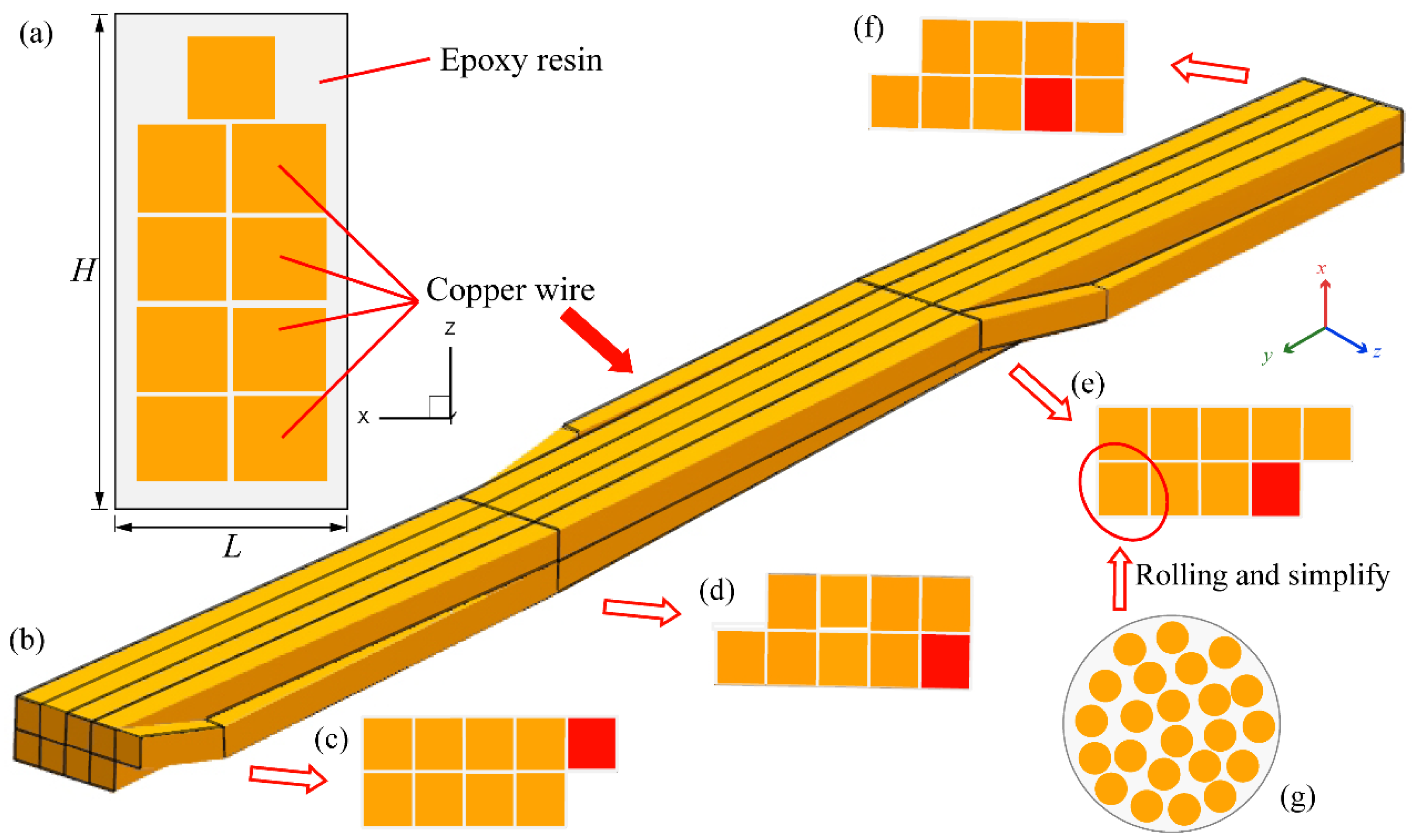
Figure 1. (a) Cross-section of Litz winding, (b) copper wire 3D model, (cf) cross-section of copper wire transposition structure, and (g) Litz-wire structure in single-strand copper wire.
Energies 16 07295 g001
Figure 2. (a,b) Representative grids in numerical simulation and (c) grid independence test results.
Energies 16 07295 g002
Figure 3. (a) Test instrument for the TPS method and (b) details of the test bench.
Energies 16 07295 g003
Figure 4. Validation of numerical results: (a) x direction and (b) z direction.
Energies 16 07295 g004
Figure 5. Numerical-simulation results: (a,b) x direction and (c,d) z direction.
Energies 16 07295 g005
Figure 6. Variation diagram of Litz winding thermal conductivity with filling rate.
Energies 16 07295 g006
Figure 7. Variation diagram of Litz winding thermal conductivity with epoxy-resin type.
Energies 16 07295 g007
Figure 8. (a) Scatter diagram and (b) fitting surface of Litz winding thermal conductivity in x direction with respect to filling rate and epoxy-resin type.
Energies 16 07295 g008
Figure 9. (a) Scatter diagram and (b) fitting surface of Litz winding thermal conductivity in z direction with respect to filling rate and epoxy-resin type.
Energies 16 07295 g009
Figure 10. Errors diagram using least square method: (a) in x direction and (b) in z direction.
Energies 16 07295 g010
Figure 11. GA-BP neural network training process diagram.
Energies 16 07295 g011
Figure 12. Errors diagram using GA-BP neural network: (a) in x direction and (b) in z direction.
Energies 16 07295 g012
Table 1. Materials and properties.
MaterialsThermal Conductivity
( W / m K )
MaterialsThermal Conductivity
( W / m K )
Copper wire387.6Epoxy resin 60.6
Epoxy resin 10.1Epoxy resin 70.8
Epoxy resin 20.2Epoxy resin 81.0
Epoxy resin 30.3Epoxy resin 91.2
Epoxy resin 40.4Epoxy resin 101.5
Epoxy resin 50.5
Table 2. Parameters of samples.
Serial NumberEpoxy-Resin Type Sample   Size   ( L H   m m 2 )Filling Rate (%)
A-1Epoxy resin 1
(0.2 W / m K )
11.6 × 24 53.8
A-2 10.8 × 23.2 59.8
A-3 10 × 22.4 66.2
B-1Epoxy resin 5
(0.5 W / m K )
11.6 × 24 53.8
B-2 10.8 × 23.2 59.8
B-3 10 × 22.4 66.2
C-1Epoxy resin 8
(1.0 W / m K )
11.6 × 24 53.8
C-2 10.8 × 23.2 59.8
C-3 10 × 22.4 66.2
Disclaimer/Publisher’s Note: The statements, opinions and data contained in all publications are solely those of the individual author(s) and contributor(s) and not of MDPI and/or the editor(s). MDPI and/or the editor(s) disclaim responsibility for any injury to people or property resulting from any ideas, methods, instructions or products referred to in the content.