Research on Q-Table Design for Maximum Power Point Tracking-Based Reinforcement Learning in PV Systems

Abstract

Photovoltaic (PV) power generation is considered to be a clean energy source. Solar modules suffer from nonlinear behavior, which makes the maximum power point tracking (MPPT) technique for efficient PV systems particularly important. Conventional MPPT techniques are easy to implement but require fine tuning of their fixed step size. Unlike conventional MPPT, the MPPT based on reinforcement learning (RL-MPPT) has the potential to self-learn to tune step size, which is more adaptable to changing environments. As one of the typical RL algorithms, the Q-learning algorithm can find the optimal control strategy through the learned experiences stored in a Q-table. Thus, as the cornerstone of this algorithm, the Q-table has a significant impact on control ability. In this paper, a novel Q-table of reinforcement learning is proposed to maximize tracking efficiency with improved Q-table update technology. The proposed method discards the traditional MPPT idea and makes full use of the inherent characteristics of the Q-learning algorithm such as its fast dynamic response and simple algorithm principle. By establishing six kinds of Q-tables based on the RL-MPPT method, the optimal discretized state of a photovoltaic system is found to make full use of the energy of the photovoltaic system and reduce power loss. Therefore, under the En50530 dynamic test standard, this work compares the simulation and experimental results and their tracking efficiency using six kinds of Q-table, individually.

1. Introduction

The PV power generation system is one of the most critical renewable energy systems since it has several advantages. The most significant of these are that they provide clean, accessible, and infinite resources [1]. PV arrays have different output power and voltage distributions at each irradiance/temperature level. This output power is nonlinear, and there is only one maximum power point under typical conditions. Many algorithms have been described in the literature for making PV modules at this point. Maximum power point tracking (MPPT) is the term for these algorithms [2,3]. Classic MPPT technologies are frequently used in practice due to their simplicity [4].

For example, the P&O method is simple and only involves using devices to detect photovoltaic current and voltage [5,6,7]. However, as the name suggests, this method constantly interferes with the operation of the converter by increasing/decreasing the fixed step size (FSS) to the photovoltaic source, causing oscillations in the output power. Another factor that has to be considered is that photovoltaic systems often exhibit a certain degree of uncertainty and volatility. For example, clouds and birds can cause significant changes in the photovoltaic P–V curve, at which point the FSS used leads to two main challenges: tracking speed and tracking accuracy. While a large FSS may increase the tracking speed, it may also lead to steady-state oscillations and increased power loss. In contrast, using a small FSS smoothes the oscillations but results in slow transients. These issues should be fully considered when designing a MPPT system for improved power tracking performance.

Many control strategies have been widely used in MPPT at the present stage, the most typical example being the variable step size (VSS) method [8,9,10]. In order to achieve a balance between speed and accuracy, the VSS method reduces the step size to minimize oscillations; a larger step size is adopted during transients to allow a fast speed. However, in order to adapt to changing weather conditions, the step size spin needs to be performed in real time. At the same time, the variable step size inevitably has a strong impact on the interharmonic current [11], and a smaller MPPT perturbation step size reduces the level of interharmonic emission but results in poorer tracking performance of the MPPT algorithm.

Therefore, many artificial intelligence (AI) [12]-based methods are widely applied to generate VSS optimal solutions, such as neural network-based control [13], repetitive control [14], fuzzy logic control [15], model predictive control [16], and particle swarm optimization control [17]. The above methods are suitable for theoretical modeling or cases where the subset of parameters is unknown. However, there are certain drawbacks in the application process of these control strategies. For example, neural network control requires a large amount of datasets for offline training, repetitive control cannot adapt to the rapidly changing situation of photovoltaics due to its slow dynamic response, fuzzy logic control provides high-speed tracking and zero oscillation at the cost of computational complexity, model predictive control requires high accuracy for system parameters, and particle swarm optimization control easily falls into local extreme points when the P–V curve of multiple photovoltaic arrays has multiple local extreme points, resulting in incorrect results. Due to its inherent characteristics such as fast dynamic response and simple algorithmic principle, the Q-learning algorithm has been widely studied in recent years.

As a reinforcement learning algorithm [18], the Q-learning algorithm does not require trained models or previous knowledge during implementation. The core of the Q-learning algorithm is the control strategy, because it suffices to decide the control actions by itself. The general strategy is to set up a searchable Q-table [19], which contains the state space and action space. The state space contains all the operational states of the potential system, and the action space contains all potential control actions. In recent years, many people have studied the Q-table. In [20], the clock arrival time of each register is updated using the Q-table to maximize the designed clock arrival distribution to reduce the peak current. In [21], a learning-based dual Q power management method is proposed to extend the operating frequency to improve the embedded battery life and provide a sustainable operating energy. It overturns the traditional Dynamic Voltage and Frequency Scaling (DVFS) method. In [22], a dynamic weight coefficient based on Q-learning for Dynamic Window Approach (DQDWA) is proposed. The robot state, environmental conditions, and weight coefficients are used as the Q-table for learning to better adapt to different environmental conditions.

However, little research has been performed on how to set the Q-table, which is crucial to the tracking performance in MPPT. This paper proposes a reinforcement learning Q-table design scheme for MPPT control, aiming to maximize the tracking efficiency through improved Q-table update techniques. Six kinds of Q-tables based on the RL-MPPT method are established to find the optimal discrete value state of the photovoltaic system, make full use of the energy of the photovoltaic system, and reduce the power loss. The En50530 dynamic test procedure is used to simulate the real environment and evaluate the tracking performance fairly [23], while switching between static and dynamic conditions.

The remainder of this paper is structured as follows. Section 2 describes the basic principles of the RL method. In Section 3, the tracking performance of three discrete values is evaluated through testing. Section 4 summarizes the paper.

2. Method

2.1. Fundamentals of RL

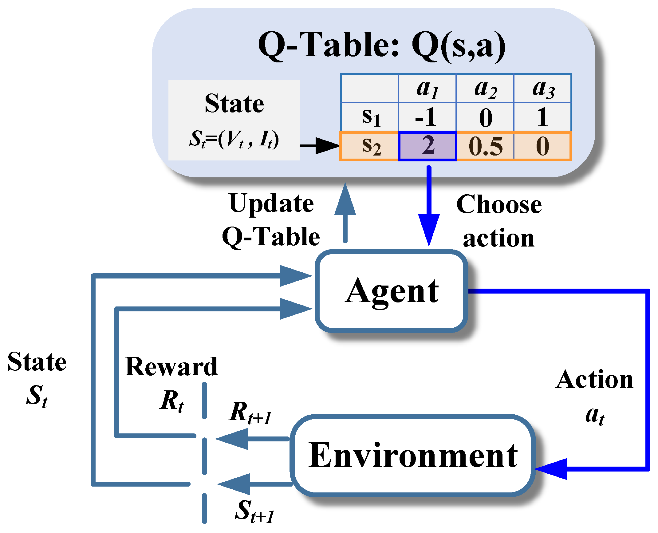
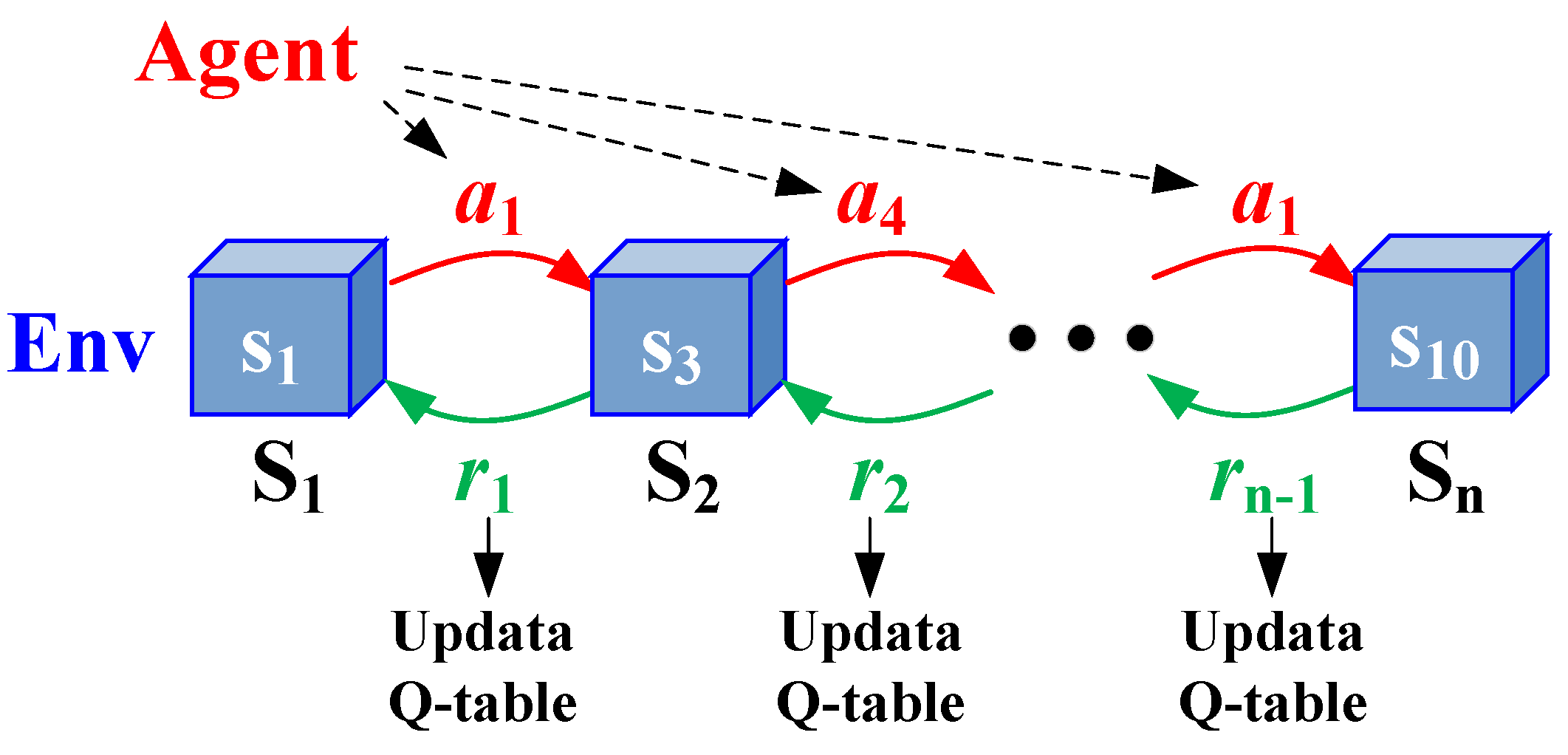
Reinforcement learning is an approach to machine learning that finds optimal behavioral strategies to maximize cumulative rewards by allowing an intelligent body to continuously try and learn in an environment. The basic concepts of reinforcement learning include intelligences, environments, states, actions, rewards, strategies, and goals.

RL is a approach of learning that maps situations to actions to maximize return. Figure 1 and Figure 2 indicate that the RL methods are typically used in frameworks that include agents and environments. Instead of being told which actions to take, the agent is a learner which uses the interaction process to find which action yields the max reward. The things with which it interacts are called the environment. A Markov Decision Process (MDP) is when an agent and an environment talk to each other. The agent sees what is happening in the environment, and then performs some action to change it. If the agent and the environment have only a few choices, then there is always a best way for the agent to act.

Many RL methods have been proposed. Q-learning, as one of the popular RL methods, is used as the value function in this paper. The Q is defined by

$$\begin{array}{c}\hfill Q_{t+1}\left(s_{t,}{a}_t\right)=\eta \left[r_{t+1}+\gamma \underset{a\in A}{max}{Q}_{t+1}\left(s_{t+1,}{a}_t\right)-Q_t\left(s_{t,}{a}_t\right)\right]\\ \hfill +Q_t\left(s_{t,}{a}_t\right)\end{array}$$

(1)

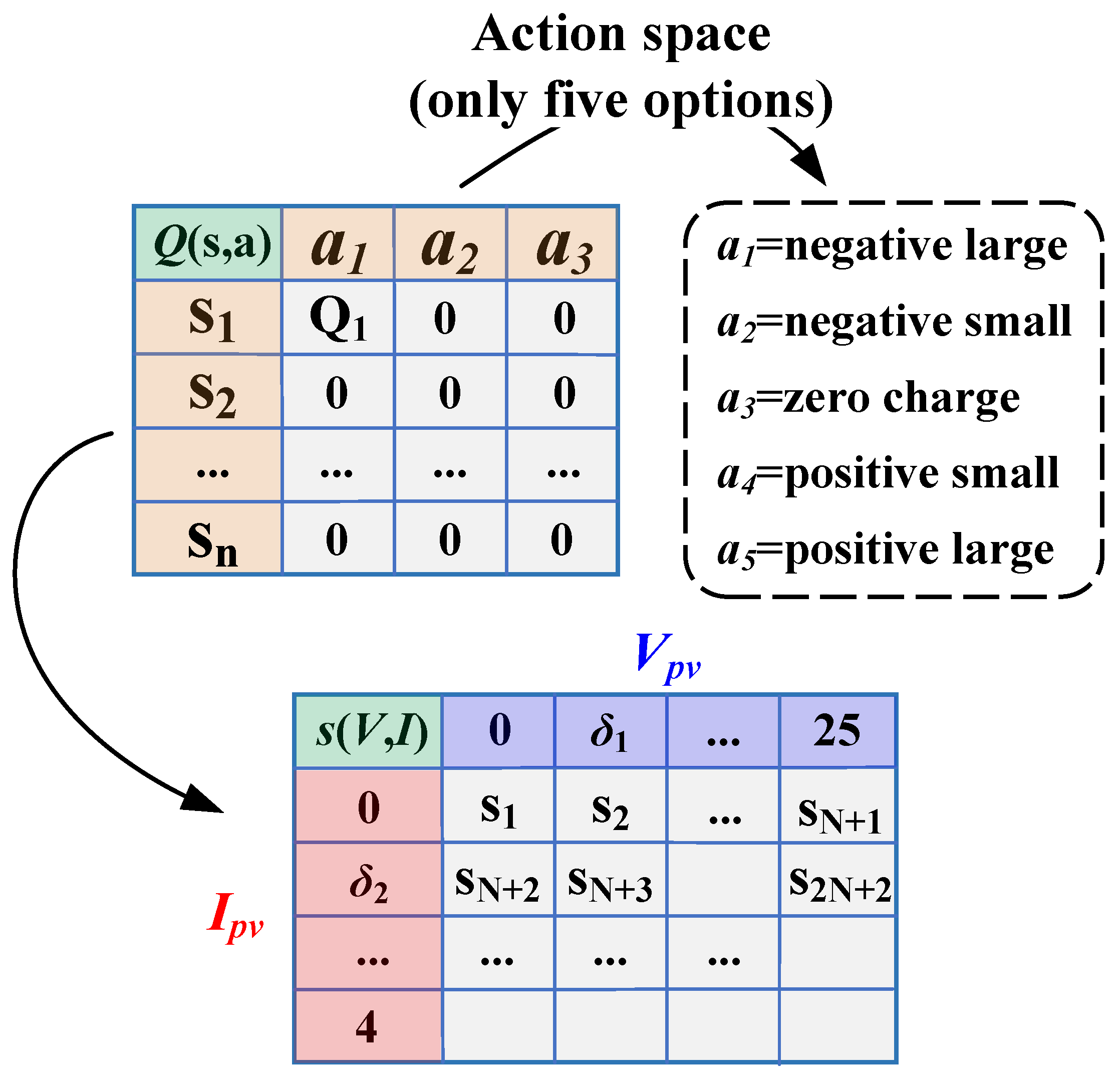
where $\eta \in \left(0,1\right]$ and $\gamma \in \left[0,1\right)$ represent learning rate and discount factor, respectively. s, a, and r are state, action, and reward, respectively. Meanwhile, there exists a Q-table that records the Q-value of each state–action space to provide a basis for formulating the optimal policy, as shown in Figure 3.

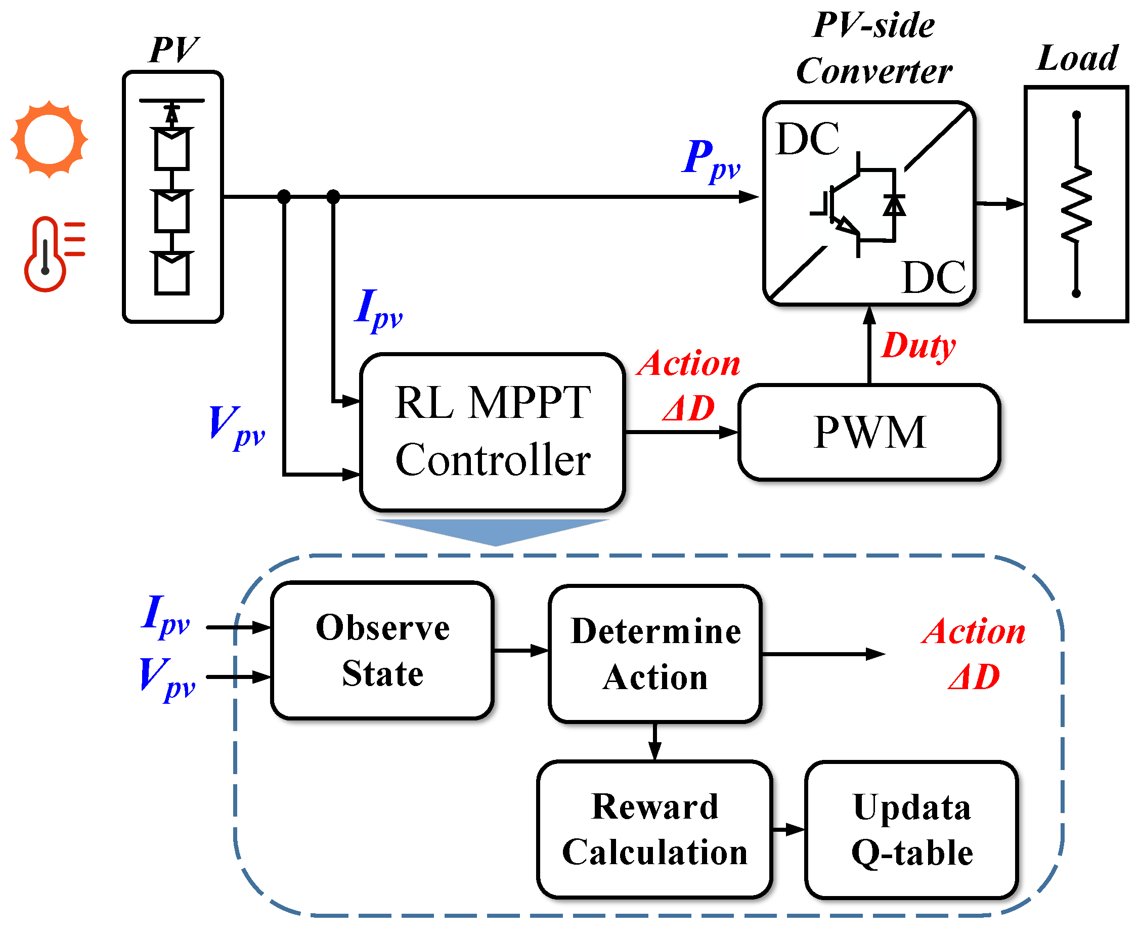
The power supply circuit and its layout are shown in Figure 4. The RL-MPPT controller, the agent, perceives the state $s\in S$ by the $V_{pv}$ and $I_{pv}$; the operating point on the I–V curve is then determined. Further, the variance in the duty cycle $\Delta D$ is output by the agent (i.e., the controller), which is the action $a\in A$. The control signal outputs a pulse with the corresponding D through the PWM, which acts as a switch to drive the boost converter. Finally, the reward r for the previous action shall be calculated.

2.1.1. Q-Table Setup

The Q-table approach in reinforcement learning is a value-based, model-free, off-track strategy reinforcement learning algorithm. Its purpose is to guide an intelligent body to choose the optimal action in each state by learning a Q-function. The Q-function represents the expectation of the long-term cumulative reward that can be obtained after executing action a in state. The Q-function is a function of the value of the action. Q-tables can be similar to a memorized database, which can store the experience and store the reward from each step of iteration between the agent and the environment. The main dimensions in the Q-table can be created by the state and action. The original Q-value is set to zero at the beginning of the Q-table. The reward can be calculated based on the state and action in each iteration. The Q-table is then updated in each iteration to store the latest rewards. Q-learning generally consists of two parts: the process of exploration and the process of utilization. During exploration, the agent randomly chooses an action to explore the state–action space and is rewarded accordingly. The Q-table is then structured and gradually becomes complete in this process of exploration. During exploitation, the agent chooses the action with the highest Q-value to execute the optimal program. In the Q-learning algorithm, four main items should be properly defined, i.e., state space, action space, reward function, and symbols.

2.1.2. State

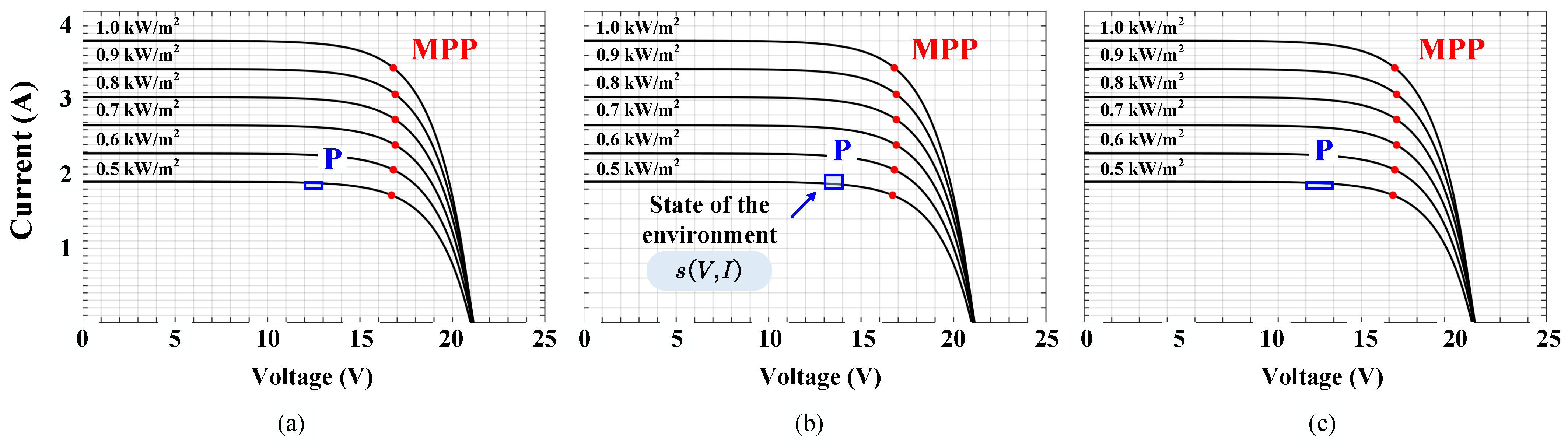
A Q-table in reinforcement learning is a table for storing state–action correspondences of value functions, which can be used to implement value-based reinforcement learning algorithms such as Q-learning. A state space is the set of all possible states, e.g., in a maze game, each grid is a state. In reinforcement learning, the size and complexity of the state space affects the feasibility and efficiency of Q-tables. If the state space is discrete and finite, the Q-table can be represented by a two-dimensional array, where each row corresponds to a state, each column corresponds to an action, and each element stores the value of that state–action pair. In this case, the Q-table can be continuously updated to approximate the optimal value function. Only enough descriptive information is available to define the state space, rather than utilize the agent to make control decisions. However, the large amount of information may result in a complex state space, which inevitably increases the difficulty. In contrast, too little information may result in a weak ability to discriminate between types of states, which will result in a less effective decision-making ability. Throughout this paper, the location of the run point can be described by the measurable $V_{pv}$ and $I_{pv}$. The state space is represented as

$$S=\left\{\left(V_{pv},I_{pv}\right)\right\}$$

(2)

The voltage variable $V_{pv}$ is discrete from 0 to 25 V and the current variable $I_{pv}$ is discrete from 0 to 4 A. As shown in Figure 5, three discrete values are set in this paper; in this way the tracking performance of different state spaces is compared.

2.1.3. Action

The action space is the set of all possible actions that can be taken by an intelligent body in reinforcement learning. The size and complexity of the action space affects the design and effectiveness of the reinforcement learning algorithm. Action spaces can be categorized into two types: discrete and continuous. The advantage of a discrete action space is that it is easy to represent and compute. However, the disadvantage is that it may not be able to cover all the action choices or lead to an action space that is too large and difficult to explore. The advantage of continuous action spaces is that they allow for more precise control of an intelligent agent’s behavior. However, the disadvantage is that it is difficult to represent and optimize with tables or discrete functions, and it needs to be solved using methods such as function approximation or policy gradient. In this paper, for the control of MPPT the discrete action space should be realized using the control duty cycle.

This study specifies a discrete, finite action space for applying Q-learning to MPPT [24]. The action space needs to follow rules as (a) both positive and negative changes must be included in the action space; (b) the action needs to be given enough small resolution to attain optimum power; (c) in order to eliminate oscillations between states, a zero-charge action must be provided. For MPPT, the state is determined after measuring $V_{pv}$ and $I_{pv}$. The movement of the running point can then be determined based on the actions chosen by the exploration strategy and the optimal strategy. Here, the action space is described in terms of five duty cycle $\Delta D$ steps (i.e., five actions) and is defined as

$$A=\left\{a|a_1,a_2,a_3,a_4,a_5\right\}$$

(3)

where the values of $a_1$ and $a_5$ indicate large positive and negative changes. Further, smaller positive and negative changes are indicated by $a_2$ and $a_4$. Finally, no change in duty cycle is denoted by $a_3$. To examine the tracking performance of several Q-tables, this study built up two separate action spaces, as shown in

Table 1. Two different type action spaces.

	${\mathit{a}}_1$	${\mathit{a}}_2$	${\mathit{a}}_3$	${\mathit{a}}_4$	${\mathit{a}}_5$
Type 1	−0.02	−0.005	0	0.005	0.02
Type 2	−0.01	−0.005	0	0.005	0.01

.

2.1.4. Reward

The effect of the interaction is measured by the reward function returning a scalar value [25]. The reward is a response from the “environment” as a result of action a for a state transition from s to $s^{\prime }$.

Usually, the previous action is evaluated by it. And the agent is taught how to choose the action. The reward function is expressed by

$$r_{t+1}=\left\{\begin{array}{c}{w}_p\frac{\Delta P_{t+1}}{\Delta t},if\frac{\Delta P_{t+1}}{\Delta t}<-\delta \\ \\ w_n\frac{\Delta P_{t+1}}{\Delta t},if\frac{\Delta P_{t+1}}{\Delta t}>\delta \\ \\ 0,if\left|\frac{\Delta P_{t+1}}{\Delta t}\right|<\delta \end{array}\right.$$

(4)

$$\Delta P_{t+1}=P_{t+1}-P_t$$

(5)

where the current power is $P_{t+1}$ and the previous power is $P_t$. Setting $\delta$ achieves the elimination of incorrect agent actions affected by measurement noise. The chosen action will result in a power rise indicated by a positive reward and vice versa. The reward weights can be set to $w_p=1.5$, $w_n=1$, thus reducing the convergence time.

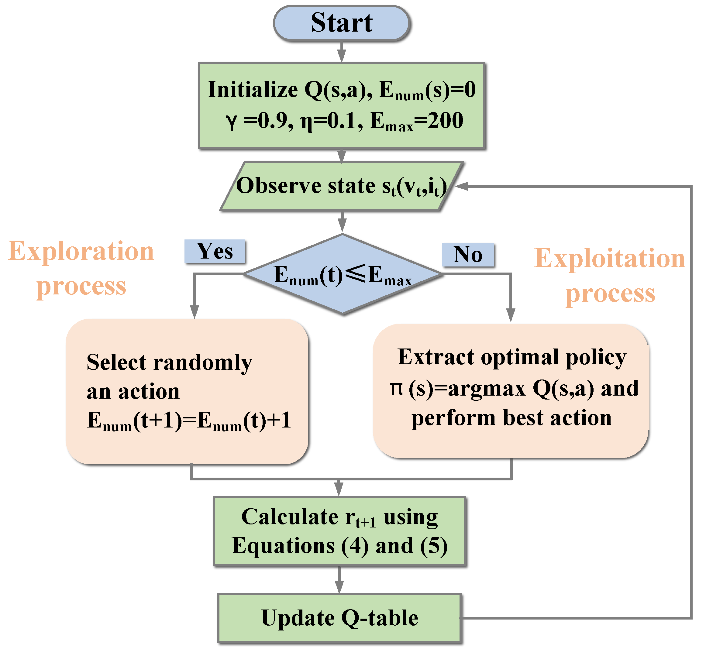
The RL method flowchart is shown in Figure 6. Firstly, the discount factor $\gamma$, the maximum number of exploring $E_{max}$, and the Q-table $Q_{(s,a)}$ are initialized. The voltage and current of PV system are measured to perceive the corresponding state in one iteration. Whether the current iteration is an exploration process or an exploitation process can be determined. During exploration, the next action will be randomly selected from space A. The action with the maximum Q-value will be selected in the exploitation process in the Q-table. According to (4), the reward $r_{t+1}$ of the previous action will be calculated and then stored in the Q-table.

2.2. The RL Algorithm

In this paper, Q-learning is applied to MPPT control. Through the interaction with the environment, the intelligent body can learn the optimal policy by feeding back the rewards, and then improve the performance of maximum power point tracking. In general, Q-learning is divided into two parts: the exploration process and exploitation process. In the exploration process, the intelligent body randomly selects an action to explore the environment and obtains the corresponding reward. The agent should explore the environment as much as possible and accumulate enough state–action space exploration experiences to accumulate experience. However, the algorithm cannot keep exploring; the algorithm needs to enter the exploitation phase to apply the previously accumulated experience and execute the optimal action through the previously acquired experience.

In an RL environment, the agent uses a trial-and-error process to learn the optimal policy as it interacts with the environment, rather than utilizing the model’s a priori knowledge [26]. The main meaning of the term “learning” is that the agent translates its experience that it gains from the interaction into knowledge. Depending on the objective optimal policy or optimal value function, RL algorithms can be categorized to two groups: the first are value-based approaches and the second are policy-based approaches. Q-learning is an approach that is value-based and model-free. For an MPPT algorithm, the state information that is measurable is accepted as an input signal, and the change in duty cycle is considered as an output signal. When initialization is complete, the current state $s_t$ is firstly observed by the algorithm. With the exploration count $E_{num}$, the algorithm can determine whether the current iteration is an exploitation process or an exploration process. During exploration, this algorithm will choose the next action a randomly. However, convergence to the optimal Q-function is still ensured under the assumption that the state–action set is finite, discrete, and has an infinite number of visits. The algorithm will switch to the exploitation process when the exploration process is over (i.e., the $E_{num}$ is equal to the threshold $E_{max}$). In this process, the action with the largest Q-value in the Q-table will be chosen by the agent (i.e., it extracts the optimal policy). For both an exploration process or an exploitation process, the award that corresponds to the previous operation will be counted and then updated in the Q-table.

In order to achieve the optimal action selection strategy, traditional RL methods require a large number of exploratory iterations. However, it is time-consuming and infeasible to explore a huge state–action space. In addition, if the exploration process ends, traditional RL methods cannot gain experience beyond optimal decision-making through interaction with the environment. Once the solar irradiation changes rapidly, traditional RL methods must return to the exploration process and re-accumulate the exploration experience to update the optimal action strategy, which may lead to tracking failure.

2.3. Comparison Results with Other Methods

For a clear comparison with other methods. We have added results comparing the P&O method with a fixed step size, the P&O method with a variable step size, and the proposed Q-table method under the En50530 dynamic test program.

Although the Q-table RL method is compared with the fixed-step as well as variable-step MPPT methods. However, it can be seen from Figure 7, Figure 8 and Figure 9 that the RL method becomes more and more accurate after continuous exploration and iteration. In addition, when the PV module has problems such as corrosion and aging, the MPPT points will be shifted, and the learning iteration RL method can avoid this problem.

3. Results

The simulation model was implemented using Matlab/Simulink software.

Table 2. Main product parameters of the PV module MSX-60W.

Parameter	Symbol	Value
Maximum power	$P_{mpp}$	60 W
Current at MPP	$I_{mpp}$	3.5 A
Voltage at MPP	$V_{mpp}$	17.1 V
Short-circuit current	$I_{sc}$	3.8 A
Open-circuit voltage	$V_{oc}$	21.1 V
Temperature coefficient of $I_{sc}$	$K_i$	0.065%/${}^{°}$C
Temperature coefficient of $V_{oc}$	$K_v$	−80 mV/${}^{°}$C

presents the crucial data of the solar module. It should be noted that the is set to 0.1 s.

In order to validate the effectiveness of the proposed Q-table method, the experimental setup is physically shown in Figure 10 using hardware-in-the-loop (HIL). The DSP used is the TMS320F28335 model manufactured by Texas Instruments. The DSP can sample the voltage and current of the MT6016 through an analog-to-digital converter (ADC), and then generate PWM control signals through the controller area network (CAN). The hardware configuration is simulated by a transient simulation software developed by StarSim, Inc. (Shanghai, China). The HIL system provides PV voltage and current measurements and obtains PWM control signals through an interface.

The parameters of the experimental tests are the same as those of the simulations. The RL-MPPT algorithm is applied and implemented by Simulink Matlab 2018b functions through the Embedded Encoder Support Package for the Texas Instruments C2000 processor, without the need for any additional libraries. The parameters of the experimental test circuit are the same as in the simulation. The sampling time (frequency) for the MPPT controller is taken as 0.1 s.

3.1. En50530 Dynamic Test Condition

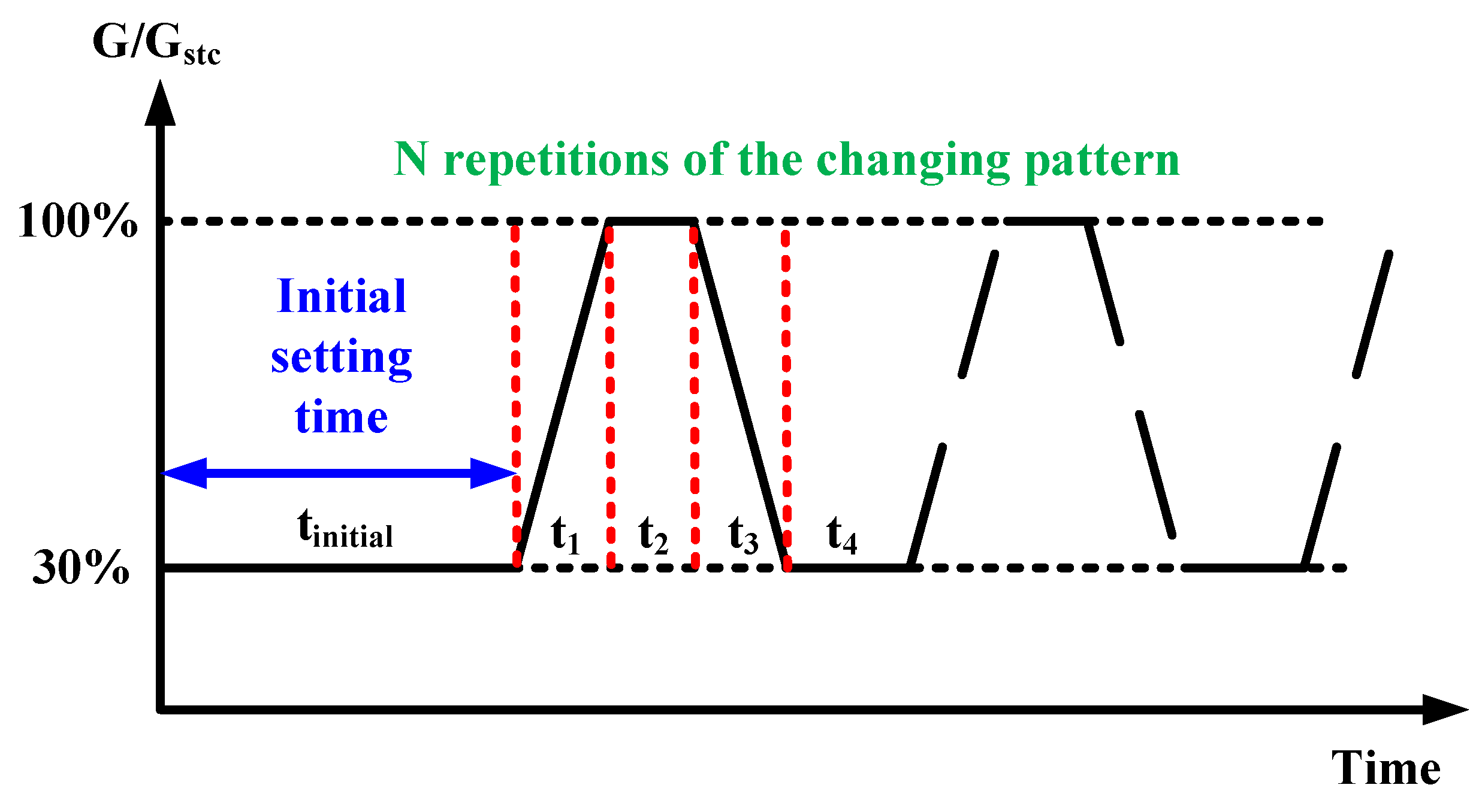
The test conditions closely simulate the operational environment of real photovoltaic systems by considering both and. Moreover, the test is particularly handy for indoor use. This paper focuses on the most difficult aspect of the test procedure [2]. As depicted in Figure 11, this specific part exhibits a gradient variation in irradiance ranging from 300 W/m${}^2$ to 1000 W/m${}^2$ at a rate of 100 W/m. The dynamic efficiency can be mathematically expressed as follows,

$${\eta }_d=\frac{{\sum }_i{P}_{pv}\times \Delta T_i}{{\sum }_j{P}_{max}\times \Delta T_j}$$

(6)

where $P_{max}$ and $\Delta T_j$ represent theoretical power and corresponding time, while $P_{pv}$ and $\Delta T_i$ denote real power and corresponding time.

3.2. Simulation Result

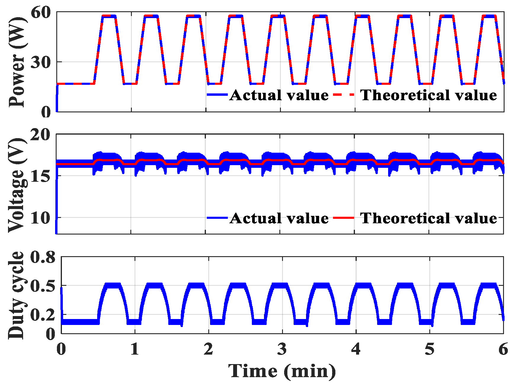
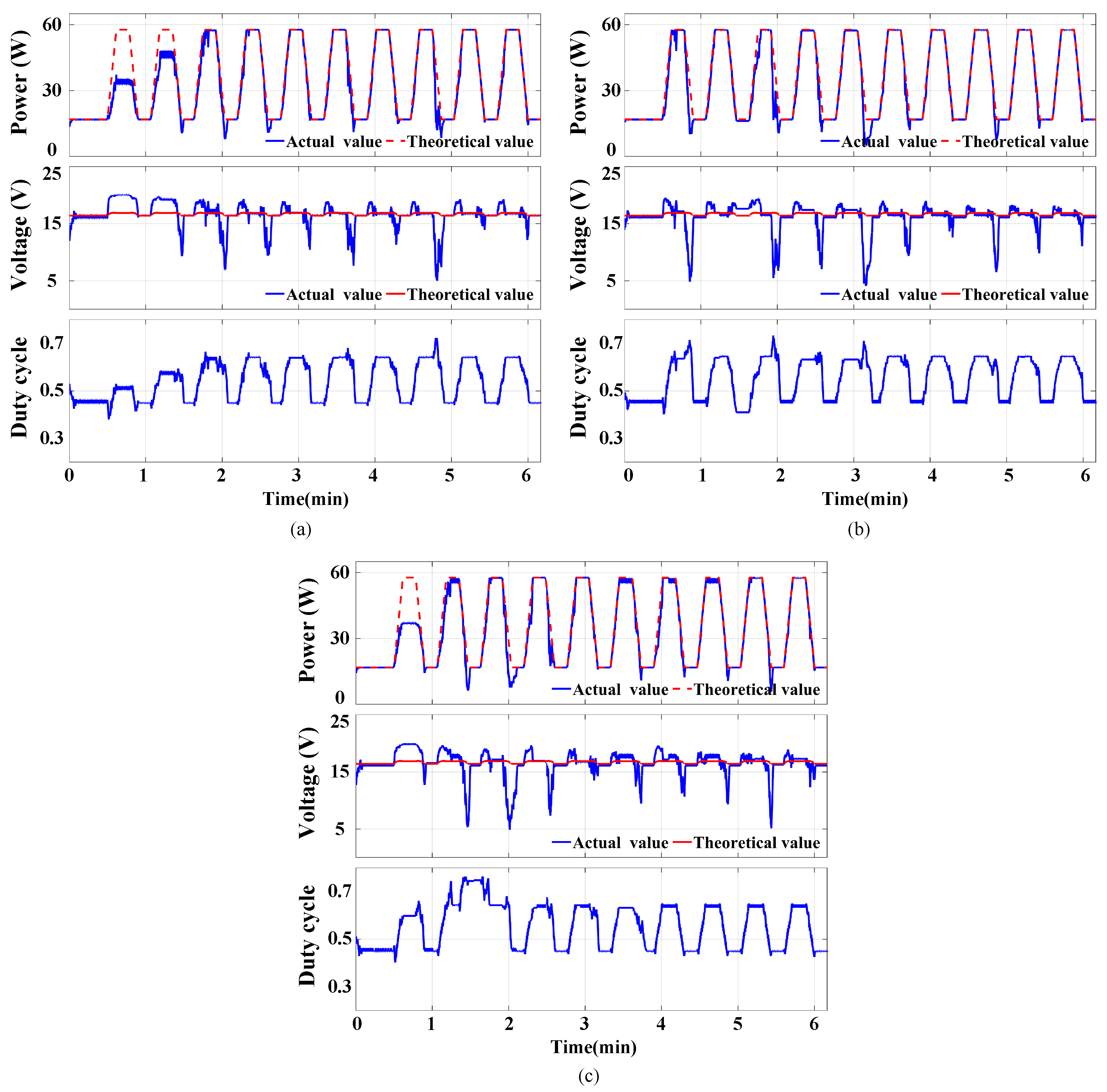
The contrast of power, voltage, and duty cycle is illustrated among Figure 12 and Figure 13, with the red dashed lines representing theoretical values. Among the three types of state space, the second type exhibits the highest at 95.55%, surpassing that of the first type (92.32%) and the third type (93.44%).

It is worth noting that a smaller discretization value results in more convergence time, leading to power loss. Furthermore, once the Q-table has converged, employing a reasonable discretization value contributes to more precise tracing accuracy compared to using a larger one. Therefore, it is recommended to utilize a moderate discretization value for the long-term operation of the RL-MPPT method. Additionally, regardless of the chosen discretization value, the RL-MPPT method will generate a bigger voltage deviation during irradiance decrease; however, this issue can be mitigated by adopting a smaller discretization value. Conversely, utilizing a huge discretization value may bring about significant vibration in the stable state as it fails to precisely locate and maintain operation at the MPP.

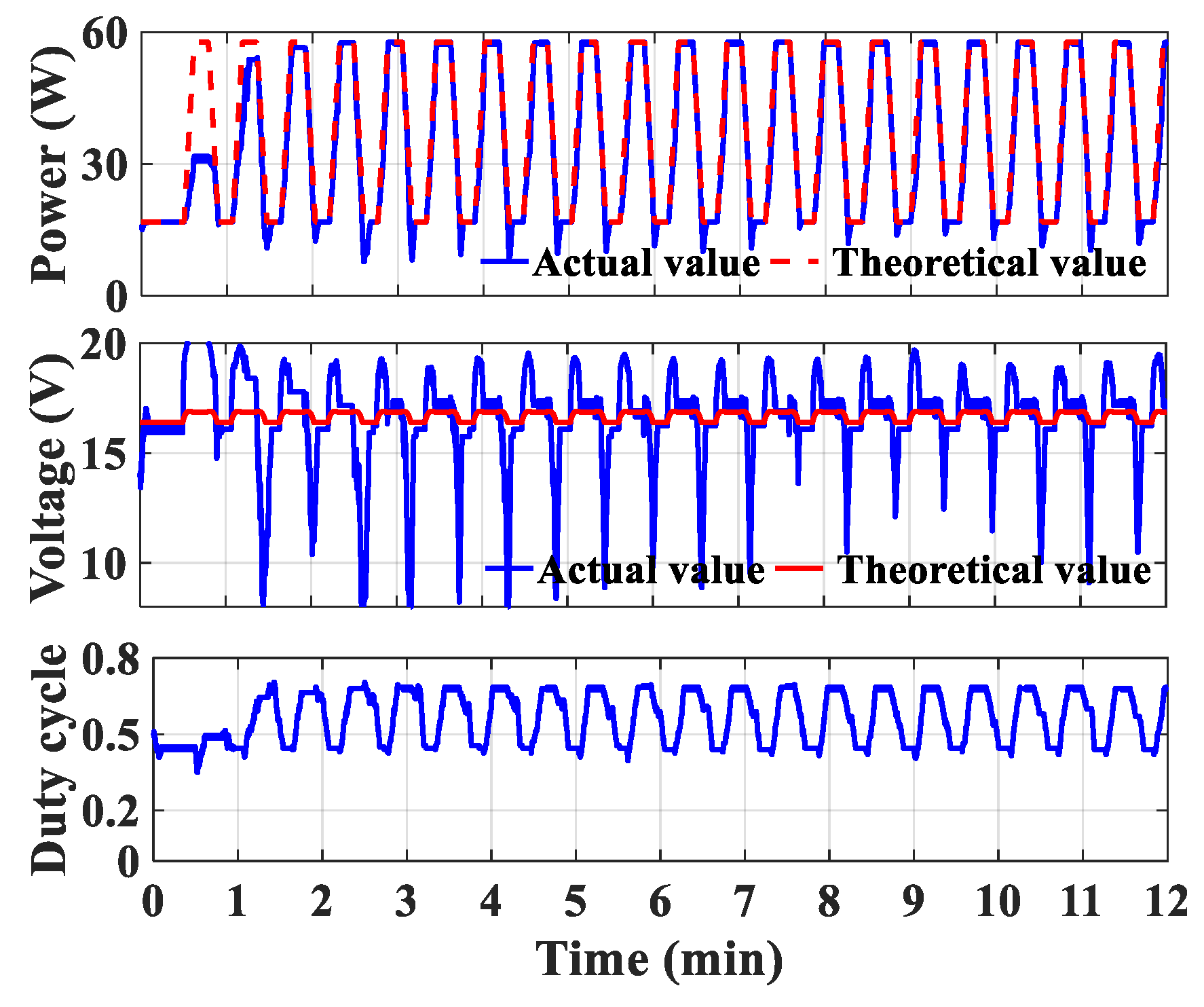
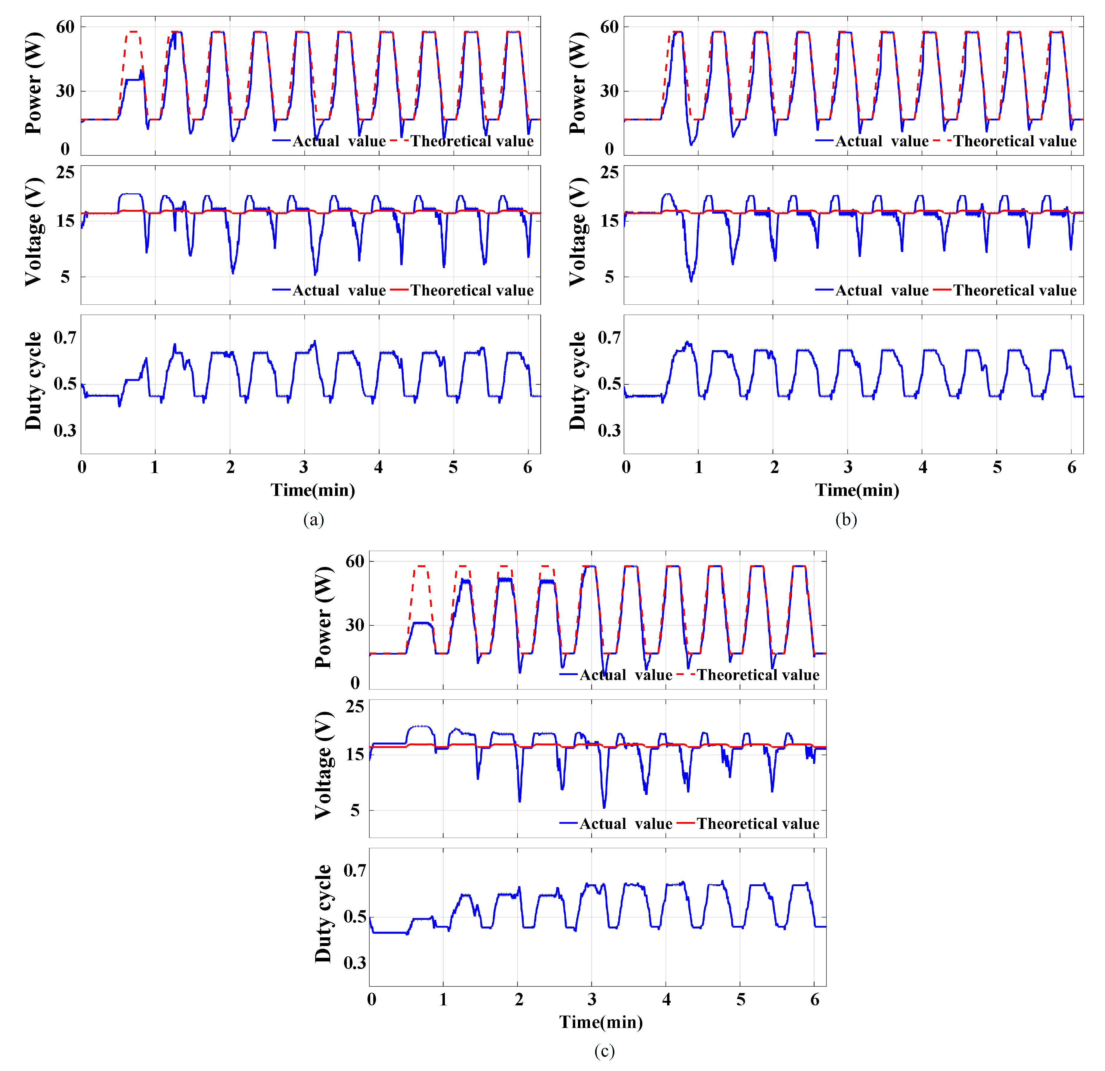
The simulation results for type 1 of the action space with different types of state spaces are described in Figure 13. It is seen that the first and third state spaces can lead to significant trace failure for the first pattern. Notably, the second state space mitigates voltage drop during irradiance descent, resulting in an increase in harvested energy. In comparison to the first and second state spaces, it is found that the overall efficiency of the third state space is lower, achieving successful tracking of power maximum point at high irradiance steady-state only for the fourth pattern. Generally speaking, type 2 exhibits slower tracking compared to type 1, particularly during the rise of irradiance. Efficiency variations under different Q-tables are illustrated in

Table 3. Comparisonof simulation efficiency results of different Q-tables.

	1 V and 0.1 A	1 V and 0.2 A	1.5 V and 0.1 A
Action Type 1	92.32%	95.55%	93.44%
Action Type 2	90.21%	91.90%	90.09%

.

3.3. Experimental Evaluation

Figure 10 shows the hardware in the loop (HIL) used in this experimental setup, and the TMS320F28335 model microcontroller produced by Texas Instruments is used.

The voltage and current from the MT6061 are converted by an analog-to-digital converter (ADC) and sampled by the microcontroller, and then a PWM control signal is generated by the controller area network (CAN). The simulation process is carried out through the Simulink Matlab 2018b.

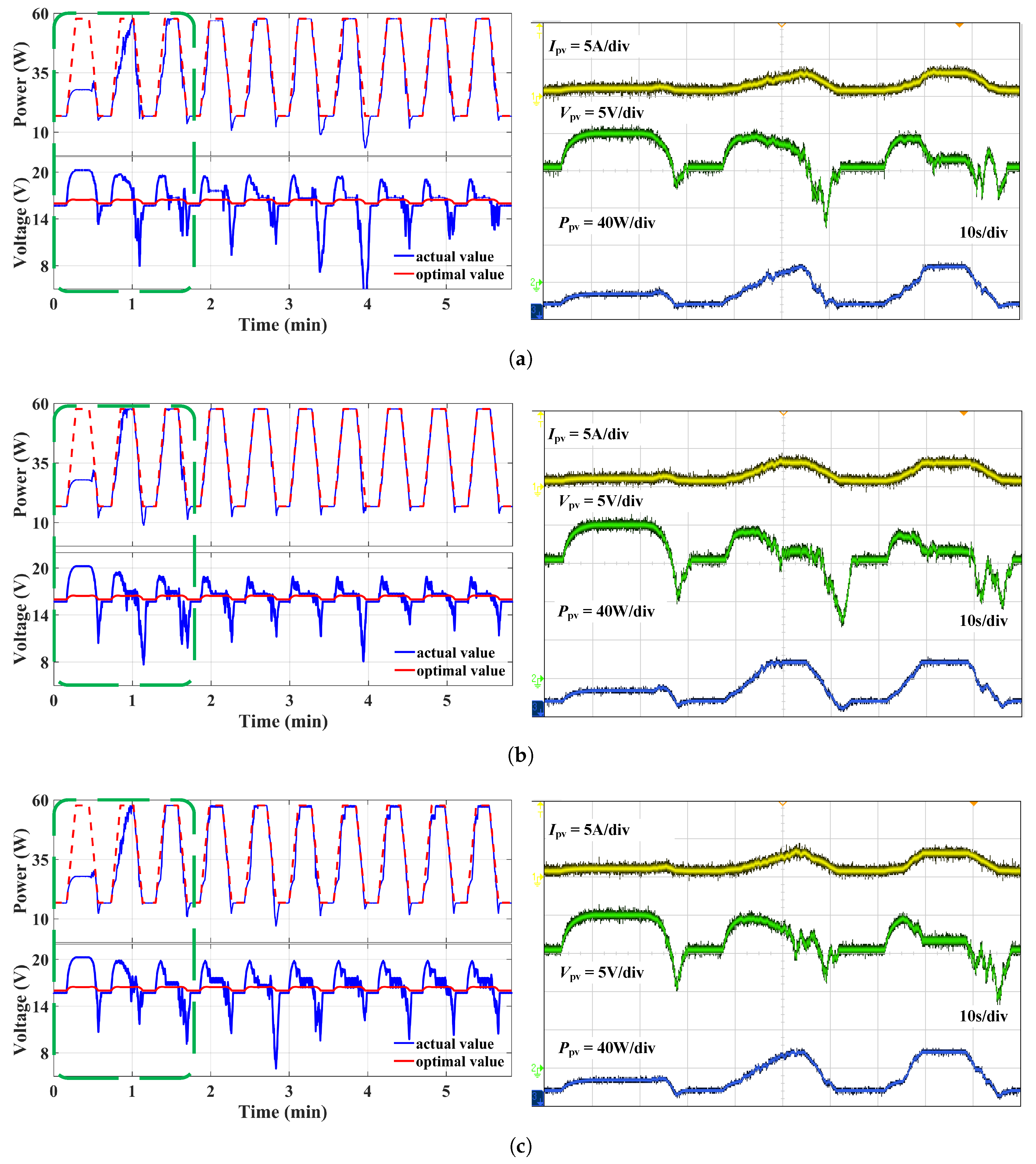
This experiment was conducted on the MT6016 machine and obtained the same experimental test parameters as the simulation results. Figure 14 and Figure 15 show the power and voltage waveforms measured according to the En50530 test procedure. Where the green dashed box indicates the initial learning iteration phase of the Q-table. It also reflects the learning speed for different discretizations.The simulation results are roughly the same as the experimental results in the type 1 action space. The second type’s efficiency is 93.78%, which is higher than 90.77% of the first type and 90.78% of the third type.

It is noteworthy that the smaller the discrete value, the closer the working point is to the MPP, thus reducing power loss. However, when the discretization value is smaller rather than larger, it requires a longer convergence time. Therefore, achieving fast convergence and high tracking accuracy can be achieved by selecting an appropriate discretization value.

Figure 14 presents the experimental results for the type 2 action space with different kinds of state space. The efficiency of the second kind, at 88.55%, is the highest among the three kinds of state space, which is similar to the type 1 action space. Regardless of how the state space is sampled, type 2 leads to a lower efficiency compared to type 1. Thus, type 1 is better than type 2. Furthermore, due to sampling smaller step sizes (a1 and a5), the tracking speed is slow during the uphill part of the second pattern. But as the experience accumulates, the tracking speed improves greatly during the uphill part of the irradiance increasing process, and its efficiency increases. In addition, unlike in type 1, the voltage dip during the downhill slope is more severe in type 2.

Table 4. Comparisonof experiment efficiency results of different Q-tables.

	1 V and 0.1 A	1 V and 0.2 A	1.5 V and 0.1 A
Action Type 1	90.77%	93.78%	90.78%
Action Type 2	87.35%	88.55%	85.98%

shows the efficiency under different Q-tables.

4. Conclusions

In this paper, six kinds of Q-tables of the RL-MPPT method under the En50530 test procedure are discussed. By comparing the simulation and experimental results with the other two kinds of discretization value, it is shown that the highest efficiency can be achieved when the discretization value states are 1 V and 0.2 A. Additionally, the type 1 action space can lead to higher efficiency than the type 2 action space. Thus, this work recommends that the Q-table be set to a moderate resolution of state space and type 1 action space, which can lead to less power loss.