


Quantitative Prediction of Rock Pore-Throat Radius Based on Deep Neural Network


Abstract
:1. Introduction
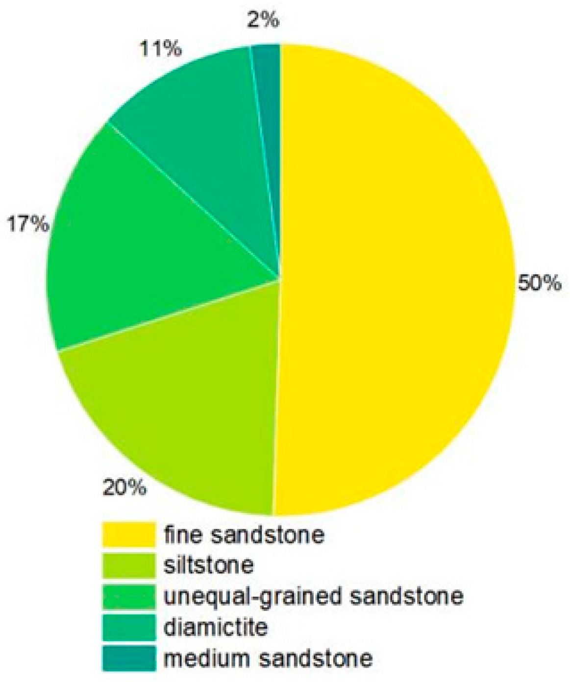
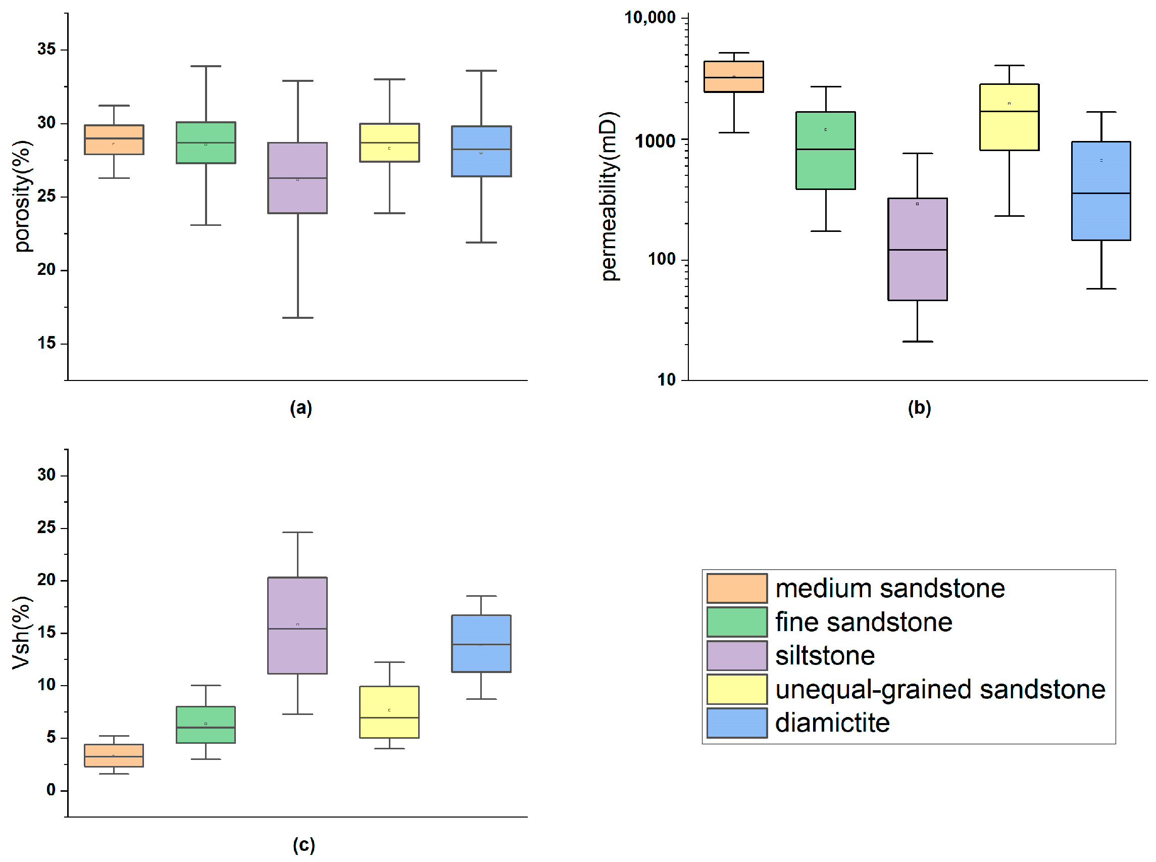
2. Materials
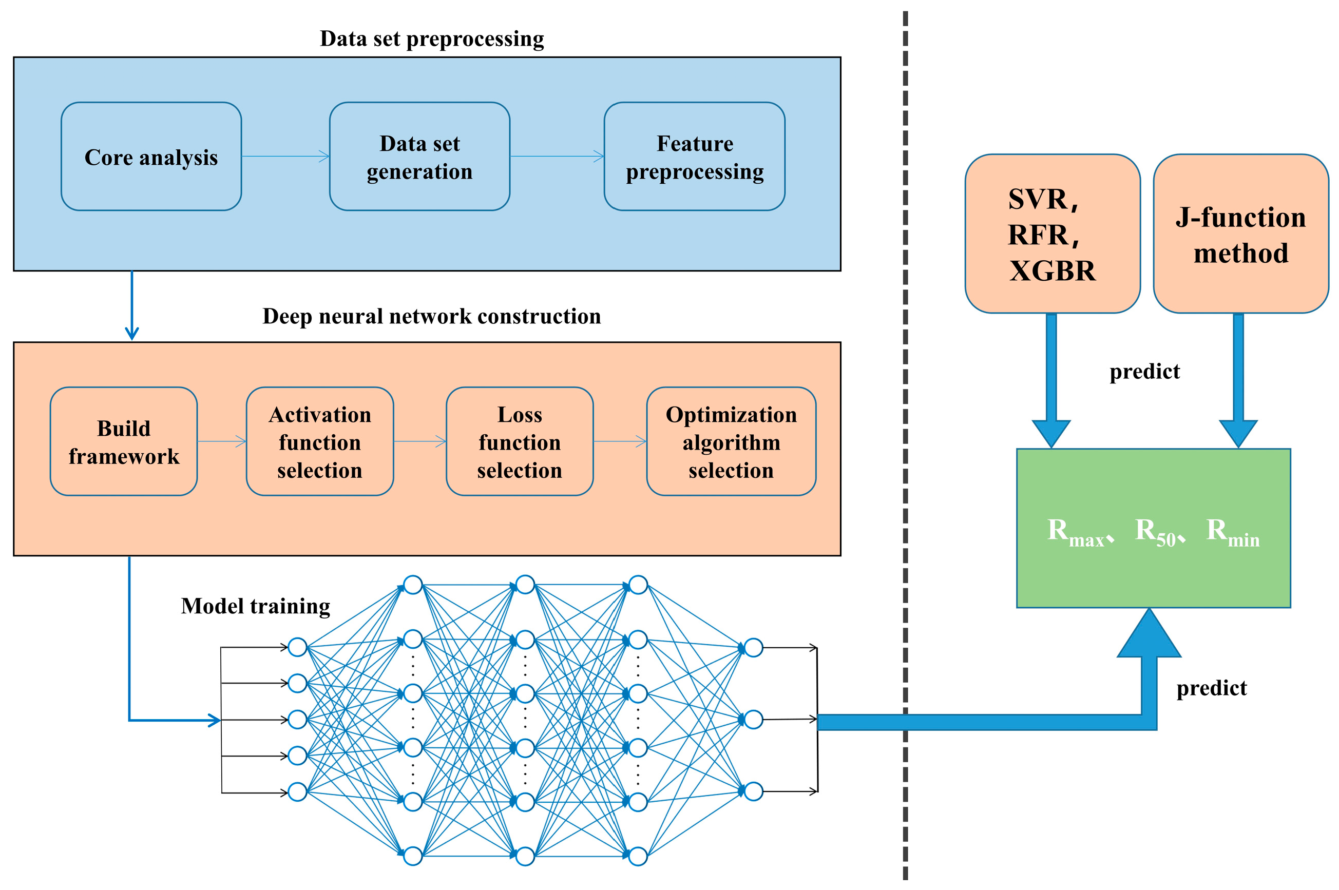
3. Method
3.1. Data Analysis and Preprocessing
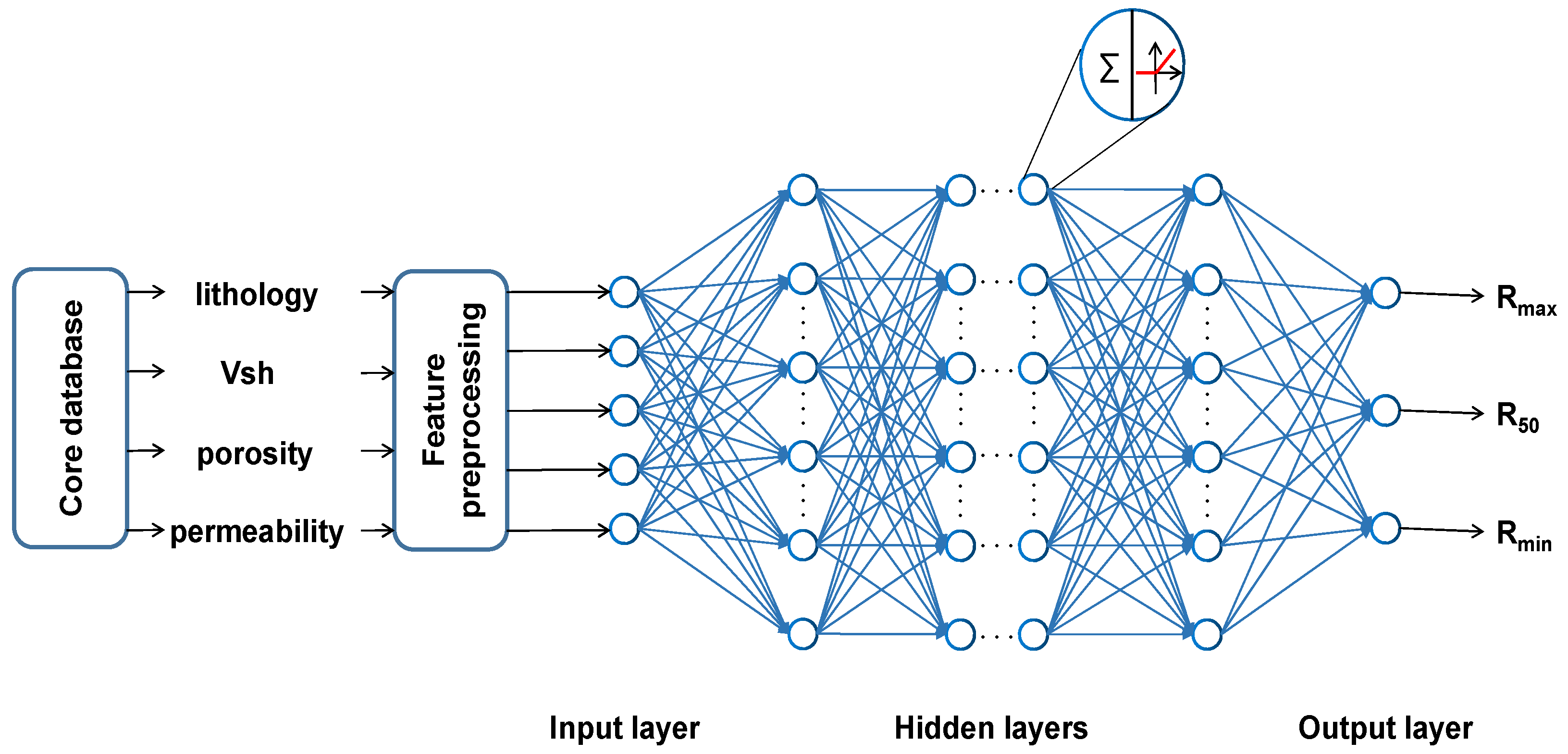
3.2. Deep Neural Network
3.3. Selection of DNN Key Elements
3.3.1. Activation Function Selection
3.3.2. Loss Function Selection
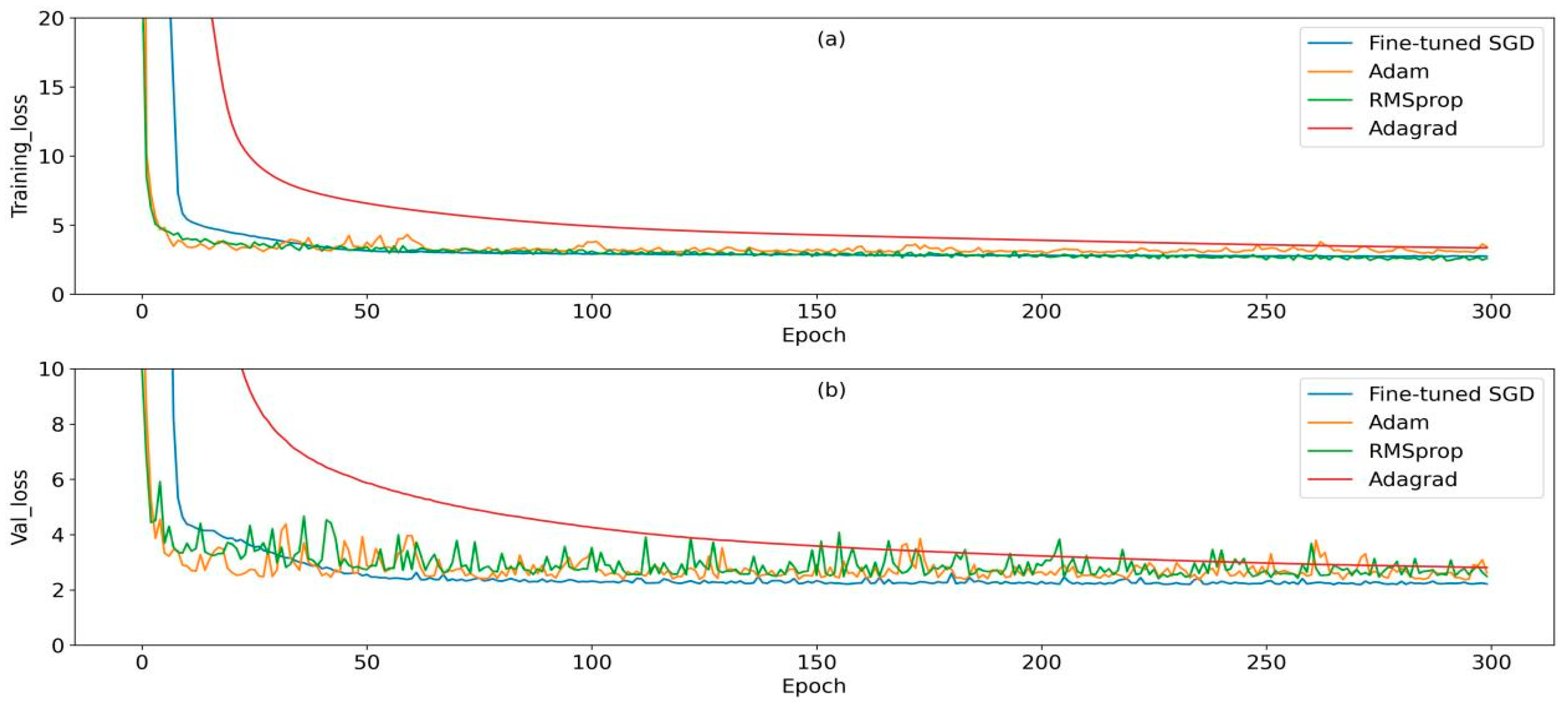
3.3.3. Optimization Algorithm Selection
3.4. Pore-Throat Radius Prediction by Deep Neural Network
3.5. Pore-Throat Radius Prediction by Comparable Machine Learning Methods
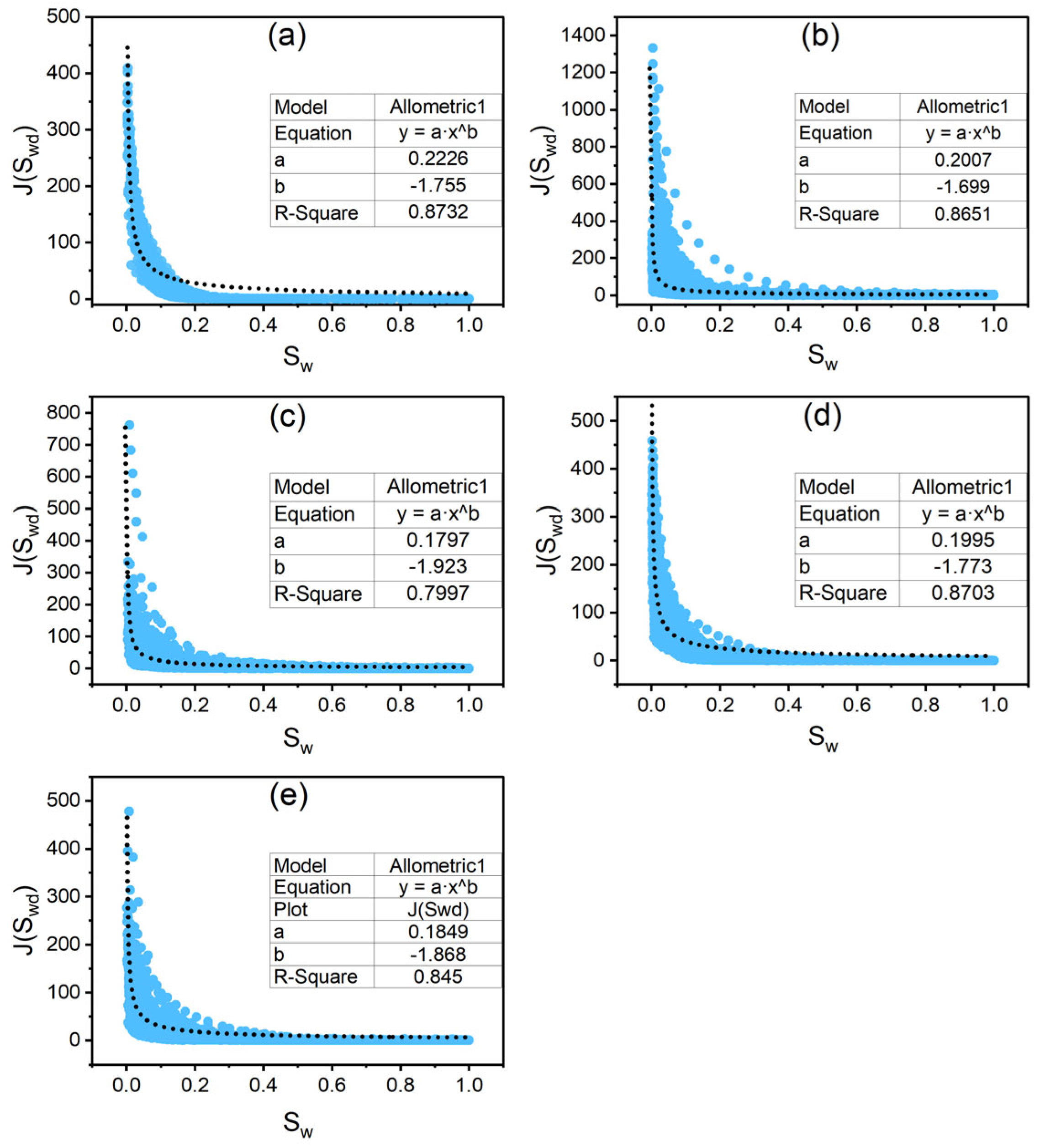
3.6. Pore-Throat Radius Prediction by J-Function Method
4. Results and Discussion
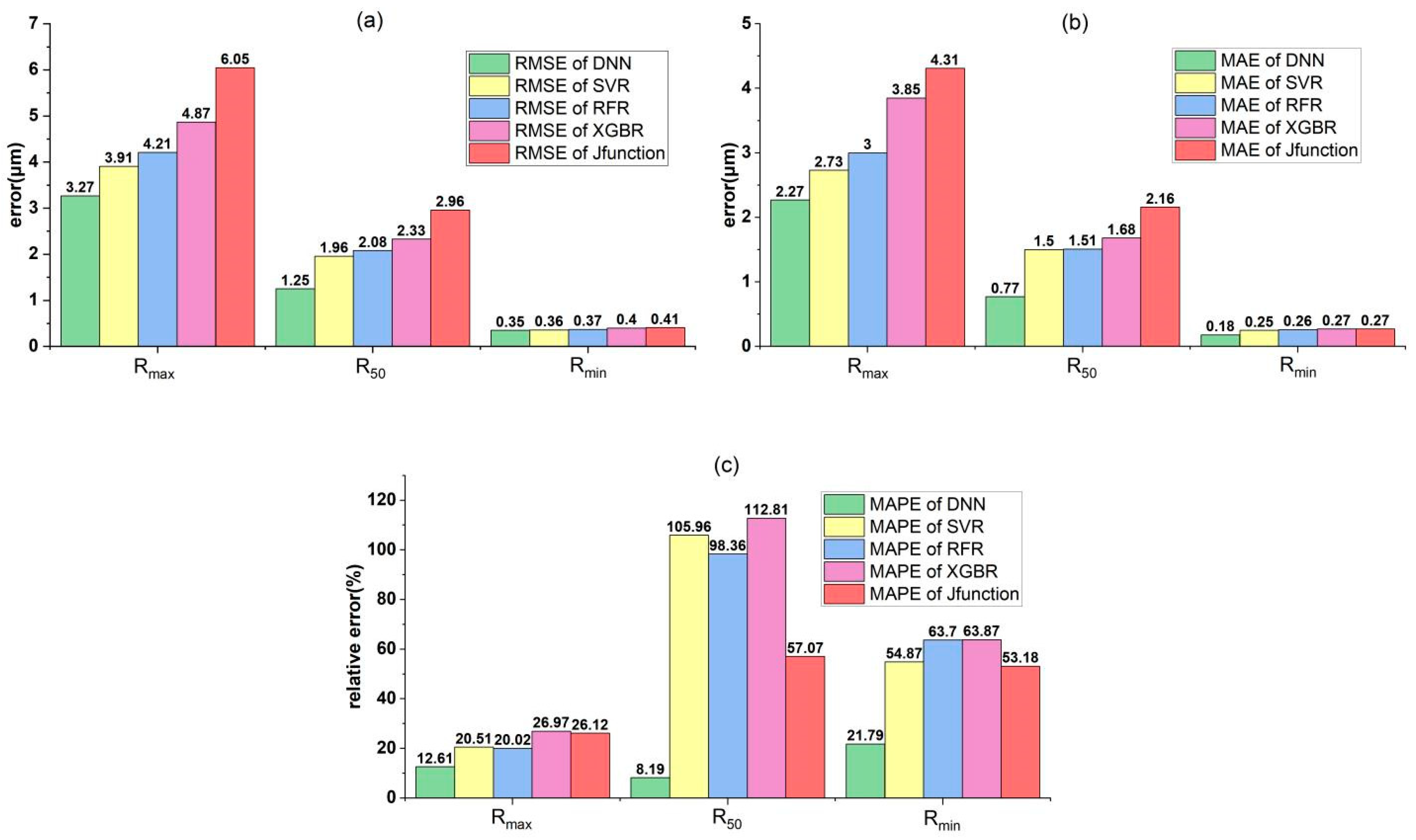
4.1. Predictive Performance Analysis
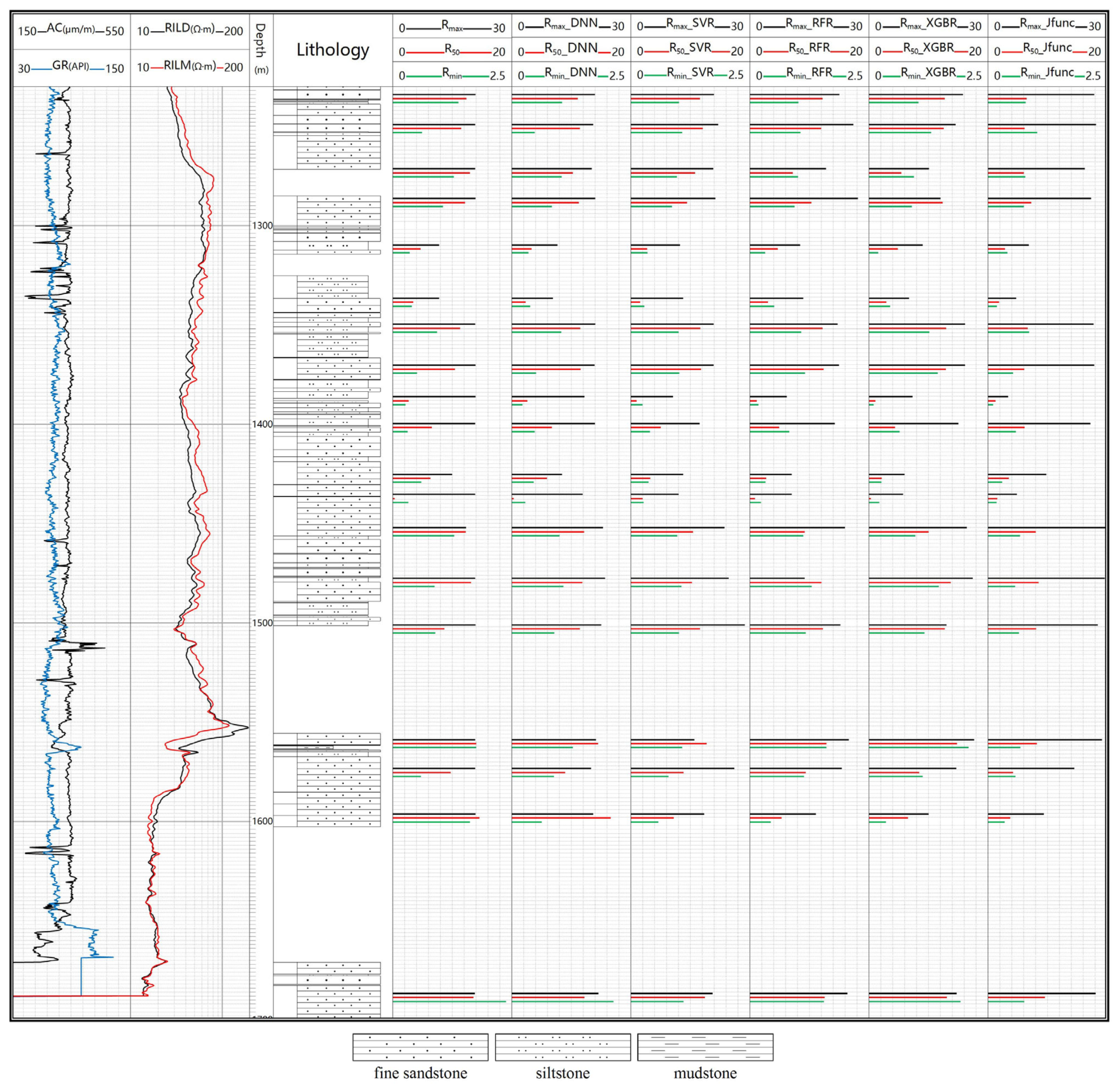
4.2. Analysis of Actual Prediction
5. Conclusions
Author Contributions
Funding
Data Availability Statement
Acknowledgments
Conflicts of Interest
References
- Morrow, N.R. Small-scale packing heterogeneities in porous sedimentary rocks. AAPG Bull. 1971, 55, 514–522. [Google Scholar]
- Pettijohn, F.J.; Potter, P.E.; Siever, R. Sand and Sandstone; Springer Science & Business Media: Berlin/Heidelberg, Germany, 2012. [Google Scholar]
- Yinan, Q. Developments in reservoir sedimentology of continental clastic rocks in China. Acta Sedimentol. Sin. 1992, 10, 16–24. [Google Scholar]
- Li, J.; Liu, Y.; Gao, Y.; Cheng, B.; Meng, F.; Xu, H. Effects of microscopic pore structure heterogeneity on the distribution and morphology of remaining oil. Pet. Explor. Dev. 2018, 45, 1112–1122. [Google Scholar] [CrossRef]
- Liu, G.; Xie, S.; Tian, W.; Wang, J.; Li, S.; Wang, Y.; Yang, D. Effect of pore-throat structure on gas-water seepage behaviour in a tight sandstone gas reservoir. Fuel 2022, 310, 121901. [Google Scholar] [CrossRef]
- Yuan, C.; Pu, W.; Varfolomeev, M.A.; Wei, J.; Zhao, S.; Cao, L.N. Deformable microgel for enhanced oil recovery in high-temperature and ultrahigh-salinity reservoirs: How to design the particle size of microgel to achieve its optimal match with pore throat of porous media. SPE J. 2021, 26, 2053–2067. [Google Scholar] [CrossRef]
- Gao, Z.; Hu, Q. Estimating permeability using median pore-throat radius obtained from mercury intrusion porosimetry. J. Geophys. Eng. 2013, 10, 025014. [Google Scholar] [CrossRef]
- Lala, A.M.S.; El-Sayed, N.A. Controls of pore throat radius distribution on permeability. J. Pet. Sci. Eng. 2017, 157, 941–950. [Google Scholar] [CrossRef]
- Gong, Y.; Liu, K.; Zhuo, Q. Pore throat radius cutoffs from depression to uplift zones: A case study of the tight oil reservoir from the Songliao Basin, NE China. J. Asian Earth. Sci. 2023, 246, 105576. [Google Scholar] [CrossRef]
- Xiao, Q.; Wang, Z.; Yang, Z.; Xiang, Z.; Liu, Z.; Yang, W. Novel method for determining the lower producing limits of pore-throat radius and permeability in tight oil reservoirs. Energy. Rep. 2021, 7, 1651–1656. [Google Scholar] [CrossRef]
- Ali, L.; Barrufet, M.A. Study of pore structure modification using environmental scanning electron microscopy. J. Pet. Sci. Eng. 1995, 12, 323–338. [Google Scholar] [CrossRef]
- Chandra, D.; Vishal, V. A critical review on pore to continuum scale imaging techniques for enhanced shale gas recovery. Earth Sci. Rev. 2021, 217, 103638. [Google Scholar] [CrossRef]
- Hu, C.; Yang, F.; Ning, Z.; Wang, B.; Peng, K.; Liu, H. Characterization of microscopic pore structures in shale reservoirs. Acta Pet. Sin. 2013, 34, 301. [Google Scholar]
- Ivanova, A.; Mitiurev, N.; Cheremisin, A.; Orekhov, A.; Kamyshinsky, R.; Vasiliev, A. Characterization of organic layer in oil carbonate reservoir rocks and its effect on microscale wetting properties. Sci. Rep. 2019, 9, 10667. [Google Scholar] [CrossRef]
- Yang, X.; Wang, J.; Zhu, C.; He, M.; Gao, Y. Effect of wetting and drying cycles on microstructure of rock based on SEM. Environ. Earth Sci. 2019, 78, 183. [Google Scholar] [CrossRef]
- Clarkson, C.; Solano, N.; Bustin, R.; Bustin, A.; Chalmers, G.; He, L.; Melnichenko, Y.; Radliński, A.; Blach, T. Pore structure characterization of North American shale gas reservoirs using USANS/SANS, gas adsorption, and mercury intrusion. Fuel 2013, 103, 606–616. [Google Scholar] [CrossRef]
- Shaobo, T.H.Z.S.L.; Hong, Z. Determination of organic-rich shale pore features by mercury injection and gas adsorption methods. Acta Pet. Sin. 2012, 33, 419. [Google Scholar]
- Timur, A. Pulsed nuclear magnetic resonance studies of porosity, movable fluid, and permeability of sandstones. J. Pet. Technol. 1969, 21, 775–786. [Google Scholar] [CrossRef]
- Golsanami, N.; Sun, J.; Zhang, Z. A review on the applications of the nuclear magnetic resonance (NMR) technology for investigating fractures. J. Appl. Geophys. 2016, 133, 30–38. [Google Scholar] [CrossRef]
- Arns, C.H.; Bauget, F.; Sakellariou, A.; Senden, T.J.; Sheppard, A.P.; Sok, R.M.; Ghous, A.; Pinczewski, W.V.; Knackstedt, M.A.; Kelly, J.C. Digital core laboratory: Petrophysical analysis from 3D imaging of reservoir core fragments. Petrophysics 2005, 46, 260–277. [Google Scholar]
- Knackstedt, M.A.; Arns, C.H.; Limaye, A.; Sakellariou, A.; Senden, T.J.; Sheppard, A.P.; Sok, R.M.; Pinczewski, W.V.; Bunn, G.F. Digital Core Laboratory: Properties of reservoir core derived from 3D images. In Proceedings of the SPE Asia Pacific Conference on Integrated Modelling for Asset Management, Kuala Lumpur, Malaysia, 29–30 March 2004. [Google Scholar]
- Arns, C.H.; Knackstedt, M.A.; Pinczewski, W.; Martys, N.S. Virtual permeametry on microtomographic images. J. Pet. Sci. Eng. 2004, 45, 41–46. [Google Scholar] [CrossRef]
- Fredrich, J.; Menéndez, B.; Wong, T.-F. Imaging the pore structure of geomaterials. Science 1995, 268, 276–279. [Google Scholar] [CrossRef] [PubMed]
- Zhao, J.; Cui, L.; Chen, H.; LI, N.; Wang, Z.; Ma, Y.; Du, G. Quantitative characterization of rock microstructure of digital core based on CT scanning. Geoscience 2020, 34, 1205. [Google Scholar]
- Okabe, H.; Blunt, M.J. Pore space reconstruction using multiple-point statistics. J. Pet. Sci. Eng. 2005, 46, 121–137. [Google Scholar] [CrossRef]
- Arand, F.; Hesser, J. Accurate and efficient maximal ball algorithm for pore network extraction. Comput. Geosci. 2017, 101, 28–37. [Google Scholar] [CrossRef]
- Al-Kharusi, A.S.; Blunt, M.J. Network extraction from sandstone and carbonate pore space images. J. Pet. Sci. Eng. 2007, 56, 219–231. [Google Scholar] [CrossRef]
- Liu, J.; Regenauer-Lieb, K. Application of percolation theory to microtomography of rocks. Earth Sci. Rev. 2021, 214, 103519. [Google Scholar] [CrossRef]
- Borello, E.S.; Peter, C.; Panini, F.; Viberti, D. Application of A* algorithm for microstructure and transport properties characterization from 3D rock images. Energy 2022, 239, 122151. [Google Scholar] [CrossRef]
- Liang, Y.; Hu, P.; Wang, S.; Song, S.; Jiang, S. Medial axis extraction algorithm specializing in porous media. Powder Technol. 2019, 343, 512–520. [Google Scholar] [CrossRef]
- Rabbani, A.; Mostaghimi, P.; Armstrong, R.T. Pore network extraction using geometrical domain decomposition. Adv. Water Resour. 2019, 123, 70–83. [Google Scholar] [CrossRef]
- Xiao, Q.; Yang, Z.; Wang, Z.; Qi, Z.; Wang, X.; Xiong, S. A full-scale characterization method and application for pore-throat radius distribution in tight oil reservoirs. J. Pet. Sci. Eng. 2020, 187, 106857. [Google Scholar] [CrossRef]
- Qu, Y.; Sun, W.; Wu, H.; Huang, S.; Li, T.; Ren, D.; Chen, B. Impacts of pore-throat spaces on movable fluid: Implications for understanding the tight oil exploitation process. Mar. Pet. Geol. 2022, 137, 105509. [Google Scholar] [CrossRef]
- Wei, Q.; Li, X.; Zhang, J.; Hu, B.; Zhu, W.; Liang, W.; Sun, K. Full-size pore structure characterization of deep-buried coals and its impact on methane adsorption capacity: A case study of the Shihezi Formation coals from the Panji Deep Area in Huainan Coalfield, Southern North China. J. Pet. Sci. Eng. 2019, 173, 975–989. [Google Scholar] [CrossRef]
- Brooks, R.H. Hydraulic Properties of Porous Media; Colorado State University: Fort Collins, CO, USA, 1965. [Google Scholar]
- Leverett, M. Capillary behavior in porous solids. Trans. AIME 1941, 142, 152–169. [Google Scholar] [CrossRef]
- Aguilera, R. Incorporating capillary pressure, pore throat aperture radii, height above free-water table, and winland r 35 values on Pickett plots. AAPG Bull. 2002, 86, 605–624. [Google Scholar]
- Kolodzie, S. Analysis of pore throat size and use of the Waxman-Smits equation to determine OOIP in Spindle Field, Colorado. In Proceedings of the SPE Annual Technical Conference and Exhibition, Dallas, TX, USA, 21–24 September 1980. [Google Scholar]
- Ziarani, A.S.; Aguilera, R. Pore-throat radius and tortuosity estimation from formation resistivity data for tight-gas sandstone reservoirs. J. Appl. Geophys. 2012, 83, 65–73. [Google Scholar] [CrossRef]
- Yu, S.; Ma, J. Deep learning for geophysics: Current and future trends. Rev. Geophys. 2021, 59, e2021RG000742. [Google Scholar] [CrossRef]
- Saikia, P.; Baruah, R.D.; Singh, S.K.; Chaudhuri, P.K. Artificial Neural Networks in the domain of reservoir characterization: A review from shallow to deep models. Comput. Geosci. 2020, 135, 104357. [Google Scholar] [CrossRef]
- Li, Y.; Lian, P.Q.; Xue, Z.J.; Dai, C. Application status and prospect of big data and artificial intelligence in oil and gas field development. J. China Univ. Pet. Ed. Nat. Sci. 2020, 44, 1–11. [Google Scholar]
- Wolpert, D.H. The lack of a priori distinctions between learning algorithms. Neural Comput. 1996, 8, 1341–1390. [Google Scholar] [CrossRef]
- Naeini, E.Z.; Green, S.; Russell-Hughes, I.; Rauch-Davies, M. An integrated deep learning solution for petrophysics, pore pressure, and geomechanics property prediction. Lead. Edge 2019, 38, 53–59. [Google Scholar] [CrossRef]
- Li, T.; Wang, Z.; Wang, R.; Yu, N. Pore type identification in carbonate rocks using convolutional neural network based on acoustic logging data. Neural Comput. Appl. 2021, 33, 4151–4163. [Google Scholar] [CrossRef]
- Miller, R.S.; Rhodes, S.; Khosla, D.; Nino, F. Application of artificial intelligence for depositional facies recognition-Permian basin. In Proceedings of the SPE/AAPG/SEG Unconventional Resources Technology Conference, Denver, CO, USA, 22–24 July 2019. [Google Scholar]
- Pham, N.; Wu, X.; Zabihi Naeini, E. Missing well log prediction using convolutional long short-term memory network. Geophysics 2020, 85, WA159–WA171. [Google Scholar] [CrossRef]
- Zhang, D.; Yuntian, C.; Jin, M. Synthetic well logs generation via Recurrent Neural Networks. Pet. Explor. Dev. 2018, 45, 629–639. [Google Scholar] [CrossRef]
- Gao, X.; He, W.; Hu, Y. Modeling of meandering river deltas based on the conditional generative adversarial network. J. Pet. Sci. Eng. 2020, 193, 107352. [Google Scholar] [CrossRef]
- Zhang, T.-F.; Tilke, P.; Dupont, E.; Zhu, L.-C.; Liang, L.; Bailey, W. Generating geologically realistic 3D reservoir facies models using deep learning of sedimentary architecture with generative adversarial networks. Pet. Sci. 2019, 16, 541–549. [Google Scholar] [CrossRef]
- Lu, H.; Hu, S.; Zhang, L.; Tang, H.; Yang, T.; Zhao, Y.; Li, L.; Zhao, F. Prediction of the pore structure by machine learning techniques in the carbonate reservoirs in Iraq H oilfield. Geol. J. 2023, 58, 2427–2437. [Google Scholar] [CrossRef]
- Wang, Y.; Sun, S. Multiscale pore structure characterization based on SEM images. Fuel 2021, 289, 119915. [Google Scholar] [CrossRef]
- Pan, S.; Zheng, Z.; Guo, Z.; Luo, H. An optimized XGBoost method for predicting reservoir porosity using petrophysical logs. J. Pet. Sci. Eng. 2022, 208, 109520. [Google Scholar] [CrossRef]
- Alqahtani, N.; Alzubaidi, F.; Armstrong, R.T.; Swietojanski, P.; Mostaghimi, P. Machine learning for predicting properties of porous media from 2d X-ray images. J. Pet. Sci. Eng. 2020, 184, 106514. [Google Scholar] [CrossRef]
- Alqahtani, N.; Armstrong, R.T.; Mostaghimi, P. Deep learning convolutional neural networks to predict porous media properties. In Proceedings of the SPE Asia Pacific Oil and Gas Conference and Exhibition, Brisbane, Australia, 23–25 October 2018. [Google Scholar]
- Misbahuddin, M. Estimating petrophysical properties of shale rock using conventional neural networks CNN. In Proceedings of the SPE Annual Technical Conference and Exhibition, Virtual, 26–29 October 2020. [Google Scholar]
- Iraji, S.; Soltanmohammadi, R.; Matheus, G.F.; Basso, M.; Vidal, A.C. Application of unsupervised learning and deep learning for rock type prediction and petrophysical characterization using multi-scale data. Geoenergy Sci. Eng. 2023, 230, 212241. [Google Scholar] [CrossRef]
- Zhou, Y.; Yin, D.; Cao, R.; Zhang, C. The mechanism for pore-throat scale emulsion displacing residual oil after water flooding. J. Pet. Sci. Eng. 2018, 163, 519–525. [Google Scholar] [CrossRef]
- Washburn, E.W. Note on a method of determining the distribution of pore sizes in a porous material. Proc. Natl. Acad. Sci. USA 1921, 7, 115–116. [Google Scholar] [CrossRef] [PubMed]
- Purcell, W. Capillary pressures-their measurement using mercury and the calculation of permeability therefrom. J. Pet. Technol. 1949, 1, 39–48. [Google Scholar] [CrossRef]
- Wells, J.; Amaefule, J. Capillary pressure and permeability relationships in tight gas sands. In Proceedings of the SPE/DOE Low Permeability Gas Reservoirs Symposium, Denver, CO, USA, 19–22 May 1985. [Google Scholar]
- Samek, W.; Montavon, G.; Lapuschkin, S.; Anders, C.J.; Müller, K.R. Explaining deep neural networks and beyond: A review of methods and applications. Proc. IEEE 2021, 109, 247–278. [Google Scholar] [CrossRef]
- Nassif, A.B.; Shahin, I.; Attili, I.; Azzeh, M.; Shaalan, K. Speech recognition using deep neural networks: A systematic review. IEEE Access 2019, 7, 19143–19165. [Google Scholar] [CrossRef]
- Srinidhi, C.L.; Ciga, O.; Martel, A.L. Deep neural network models for computational histopathology: A survey. Med. Image Anal. 2021, 67, 101813. [Google Scholar] [CrossRef]
- Montavon, G.; Samek, W.; Müller, K.-R. Methods for interpreting and understanding deep neural networks. Digit. Signal Process. 2018, 73, 1–15. [Google Scholar] [CrossRef]
- Sze, V.; Chen, Y.-H.; Yang, T.-J.; Emer, J.S. Efficient processing of deep neural networks: A tutorial and survey. Proc. IEEE 2017, 105, 2295–2329. [Google Scholar] [CrossRef]
- Jiang, X.; Pang, Y.; Li, X.; Pan, J.; Xie, Y. Deep neural networks with elastic rectified linear units for object recognition. Neurocomputing 2018, 275, 1132–1139. [Google Scholar] [CrossRef]
- Weng, L.; Zhang, H.; Chen, H.; Song, Z.; Hsieh, C.J.; Daniel, L.; Boning, D.; Dhillon, I. Towards fast computation of certified robustness for relu networks. In Proceedings of the 35th International Conference on Machine Learning, PMLR 80, Stockholm, Sweden, 10–15 July 2018. [Google Scholar]
- Esmaeili, A.; Marvasti, F. A novel approach to quantized matrix completion using huber loss measure. IEEE Signal Process. Lett. 2019, 26, 337–341. [Google Scholar] [CrossRef]
- Gupta, D.; Hazarika, B.B.; Berlin, M. Robust regularized extreme learning machine with asymmetric Huber loss function. Neural Comput. Appl. 2020, 32, 12971–12998. [Google Scholar] [CrossRef]
- Smola, A.J.; Schölkopf, B. A tutorial on support vector regression. Stat. Comput. 2004, 14, 199–222. [Google Scholar] [CrossRef]

| Method | Input Variable | Prediction | Source | |
|---|---|---|---|---|
| Petrophysics-based Methods | empirical fitting formulae | porosity, permeability | R35 | [37,38,39] |
| Indirect prediction by bound water film thickness | bound water volume, inner surface area | lower limits of pore-throat radius | [10] | |
| Machine learning Methods | 5 layers CNN | micro-CT images | average pore size | [54,55] |
| 4 layers CNN | grayscale SEM images | average pore size | [56] | |
| componential optimized deep neural network | lithology, porosity, permeability, and shale volume | Rmax, R50 and Rmin | This paper |
| Lithology | Medium Sandstone | Fine Sandstone | Siltstone | Unequal-Grained Sandstone | Diamictite |
|---|---|---|---|---|---|
| Median grain size (μm) | 235–344 | 86–245 | 11–98 | 101–261 | 29–162 |
| Loss Function | Value |
|---|---|
| Huber | 2.41 |
| MSE (L2) | 3.83 |
| MAE (L1) | 2.97 |
| Data Preprocessing | Activation Function | Evaluation Metrics | Optimization Algorithm | Loss Function | Cross Validation | Regularization Method | ||
|---|---|---|---|---|---|---|---|---|
| Discrete Variable | Continuous Variable | |||||||
| one-hot encoding | Z-score standardization | ReLU | RMSE, MAE, MAPE | Fine-tuned SGD | Huber loss | 10-fold Stratified K-Fold | ReduceLROnPlateau | EarlyStopping |
| Structural Hyperparameter | Value | ||
|---|---|---|---|
| Rmax | R50 | Rmin | |
| Hidden layers | 7 | ||
| Nodes of each layer | 16, 64, 128, 128, 64, 64, 32 | ||
| Initial learning rate | 0.001 | ||
| Epochs | 100 | 200 | 140 |
| Batch size | 300 | 50 | 200 |
| Method | Running Time for Training (s) | Running Time for Predicting (s) |
|---|---|---|
| DNN | 51.34 | 3.44 |
| SVR | 34.81 | 2.56 |
| RFR | 29.73 | 3.15 |
| XGBR | 33.58 | 2.92 |
| J-function | / | >3600 |
| Mean Absolute Errors | Methods | ||||
|---|---|---|---|---|---|
| DNN | SVR | RFR | XGB | J-Function | |
| Rmax | 1.195 | 3.034 | 4.012 | 4.176 | 6.410 |
| R50 | 0.951 | 2.007 | 2.028 | 2.072 | 4.093 |
| Rmin | 0.207 | 0.329 | 0.351 | 0.406 | 0.434 |
Disclaimer/Publisher’s Note: The statements, opinions and data contained in all publications are solely those of the individual author(s) and contributor(s) and not of MDPI and/or the editor(s). MDPI and/or the editor(s) disclaim responsibility for any injury to people or property resulting from any ideas, methods, instructions or products referred to in the content. |
© 2023 by the authors. Licensee MDPI, Basel, Switzerland. This article is an open access article distributed under the terms and conditions of the Creative Commons Attribution (CC BY) license (https://creativecommons.org/licenses/by/4.0/).
Share and Cite
Hong, Y.; Li, S.; Wang, H.; Liu, P.; Cao, Y. Quantitative Prediction of Rock Pore-Throat Radius Based on Deep Neural Network. Energies 2023, 16, 7277. https://doi.org/10.3390/en16217277
Hong Y, Li S, Wang H, Liu P, Cao Y. Quantitative Prediction of Rock Pore-Throat Radius Based on Deep Neural Network. Energies. 2023; 16(21):7277. https://doi.org/10.3390/en16217277
Chicago/Turabian StyleHong, Yao, Shunming Li, Hongliang Wang, Pengcheng Liu, and Yuan Cao. 2023. "Quantitative Prediction of Rock Pore-Throat Radius Based on Deep Neural Network" Energies 16, no. 21: 7277. https://doi.org/10.3390/en16217277
APA StyleHong, Y., Li, S., Wang, H., Liu, P., & Cao, Y. (2023). Quantitative Prediction of Rock Pore-Throat Radius Based on Deep Neural Network. Energies, 16(21), 7277. https://doi.org/10.3390/en16217277