Development of an Optimal Port Crane Trajectory for Reduced Energy Consumption ^†

Abstract

This paper is concerned with the development of an optimal load-handling trajectory for port cranes. The objective is to minimize load cycle time and reduce energy consumption. Energetic macroscopic representation formalism is used to model a port crane load-handling mechanism. The crane model developed includes the mathematical model, the crane’s local control system, and a MATLAB/Simulink model for simulation. The particle swarm optimization algorithm is used to find the set of pareto optimal crane trajectories given the variation in crane size, ship size, and wind speed. Experimental validation of the crane model is conducted by comparing it with a real-world crane. Simulation results show that the optimal crane load trajectory is 38% faster and more productive than the nonoptimal crane load trajectory. Furthermore, the results show that the optimal trajectory reduces the cranes’ peak power and energy consumption by 36% when compared with the nonoptimal trajectory.

1. Introduction

This study focuses on transportation systems and specifically on energy management for port cranes. More than 70% of global trade is seaborne, and at least 50% is carried in shipping containers [1]; the containers are loaded and unloaded at the port into ships using port cranes. Figure 1 shows the context of this study through an overview of a container port terminal consisting of ships, port cranes, trucks, and smaller yard cranes.

Port cranes, also called ship-to-shore cranes, are the largest energy consumers within the port; they consume up to 40% of the port’s energy consumption [2]. Port cranes regenerate more than 50% of the energy used to lift the container when lowering it [3], and reusing the regenerative braking energy leads to improved energy efficiency. The European Council endorsed a 30% energy efficiency target and a 27% renewable energy penetration target for European ports by 2030 [2]. It is shown in [2] that peak energy consumption accounts for 25–30% of the port’s monthly electricity bill; port cranes are the biggest contributors to peak energy consumption and are therefore suitable for peak-shaving to improve energy efficiency. Port cranes are therefore selected as the subject of this study because of the significance of the port industry to global trade and the key role played by port cranes in the functioning of the port. Furthermore, due to being the biggest energy consumers, port cranes provide the best opportunity for energy savings within the port.

There has been a growing trend in the electrification of traction systems in port terminals to decrease energy consumption and increase energy efficiency and for system decarbonization [4]. Key to the electrification of traction systems is the application of energy storage systems such as batteries, supercapacitors (SCs), fuel cells, and flywheels [3,4,5]. When used alone, energy storage systems such as batteries and supercapacitors have limited power or energy density but are complementary when combined into a hybrid energy storage system (H-ESS) [5]. In addition to the energy storage systems listed above, traction applications such as port cranes regenerate energy when braking to slow the load down. The storage and reuse of regenerative braking energy can be used to improve the crane’s energy efficiency [4].

The use of more than one energy storage system (ESS) in an H-ESS requires an energy management strategy (EMS) to control the power split between the ESSs. EMSs are categorized into optimization-based or rule-based types of strategies [6]. Rule-based EMSs produce nonoptimal results, whereas global optimal EMSs produce optimal results but are computationally costly and complex [7]. Research on EMS for port crane applications is in the early stages [8]. However, port cranes have the same type of electric powertrain as other well-researched traction applications such as electric vehicles (EVs), electric buses, lifts, and electric trains [9].

A lack of usage of optimization-based EMS for port cranes is shown in [8], and studies in [10,11] have shown that rule-based EMS based on proportional–integral (PI) and set-point controllers have been widely implemented for port cranes.

In [12], a particle swarm optimization (PSO) algorithm is used to size a supercapacitor energy storage system (ESS) with the aim of crane peak power demand reduction through storage and reuse of regenerative braking energy. In [13], it is proposed that port cranes can become “near-zero energy load systems” by using the regenerative energy (RE) stored in supercapacitors as the primary energy supply and only consuming from the grid the minimum energy needed for system losses and RE shortfall. This is, however, not currently possible given the SCs’ low energy density.

It has been shown in [14] that ports can become “near-zero energy load systems” by using hydrogen energy storage systems, resulting in up to 51.8% reduction in their levelized cost of energy.

A port-level flywheel energy storage system is simulated in [15] for a group of quay cranes to reduce the groups’ maximum power demand (peak shaving). The energy storage systems used in the studies above only include the high-power-density supercapacitor or flywheel, which only achieves peak power shaving. However, the ESS does not include a high-energy-density device such as a battery to achieve energy savings and efficiency through the reuse of regenerative braking energy.

The authors developed in [16] a novel mode-based, rule-based EMS to control the power split in a port crane with three ESSs [16]. In this paper, the authors advanced this previous work in [16] by developing an optimal port crane load-handling trajectory to optimize the crane’s energy consumption.

The main research in the development of optimal trajectories for port cranes is summarized by five overhead crane load-handling trajectories in [17]. The five trajectories only consider the horizontal trolley motion of the port crane and do not consider the effects of hoisting the load. The trajectories show that overhead cranes generally have an initial acceleration period, which is followed by a period of constant velocity and, lastly, by a deceleration period when they have arrived at their load destination. The crane motions described here result in a trapezoidal-shaped nonoptimal trajectory. This study develops an optimal crane load-handling trajectory with consideration of both the horizontal and vertical crane load motions. Further research in trajectory development for other types of cranes other than port cranes has been shown in [18,19].

The development of the optimal load-handling trajectory for port cranes intuitively leads to automation of the port crane. Automation is required to remove human error in the port crane load-handling motions. The advancement in port crane automation horizontal and vertical motions is shown in [20]. The review in [20] shows that port crane productivity is directly correlated to the time it takes to move the shipping container between ship and shore. Therefore, the optimal trajectory for port cranes to be developed in this paper shall consider crane automation to minimize the cranes’ load-handling time. The study in [21] evaluates fast trajectories for handling port crane loads; however, this study uses the nonoptimal trajectory shown in Figure 1.

The most advanced studies on powertrain optimization for traction applications are for electric vehicles (EVs). These studies solve the energy management problem using various rule-based and optimization-based methods including a dynamic programming (DP) algorithm, filtration-based controller (FBC), model predictive controller (MPC), rule-based controller (RBC), fuzzy logic controller (FLC), Pontryagin’s minimum principle (PMP), and the particle swarm optimization (PSO) algorithm [22,23,24]. The advanced research for EV applications shows the gaps that exist in EMS and ESS hybridization for port crane applications.

The studies above have developed solutions to the power-train energy management problem using computational methods in terms of optimization or rule-based algorithms. To the best of the authors’ knowledge, there are no studies for port cranes in which the energy management problem is solved by finding the optimal load-handling trajectory that minimizes load-handling time and reduces crane energy consumption.

Furthermore, to study the port crane, a system modeling technique is required. Port cranes may be classified under multi-converter multi-machine systems as described in [25]. It has been shown in [25,26] that the graphical energetic macroscopic representation (EMR) formalism may be used to model multi-converter multi-machine systems. The EMR formalism is used to develop system models, local control, and EMS for complex multi-physical energetic systems [26]. EMR is a divide-and-conquer approach to system modeling that represents subsystem interaction using power flows while respecting the three principles of integral causality, interaction, and inversion [7].

Integral causality means that the output to the energetic system is a functional integral of the input; interaction principle means that subsystems interact using action and reaction variables, and the product of the variables is instantaneous power exchange between subsystems, and lastly, the inversion principle applies direct and indirect mathematic inversion of each subsystem to develop the system’s local control scheme [26]. To the best of the authors’ knowledge, there are no studies on the development of EMR-based port crane models.

This paper is structured as follows. Section 1 is the introduction. Section 2 describes the studied port crane system modeling. Section 3 develops an optimal port crane load trajectory. Section 4 presents the experimental validation. Section 5 compares the optimal and nonoptimal port crane trajectories. Section 6 shows the simulation results, and Section 7 presents the conclusion.

2. Port Crane System Modeling

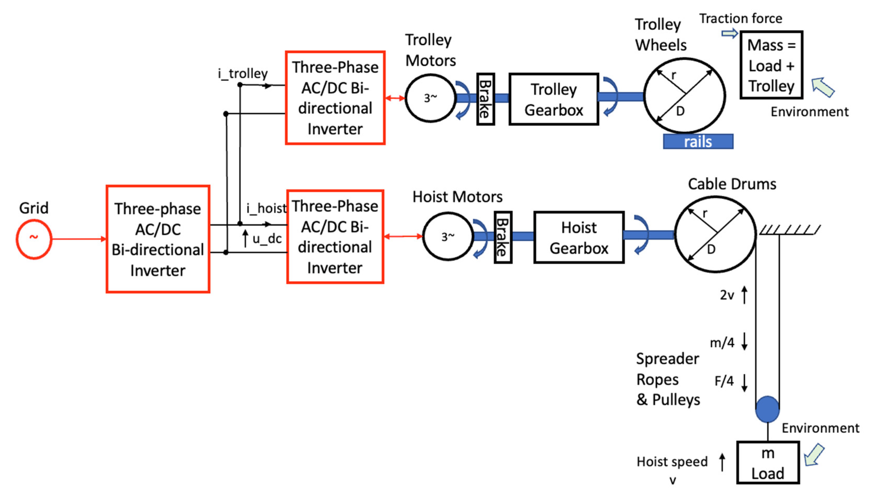
2.1. Port Crane Electromechanical System Description

Figure 2 shows the system under study. It consists of the load-handling system of a ship-to-shore (STS) crane, which is the biggest port crane. Most port cranes crane currently have a grid supply as the only energy source. A three-phase AC/DC bidirectional inverter is used to connect the DC bus to the crane motors used for propulsion to hoist and move the crane load through the hoisting and trolley systems consisting of the gearbox, drums, ropes, pulleys, and spreader systems. The load-handling system is assumed to represent all the mechanical dynamics of the crane. The load-handling environment consists of the braking, gravitational, and wind forces acting on the container load. The crane model has been reduced to focus on energy management study. To move the crane load between ship and shore, the crane hoisting system applies a vertical or lifting force to the crane load while the trolley system applies a horizontal force.

Table 1. Port crane main parameters.

Hoist System Parameters
Load mass	65 t with shipping container
	18 t empty spreader
Hoisting Speed	1.5 m/s full-load speed
	3 m/s no-load speed
Electric drive	2 × 500 kW induction machines
	Efficiency 90%
Gearbox	Ratio 21.389
	Efficiency 85%
Cable drum diameter	1.365 m
Trolley System Parameters
Trolley Speed	3.83 m/s-maximum
Electric drive	4 × 55 kW induction machines
	Efficiency 90%
Gearbox	Ratio 21.389
	Efficiency 85%
Trolley wheels diameter	710 mm
Coefficient of friction rail-to-wheel	0.02

shows the parameters of a real-world port crane that is installed at the Cape Town Container Terminal in South Africa and has been used for MATLAB-Simulink simulations in this study. The port crane can handle loads of up to 65 t; the load is hoisted to a height of 57 m on the landside and 73 m on the shipping vessel. The crane’s energy is supplied by a 1.6 MVA on-board three-phase transformer, which steps down the incoming 11 kV grid supply to 650 V. Crane hoist speed is 90 m/min with load and 180 m/min without load. Hoist acceleration duration is about 2.5 s, and steady-state duration is about 15 s. In summary, an average port crane has a power demand of between 1 MW and 2 MW, its energy consumption is between 8 kWh and 16 kWh per 30 s load cycle, and it has a regenerative capacity of between 5 kWh and 10 kWh per load cycle. The real-world port crane used in this study burns most of the energy regenerated by the hoist motors in a braking resistor located on the DC bus. The crane also has capability to feed regenerative energy back to the grid or to the crane axillary loads such as the cabin air conditioner. Based on the 24 h operation and an average 30 containers per h [20], a typical port crane has energy consumption of 17 MWh per day or 6 GWh per year.

2.2. Port Crane Energetic Macroscopic Representation

The EMR-based port crane system model, local control, and EMS is shown in Figure 3. The EMR-based port crane model leads to a system mathematical model where the crane’s EMS and local control layers are decoupled. The EMS is at the supervisory level or higher layer than the local control system and the layers must be treated differently because of differences in their dynamics. Dynamic models for the load and DC bus capacitor are used. All other port crane components are represented by their static models. It is acceptable to reduce fast dynamical subsystems to equivalent static models by considering them to be perfectly controlled with immediate response to reference inputs, as shown in [27,28].

2.3. Port Crane Mathematical Modelling

Table 2. Port crane mathematical modeling equations.

	Hoist System Modeling
Electrical Drive	$M_{@motor\_shaft}=M_{Load}/4$	(1)
	$T_m=T_{m\_ref}$	(2)
	$i_{trac}=\frac{(T_m{\omega }_m)}{2\left(U_{dc}{\eta }_{ed}^{\gamma }\right)}\left\{ \begin{array}{c}\gamma =1 T_m{\omega }_m \ge 0 \\ \gamma =-1 T_m{\omega }_m<0 \end{array}\right.$	(3)
Gearbox	$T_{GB}=\frac{(T_m{i}_{gb})}{{\eta }_{gb}^{\gamma }}\left\{ \begin{array}{c}\gamma =1 T_m{\omega }_m \ge 0 \\ \gamma =-1 T_m{\omega }_m<0 \end{array}\right.$	(4)
	${\omega }_m=I_{gb}\times {\omega }_{drum}$	(5)
Cable drum	${\omega }_{drum}=4V_L/Di{a}_{drum}$	(6)
	$F_{hoist}=T_{GB}/R_{drum}$	(7)
Spreader System	$V_{Load}=V_{hoist}/2$	(8)
	$F_{Load}=4F_{hoist}$	(9)
Load	$F_L=M_L\frac{d}{dt}{V}_L+F_{res}$	(10)
	$M_L=M_L/4$	(11)
Environment	$F_{env}=M_{L}g+0.5\rho c_{x}A{(V_L+V_w)}^2$	(12)
	Trolley System Modeling
Electrical Drive	$i_{trolley}=\frac{(T_{m\_t}{\omega }_{m\_t})}{2\left(U_{dc}{\eta }_{ed\_t}^{\gamma }\right)}\left\{ \begin{array}{c}\gamma =1 T_{m\_t}{\omega }_{m\_t} \ge 0 \\ \gamma =-1 T_{m\_t}{\omega }_{m\_t}<0 \end{array}\right.$	(13)
Gearbox	$T_{GB\_t}=\frac{(T_{m\_t}{i}_{gb\_t})}{{\eta }_{gb\_t}^{\gamma }}\left\{ \begin{array}{c}\gamma =1 T_{m\_t}{\omega }_{m\_t} \ge 0\\ \gamma =-1 T_{m\_t}{\omega }_{m\_t}<0\end{array}\right.$	(14)
	${\omega }_{m\_t}=I_{gb\_t}\times {\omega }_{wheel}$	(15)
Trolley Wheels	$w_{wheel}=V_{tr}/R_{wheel}$	(16)
	$F_{wheel}=T_{GB\_t}/R_{wheel}$	(17)
Load	$F_{Load\_t}=M_{L+tr}\frac{d}{dt}{V}_{tr}+F_{res\_tr}$	(18)
Environment	$F_{env\_tr}=M_{L+tr}\left(g+fg\right)+0.5\rho c_{x}A{(V_{tr}+V_w)}^2$	(19)

provides the equations used to model the port crane in Figure 3. The EV mathematical model in [7] is used as a base in the development of the port crane model in this study because of the similarity in the two drivetrains. The electrical drive inputs the current $i_{trac}$ in Equation (3) into the induction machine, which produces the output torque $T_{GB}$ in Equation (4). The gearbox input speed ${\omega }_m$ and output speed ${\omega }_{drum}$ and torque $T_{GB}$ are modeled by Equations (4) and (5). Equations (6) and (7) convert the rotational motion in the cable drum to linear motion in the hoist ropes. Equations (8) and (9) model the hoisting speed $V_{hoist}$ and force $F_{hoist}$ at the hoist wire ropes. The shipping container hoisting speed $V_{Load}$ is modeled by Equation (8). Equations (13)–(18) for the crane trolley system’s electrical drive, gearbox, trolley wheel, and load are the same as Equations (1)–(11), as explained above for the crane hoisting system. The equations in Table 2 are in the scalar form because of the focus of this study, which is on energy management.

2.4. System Disturbances

The total force $F_L$ required from the crane to hoist the load is given by Equation (10). The friction force $F_{res}$ between the cable drum and the wire ropes is negligible, given the large 65 t load that generates a 637 kN gravitational force. Equation (12) gives the gravitational and air drag resistant forces acting on the shipping container load. The trolley and hoist load environment in Equations (12) and (19) consist of the rolling resistance, gravitational, air drag resistance, and wind forces. The wind, rolling resistance, and the air drag resistance forces are the main disturbances in the port crane load-handling system. This study considers the influence of wind on the crane load to be in the direction of the trolley between the ship and the shore.

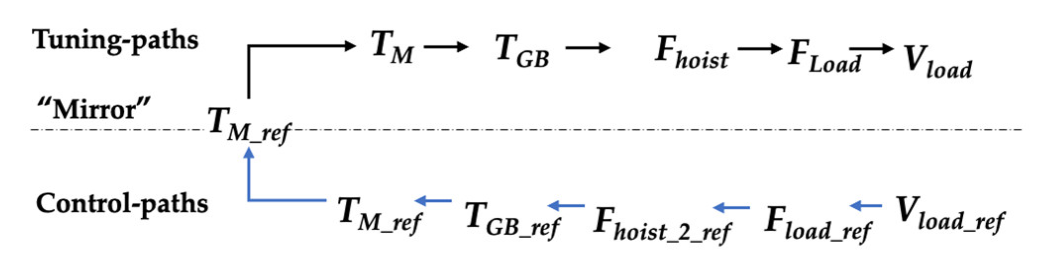
2.5. Port Crane Local Control System

The EMR-based local control system for the traction part of the crane is shown by the blue blocks in Figure 3. EMR formalism is used to obtain the tuning and control paths required for the traction system local control scheme development shown in Figure 4. A tuning path connects the tuning and objective variable, which is the one to be controlled [26]; the control path is the mirror image of the tuning path. For this study, the tuning path is followed from the tuning variable, which is the electrical drive torque $T_{m\_ref}$, to the control variable, which is the load speed $V_{Load}$. The local control system for the crane hoist system is then systematically obtained by the inversion of each of the subsystems [29].

Similarly, by following the tuning path from tuning variable $T_{m\_t\_ref}$ to the control variable $V_{Load\_t}$, the local control system for the crane trolley system is obtained.

Table 3. Modeling the port crane local control system.

	Hoist Local Control System
Gearbox	$T_{m\_ref}=\frac{T_{GB\_ref}}{i_{gb}{\eta }_{gb}^{\gamma }}\left\{ \begin{array}{c}\gamma =1 T_m{\omega }_m \ge 0\\ \gamma =-1 T_m{\omega }_m \ge 0\end{array}\right.$	(20)
Cable drum	$T_{GB\_ref}=F_{hoist\_ref}\times r_{drum}$	(21)
Spreader	$F_{hoist\_ref}=F_{L\_ref}/4$	(22)
Load	$F_{L\_ref}=C_{load}\left(s\right)\left(V_{L\_ref}-V_L\right)+F_{res}$	(23)
	Trolley Local Control System
Gearbox	$T_{m\_t\_ref}=\frac{T_{GB\_t\_ref}}{i_{gb\_t}{\eta }_{gb\_t}^{\gamma }}\left\{ \begin{array}{c}\gamma =1 T_{m\_t}{\omega }_{m\_t} \ge 0\\ \gamma =-1 T_{m\_t}{\omega }_{m\_t} \ge 0\end{array}\right.$	(24)
Wheel	$T_{GB\_t\_ref}=F_{load\_t\_ref}\times R_{wheel}$	(25)
Load	$F_{L\_ref}=C_{load}\left(s\right)\left(V_{L\_ref}-V_L\right)+F_{res}$	(26)

provides the mathematical equations used to model the port crane control system. Except for the load, for all other mechanical transmission systems, the local control system is obtained via direct inversion of their mathematical equations, as shown in Equations (20)–(22), (24), and (25). Indirect inversion of the load is modeled in Equations (23) and (26), where a closed-loop proportional–integral (PI) controller $C_{load}\left(s\right)$ is used in a closed loop. The PI controller outputs $F_{L\_ref}$ and inputs the measured load speed $V_L$, disturbance $F_{res}$, and a reference crane hoist speed profile $V_{L\_ref}$.

3. Development of the Optimal Port Crane Trajectory

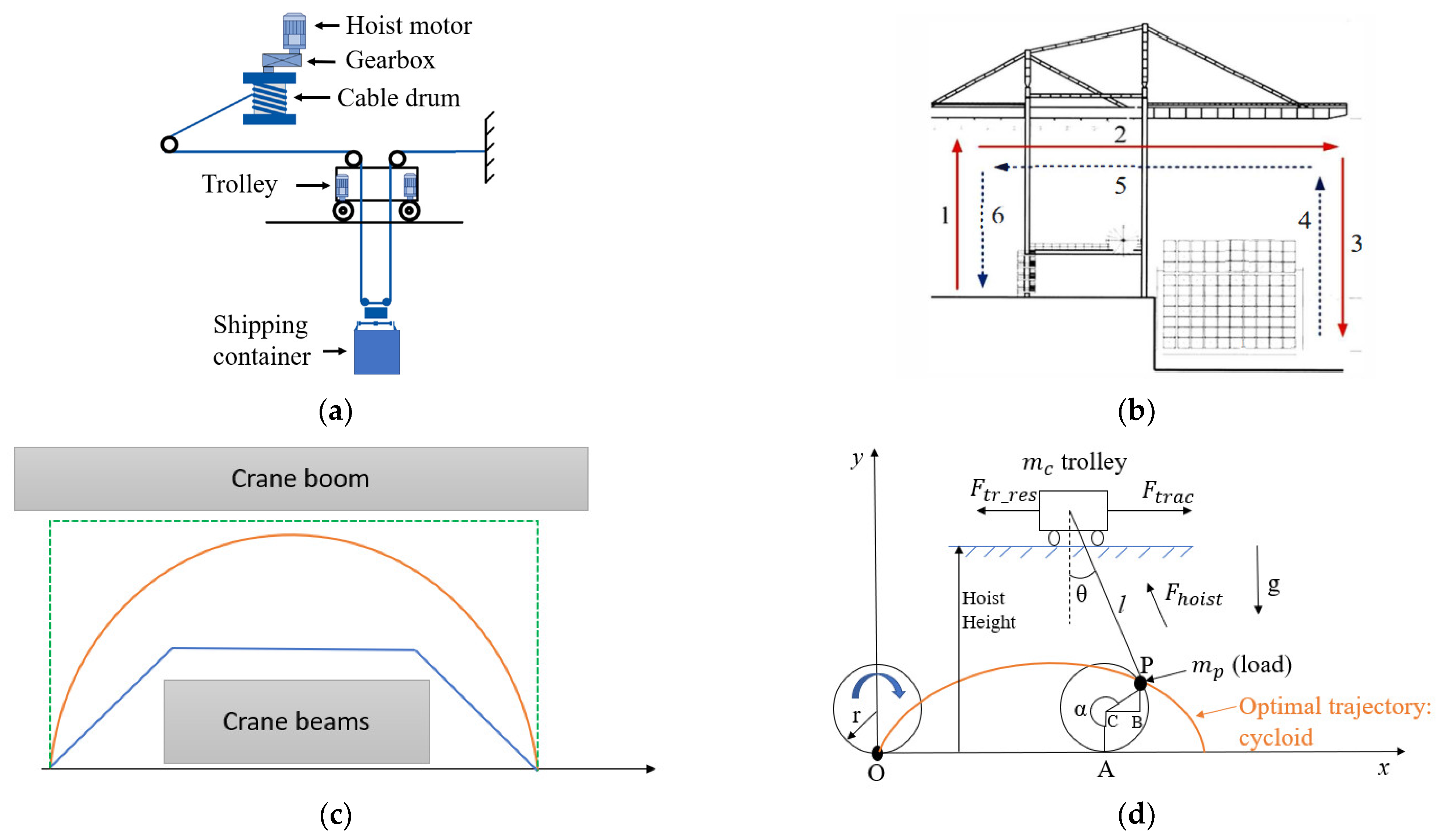
3.1. Description of the Port Crane Load-Handling Mechanism

Figure 5a shows the port crane load-handling mechanism, which consists of the load hoisting system and the crane’s trolley. When handling shipping container loads, the STS crane makes the three motions shown in Figure 5b; these are the trolley motion horizontally and both the hoisting and lowering motions vertically. The crane also moves sideways along the ship in what is called the gantry motion, but this is undertaken without load and the trolley, hoisting, and lowering motions. The port crane load-handling trajectory, therefore, consists only of the trolley and hoist motions. Figure 5a shows that the crane’s load is suspended under the trolley, which moves between the ship and the shore. Steel wire ropes are used to hoist and lower the load under the trolley; the load is hooked onto the crane’s spreader. The result of the hoisting and the trolley motions is a path along which the load travels between the ship and the shore.

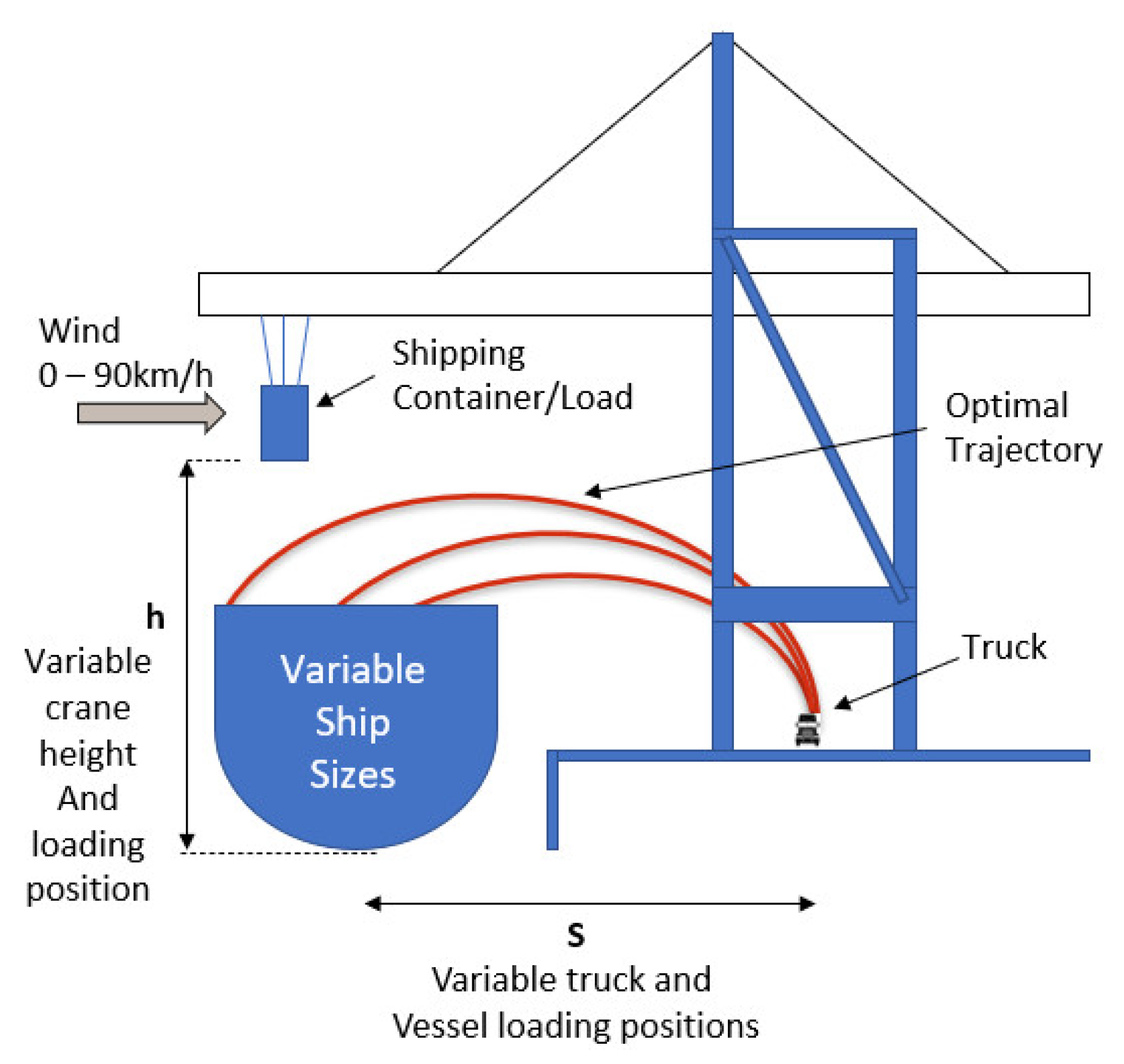
3.2. Optimal Port Crane Trajectory

The crane’s hoisting motions and mechanism in Figure 5b are deduced in Figure 5c into three possible trajectories the crane can follow; the three trajectories and any other path in between represent the space within which lies the crane’s optimal trajectory. The crane’s boom and bottom structure are the limits within which the crane load moves between the ship and the shore. Ports measure productivity in terms of the number of containers the crane loads per hour, also called moves per hour [20]. Therefore, the optimal trajectory for the port crane is the one that minimizes the time it takes the crane to move a container between the ship and the shore.

It is observed that the port crane optimal trajectory problem resembles a combination of the cart–pendulum and the brachistochrone problems, which may be solved using the Lagrangian mechanics approach. The brachistochrone problem was solved in the 1600s by Bernoulli, Newton, and others [30]. The port crane forms a special case where the brachistochrone curve is inverted and the force acting on the thread is the resultant force between the gravitational and crane motor acceleration forces. The brachistochrone is the fastest path for a bead to roll down a frictionless wire joining two points under gravity. The brachistochrone is a segment of a cycloid, which is the curve traced out by a point on the rim of a circular wheel or circle rolling in a straight line. In the case of a port crane, the bead represents the shipping container. The optimal trajectory for the crane load with the shortest time between ship and shore is, therefore, cycloid (Figure 5d). In [31], it is shown that the brachistochrone curve observes the principle of stationary action. This property of the brachistochrone curve is applicable to the port crane optimal trajectory problem as the crane’s motion starts and ends at stationary points. Figure 5d shows a classical mechanics model of the port crane. The cart–pendulum approach is used to represent the trolley with a suspended load and is useful for modeling the load sway problem. The load sway problem has been well studied, as shown in [32], and it is not the focus of this study. In practice, the load sway is minimal with θ being very small because of a much faster anti-sway control system and heavy crane load. The optimal crane trajectory is therefore found by solving the brachistochrone problem.

The brachistochrone problem is about determining the shape of the curve along which a bead, starting from a state of rest and subject to gravitational acceleration, will travel between two points, $P_1$ and $P_2$, in the shortest time possible without any friction. The time to travel between the two points is given the integral:

$$t_{12}={{\displaystyle \int }}_{P_2}^{P_1}\frac{ds}{v}$$

(27)

where $s$ is the arc length, and $v$ is the speed; the speed at any point along the curve is given by applying the principle of conservation of energy and equating kinetic energy to gravitational potential energy, as follows:

$$\frac{1}{2}m{v}^2=mgy$$

(28)

which gives:

$$v=\sqrt{2gy}$$

(29)

Substituting Equation (29) into (27), together with the identity:

$$ds=\sqrt{d{x}^2+d{y}^2}=\sqrt{1+y^{{\prime }^2}}dx$$

(30)

This gives the functional of the brachistochrone:

$$t_{12}={{\displaystyle \int }}_{P_2}^{P_1}\sqrt{\frac{1+y^{{\prime }^2}}{2gy}}dx$$

(31)

Given that the rolling bead is starting from a stationary position in an $xy$plane, the coordinates of the two points are then $P_1=\left(0, 0\right)$and $P_2=\left(\mathrm{b},\mathrm{B}\right)$. Then, the functional of the brachistochrone with its boundary conditions is given by:

$$T\left[y\right]=\frac{1}{\sqrt{2g}}{{\displaystyle \int }}_0^b\sqrt{\frac{1+{\left(y^{\prime }\right)}^2}{y}}dx, y\left(0\right)=0, y\left(b\right)=B$$

(32)

The function to be varied is thus:

$$f=\sqrt{\frac{1+{\left(y^{\prime }\right)}^2}{2gy}}$$

(33)

The function $f\left(y,y^{\prime }\right)$ is independent of x; therefore, $\frac{\partial f}{\partial x}=0$. The Beltrami identity, which is the special case of the Euler–Lagrange method, is therefore used to find the extremum:

$$y^{\prime } \frac{\partial f}{\partial y^{\prime }}-f=C$$

(34)

Then:

$$\frac{\partial f}{\partial y^{\prime }}=y^{\prime } {\left(1+{\left(y^{\prime }\right)}^2\right)}^{-1/2}{\left(2gy\right)}^{-1/2}$$

(35)

Substituting Equations (35) and (33) into (34) gives:

$$\frac{1}{\sqrt{2gy}\sqrt{1+{\left(y^{\prime }\right)}^2}}=C$$

(36)

By squaring and rearranging Equation (36), this gives:

$$\left(1+{\left(\frac{dy}{dx}\right)}^2\right)y=\frac{1}{2g{C}^2}$$

(37)

$$\left(1+{\left(\frac{dy}{dx}\right)}^2\right)y=k^2$$

(38)

In Equation (39), the square of the old constant $C$is expressed by a new positive constant $k^2$. The solution to this equation is then given by the parametric equations:

$$x=\frac{1}{2}{k}^2\left(2\alpha -\sin 2\alpha \right)$$

(39)

$$y=\frac{1}{2}{k}^2\left(1-\cos 2\alpha \right)$$

(40)

Equations (39) and (40) are those of a cycloid. Furthermore, it has been shown in Equation [33] that the brachistochrone problem can be extended to include friction. This yields the parametric solutions:

$$x=\frac{1}{2}{k}^2\left[\left(\alpha -\sin \alpha \right)+\mu \left(\alpha -\cos \alpha \right)\right]$$

(41)

$$y=\frac{1}{2}{k}^2\left[\left(1-\cos \alpha \right)+\mu \left(\alpha +\sin \alpha \right)\right]$$

(42)

In the case of a port crane energy management study, the friction force is negligible compared to the crane motor’s acceleration and gravitational forces. The optimal trajectory for port cranes is therefore a cycloid and is given by Equations (43) and (44) as follows:

$$x=r\left(\alpha -\sin \alpha \right)$$

(43)

$$y=r\left(1-\cos \alpha \right)$$

(44)

The constant $\frac{1}{2}{k}^2$ has been substituted using trigonometry with the radius $r$ of the rolling circle that creates the cycloid curve.

The optimal crane hoist/vertical and trolley/horizontal speed profiles are obtained from the derivatives of Equations (43) and (44) as follows:

$$V_x=V\_trolley=r\left(1-\cos \alpha \right)$$

(45)

$$V_y=V\_hoist=r\sin \alpha$$

(46)

where the radius of the rolling circle r is deduced from the crane height, ship size, and container loading position, and the parameter α corresponds to the rotational angle of the rolling circle as the crane trolley moves horizontally between the ship and shore.

Based on the brachistochrone problem, the time it takes for the shipping container to travel along the cycloid path between ship and shore is given by Equation (47). In the traditional brachistochrone problem where a frictionless surface is assumed, the acceleration $a$ equals gravitational acceleration; however, in the crane application, the resultant acceleration is obtained from the crane’s motor design parameters based on the balance of forces required to hoist the shipping container. The relationship between the rotational angle α and travelling time is given by Equation (36).

$$t=2\pi \sqrt{r/a}$$

(47)

$$\alpha \left(t\right)=t\sqrt{a/r}$$

(48)

The relationship in Equation (48) shows that as α increases from 0 to 2$\pi$, the optimal time it takes for the crane to move a shipping container between ship and shore is dependent on the radius of the rolling circle.

The radius of the rolling circle is given by the height to which the load is hoisted to clear crane beams and the distance from the truck on shore to the loading position in the ship. The crane height and ship-to-shore distance vary because of various ship sizes and port crane sizes. There is further variation in container loading position because of the multiple container loading slots on the ship and the multiple truck lanes on shore. Port cranes’ performance and energy consumption are highly impacted by wind; 90 km/h is the maximum wind speed at which cranes operate. The variation in container loading positions, crane height, ship sizes, and wind speed results in multiple optimal cycloid load trajectories for port cranes, as shown in Figure 6. The multiple optimal crane trajectories result in multiple optimal power consumption curves. The particle swarm optimization technique is then selected to find the set of optimal crane trajectories and their associated optimal crane energy consumption because of PSO’s ability to solve optimization problems with multiple objectives and parameters.

3.3. Port Crane Optimal Power Consumption

This section uses the PSO algorithm and the optimal trajectory above to find the optimal power and energy consumption for port cranes.

PSO’s inputs are mainly algorithm-specific hyper-parameters. The user input consists of the objective function, also called the fitness function. In the PSO algorithm, the fitness or objective function serves as the criterion for performance evaluation; usually defined through a mathematical formula, the performance criterion quantifies the achieved system performance through a performance index [34].

For the port crane power optimization problem, the PSO algorithm’s fitness is developed in Equations (49)–(56). The power consumed by the port crane is given by Equation (49) and consists of the power used by the crane motors when conducting hoisting and trolley motions. Equation (50) expresses the power consumption in terms of the speeds and forces required by the hoisting and trolley motions.

$$P_{grid}=P_{crane\_load}=P_{hoisting\_motion}+P_{trolley\_motion}$$

(49)

$$P_{grid}=F_{hoist}{V}_{hoist}+F_{trolley}{V}_{trolley}$$

(50)

The complete grid power consumption equation is then obtained by substituting Equations (12) and (19) into (50) as follows:

$$P_{grid}=\frac{\left(M_{L}g+0.5\rho c_{x}A{(V_{hoist}+V_{wind})}^2\right)V_{hoist}}{{\eta }_{ED}{\eta }_{GB}}+\frac{\left(M_{L+tr}\left(g+fg\right)+0.5\rho c_{x}A{(V_{trolley}+V_{wind})}^2\right)V_{trolley}}{{\eta }_{ED\_tr}{\eta }_{GB\_tr}}$$

(51)

The port crane energy consumption, Equation (52), is used as the fitness function in the PSO algorithm, and it is therefore the objective function for the optimization problem.

$$E_{grid}\left(V_{trolley},V_{hoist},V_{wind}\right)=P_{grid}\left(V_{trolley},V_{hoist},V_{wind}\right)\times t$$

(52)

The PSO algorithm’s fitness function in Equation (52) has the following constraints:

$$0 \le V_{hoist}\le V_{hoist\_max}$$

(53)

$$0 \le V_{trolley}\le V_{trolley\_max}$$

(54)

$$0 \le V_{wind}\le V_{wind\_max}$$

(55)

$$0 \le P_{grid}\le P_{grid\_max}$$

(56)

The optimization parameters for the PSO simulation are the wind speed, the crane load’s horizontal speed, and the crane load’s vertical speed. The crane load’s velocities $V_{hoist}$ and $V_{trolley}$ are obtained from Equations (45) and (46). These equations have two variables, which are the load acceleration $a$ and the radius $r$, which describes the crane lifting height and ship-to-shore distance. Practical constraints to the optimization parameters have been considered in simulations. These include the crane lifting height not exceeding 35 m, wind speed not exceeding 25 m/s, load horizontal speed not exceeding 4 m/s, and load vertical speed not exceeding 3 m/s. The result of the PSO algorithm simulation is a set of optimal power consumption curves.

The PSO algorithm is best described by its mathematical model, which consists of the current particle position and its velocity vector. The current particle position is calculated by:

$$\overrightarrow{X_i^{t+1}}=\overrightarrow{X_i^t}+\overrightarrow{V_i^{t+1}}$$

(57)

The velocity of the particle position is calculated by:

$$\overrightarrow{V_i^{t+1}}=w\overrightarrow{V_i^t}+c_1{r}_1\left(\overrightarrow{P_i^t}-\overrightarrow{X_i^t}\right)+c_2{r}_2\left(\overrightarrow{G^t}-\overrightarrow{X_i^t}\right)$$

(58)

The pseudo-code of PSO Algorithm 1 is shown below [35]:

Algorithm 1. PSO pseudo-code.

Initialize $\mathrm{the} \mathrm{optimization} \mathrm{problem} \mathrm{parameters} (V_{hoist}$, $V_{trolley}$, $V_{wind})$ $$\begin{gathered} \mathbf{Initialize} \mathrm{the} \mathrm{limits} \mathrm{of} \mathrm{the} \mathrm{optimization} \mathrm{parameters} \mathrm{from} \mathrm{Equations} \left(53\right)–\left(55\right) \\ \hspace{1em}\hspace{1em}0 \le V_{hoist}\le 3 \mathrm{m}/\mathrm{s} \\ \hspace{1em}\hspace{1em}0 \le V_{trolley}\le 4 \mathrm{m}/\mathrm{s} \\ \hspace{1em}\hspace{1em}0 \le V_{wind}\le 25 \mathrm{m}/\mathrm{s} \end{gathered}$$ Initialize the PSO hyper-parameters (N, c1, c2, Wmin, Wmax, Vmax, and MaxIter) Initialize the population of N particles   do   for each particle     calculate the objective or fitness of the particle using Equation (52)     Update PBEST if required     Update GBEST if required   end for   Update the inertia weight   for each particle   Update the velocity (V)   Update the position (X)   end for while the end condition is not satisfied Return GBEST as the best estimation of the global optimum

4. Experimental Validation

4.1. Experimental Setup

The crane’s EMR model was validated using the power consumption and hoist motor speed data recorded from a real-world STS crane at the Cape Town Container Terminal. The experimental setup is shown in Figure 7a,b; a Fluke 1736 power logger was used to record the crane’s actual power consumption when loading and unloading shipping containers. The power recordings were undertaken at the 500 kW hoist motors, which are the main power consumers, and at the low-voltage (LV) panel, which is the crane’s main supply. The hall effect sensor mounted close to a magnet on the shaft of the hoist motor was used to measure the speed of the hoist motor shaft. The speed measurement was undertaken by processing the hall effect sensor output with an Arduino Uno board and a laptop running MATLAB/Simulink. The crane was carrying a 20 t load during the experiment.

Real-world cranes are designed to handle their loads using a predetermined speed reference curve, as shown in Figure 8a; this trapezoidal-shaped speed setpoint curve consists of an initial acceleration of the crane hoist motor when lifting the load and, then, a constant speed phase. This is followed by a deceleration phase when arriving at the load destination; the final stage is that of lowering the load into its final landing position. The final stage of lowering the container load results in the production of regenerative braking energy by the crane hoist motors; this energy is burnt in the braking resistor.

Using the trapezoidal-shaped speed setpoint curve for the crane motors results in a nonoptimal trapezoidal-shaped power consumption trajectory for the port crane. The real-world recorded motor speed from the crane is used as the input speed $V_{Load\_ref}$ in Figure 3 for the MATLAB/Simulink simulation; the simulated hoist motor power consumption is then compared with the real-world hoist motor power consumption recorded from the crane for validation.

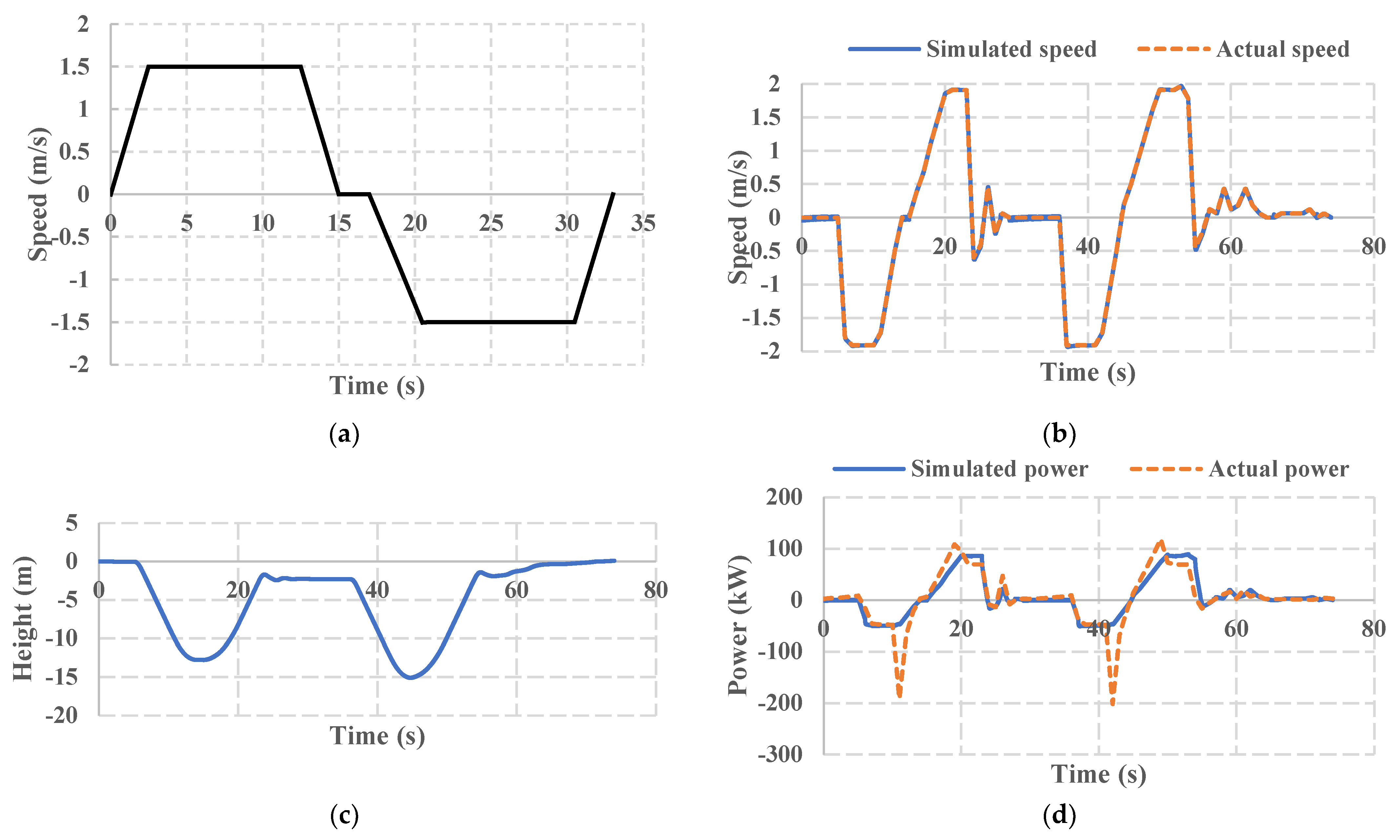
4.2. Experimental Results

Figure 8b shows that the simulated load hoisting speed is the same as that of the real-world crane. Figure 8c shows the load hoisting trajectory, which is nonoptimal because of the trapezoidal-shaped reference speed curve; the load hoisting trajectory is obtained by taking a derivative of the real-world speed. The trajectory is inverted because the load-handling spreader was suspended at height when the crane began its operation; this is the normal resting position for the crane driver. Figure 8d shows that the crane’s EMR simulation model power consumption closely matches that of a real-world crane. However, the real-world crane power consumption curve is more dynamic compared to the simulated crane curve.

It has been shown in [27,28] that, for energy management studies, it is appropriate to reduce the fast dynamical crane components to their static models; this is because the energy management strategy lies higher than the crane’s control system, which requires a fast dynamic model.

The highly dynamical real-world crane power consumption curve is caused by human drivers and the crane’s control system. It is noted that a solution to the real-world crane’s dynamical power consumption curve is in the automation of port cranes and the utilization of optimal sinusoidal speed setpoint curves.

Based on the results above, it is therefore confirmed that the EMR-based simulation model appropriately represents the actual crane power consumption.

The focus of this study is on energy saving, and therefore, only the positive half cycle of the crane power consumption curve is considered when the crane motors are consuming energy from the grid; the regenerative braking energy is not considered as it is burnt in the braking resistor.

5. Optimal vs. Nonoptimal Trajectory

This section compares the optimal cycloid port crane trajectory with the traditional trapezoidal-shaped nonoptimal load trajectory. As discussed above, ports measure productivity in terms of the number of containers lifted by the port crane per hour, i.e., frequency “f” [20]. The more the crane container moves per hour, the quicker the vessel turnaround time at the port; [20] shows that port cranes make between 30 and 60 moves per hour. The duration taken by the crane to lift and move a container between ship and shore is therefore given by:

$$T=1/f$$

(59)

Port cranes have a dwell time of 30 s [20]; this is the time taken by the crane’s starting and stopping motions, finding the correct spot on the truck and vessel, and checking for clearances. The duration T, therefore, consists of the 30 s dwell time and the actual container moving time. The real-world crane in this study has an average loading duration of 33 s, excluding the dwell time; the loading duration, therefore, becomes 63 s when the 30 s dwell time is included.

Figure 9 shows the average crane moves per hour in 2021 of port cranes around the world [36]; the average maximum performance was 24.2 moves per hour on ships carrying between 13,500 and 80,501 shipping containers. Using Equation (59), the optimal trajectory load cycle duration is calculated in

Table 4. Optimal Trajectory Load Cycle Duration.

Ship-to-Shore Distance (m)	Min.	Avg.	Max.
	20	50	100
Cycloid radius, i.e., half crane lifting height (m)	3.2	8.0	15.9
Actual crane moving time (s)	9.8	15.5	21.9
Dwell time (s)	30	30	30
Total duration of crane move (s)	39.8	45.5	51.9

. The real-world crane dimensions are used to determine the minimum, average, and maximum container loading distances between the ship and truck on shore, which are 20 m, 50 m, and 100 m, respectively.

The real-world crane hoisting gear lifting height is used to determine the optimal cycloid trajectory radius. The calculation results show that a crane following an optimal load trajectory will have a load cycle duration of between 39.8 s and 51.9 s. Figure 10a compares the optimal and nonoptimal crane load trajectories along the crane productivity curve. The crane productivity curve is developed using the typical crane performance data from [20]. Based on the crane load duration of 63 s and 45.5 s for the optimal and nonoptimal crane load trajectories, respectively, the resultant crane productivity of 79 and 57 moves per hour for the optimal and nonoptimal load trajectories are obtained by Equation (59). The faster load-handling time and the higher number of moves per hour result in the optimal crane load trajectory being 38.59% faster and more productive than the nonoptimal crane load trajectory.

Figure 10b shows that when compared to the nonoptimal trajectory, the optimal trajectory has a smooth shape and requires less time and lifting height to complete the crane move.

6. Simulation Results

This section presents the MATLAB simulation results. First, the particle swarm optimization algorithm is used to find the set of pareto optimal crane trajectories given the variation in crane size, ship size, and wind speed. The crane’s optimal power consumption from the grid in Equation (37) is used as the objective function in the PSO simulation. The results of the PSO simulation is a set of pareto optimal crane trajectories shown in Figure 11a. Each of the 500 dots in Figure 11a represents a crane’s optimal cycloid trajectory, as illustrated in Figure 6. Figure 11b shows the corresponding optimal energy consumption for each of the 500 pareto optimal crane trajectories.

The set of pareto optimal solutions in Figure 11a represents a general guideline for crane designers. The guideline in Figure 11a,b allows crane designers to select a crane based on its energy consumption, then obtain its corresponding crane size and maximum wind speed limit. This process can also be conducted in reverse by providing crane size and wind speed parameters to obtain the crane’s optimal energy consumption. The boundary condition for wind in Figure 11a is based on port cranes not operating beyond a 90 km/h wind speed, which is gale-force wind. The maximum lifting height of 35 m is based on current maximum container ship sizes; there is no limitation to crane designers increasing this parameter. The mean energy consumption of the optimal trajectory is 2.25 kWh, and the maximum is 9.17 kWh.

The MATLAB Simulink EMR library was then used for software simulation of the port crane EMR-based model shown in Figure 3. This simulation compares a real-world crane to an optimal trajectory-based crane obtained using the real-world crane parameters in the PSO simulation above.

Figure 11c,d show the simulation results. The optimal trajectory reduces the cranes’ peak power consumption by 36.38% when compared with the nonoptimal trajectory. As shown in Figure 11d, the crane on an optimal trajectory consumes 1.98 kWh per load cycle; this is a 36.40% reduction in energy consumption compared to the 2.70 kWh consumed by cranes following a nonoptimal trajectory. The optimal trajectory consumes 12% less energy compared to an experienced crane driver.

The optimal trajectory has a faster load-handling time of 30 s compared to the 35 s and 40 s for the nonoptimal trajectory.

Furthermore, the smooth sinusoidal crane power consumption curve confirms the need for the automation of port cranes to reduce the dynamical crane power consumption caused by nonoptimal trajectories and human drivers.

7. Conclusions

This paper developed an EMR model of the port crane and the port crane’s optimal load trajectory. The optimal port crane load trajectory obtained in this paper for port cranes is found to be a cycloid path. The outcome of the work can be summarized as follows:

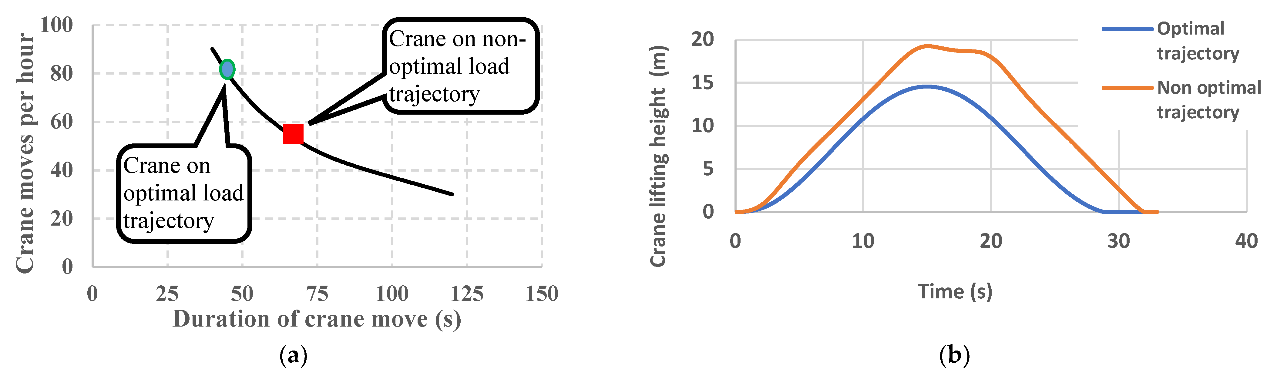
• The developed optimal crane load trajectory is 38.59% faster and more productive than the nonoptimal crane load trajectory;
• The optimal trajectory reduces the cranes’ peak power consumption by 36.38% when compared with the nonoptimal trajectory;
• The optimal trajectory reduces the cranes’ energy consumption by 36.40% and 12% when compared with the nonoptimal and experienced crane driver trajectories, respectively;
• The sinusoidal speed reference curves produced by the cycloid trajectory can be used as a guide for the automated port crane system;
• The outcome of this work will also serve as a guideline for port crane designers in the selection of port cranes based on the required energy consumption, maximum wind speed capability, crane lifting height, and trolley distance between ship and shore.

References

1. Song, D. A Literature Review, Container Shipping Supply Chain: Planning Problems and Research Opportunities. Logistics 2021, 5, 41. [Google Scholar] [CrossRef]
2. Iris, Ç.; Lam, J.S.L. A Review of Energy Efficiency in Ports: Operational Strategies, Technologies and Energy Management Systems. Renew. Sustain. Energy Rev. 2019, 112, 170–182. [Google Scholar] [CrossRef]
3. Zhao, N.; Schofield, N.; Niu, W. Energy Storage System for a Port Crane Hybrid Power-Train. IEEE Trans. Transp. Electrif. 2016, 2, 480–492. [Google Scholar] [CrossRef]
4. Corral-Vega, P.J.; García-Trivi, P.; Fern Andez-Ramírez, L.M. Design, Modelling, Control and Techno-Economic Evaluation of a Fuel Cell/Supercapacitors Powered Container Crane. Energy 2019, 186, 115863. [Google Scholar] [CrossRef]
5. Nguyễn, B.H.; Vo-Duy, T.; Henggeler Antunes, C.; Trovão, J.P.F. Multi-Objective Benchmark for Energy Management of Dual-Source Electric Vehicles: An Optimal Control Approach. Energy 2021, 223, 119857. [Google Scholar] [CrossRef]
6. Nguyen, B. Energy Management Strategies of Electric and Hybrid Vehicles Supplied by Hybrid Energy Storage Systems. Ph.D. Thesis, Faculté de Génie, Université de Sherbrooke, Sherbrooke, QC, Canada, 2019. [Google Scholar]
7. Nguyen, B.H.; German, R.; Trovao, J.P.F.; Bouscayrol, A. Real-Time Energy Management of Battery/Supercapacitor Electric Vehicles Based on an Adaptation of Pontryagin’s Minimum Principle. IEEE Trans. Veh. Technol. 2019, 68, 203–212. [Google Scholar] [CrossRef]
8. Zhao, N. Modelling and Design of Electric Machines and Associated Components for More Electric Vehicles. Ph.D. Thesis, School of Graduate Studies, McMaster University, Hamilton, ON, Canada, 2017. [Google Scholar]
9. Zhou, W.; Cleaver, C.J.; Dunant, C.F.; Allwood, J.M.; Lin, J. Cost, Range Anxiety and Future Electricity Supply: A Review of How Today’s Technology Trends May Influence the Future Uptake of BEVs. Renew. Sustain. Energy Rev. 2023, 173, 113074. [Google Scholar] [CrossRef]
10. Kim, S.M.; Sul, S.K. Control of Rubber Tyred Gantry Crane with Energy Storage Based on Supercapacitor Bank. IEEE Trans. Power Electron. 2006, 21, 1420–1427. [Google Scholar] [CrossRef]
11. Yin, J.; Peng, X.; He, J.; Huo, Q.; Wei, T. Energy Management Method of a Hybrid Energy Storage System Combined with the Transportation-Electricity Coupling Characteristics of Ports. IEEE Trans. Intell. Transp. Syst. 2023, 1–16. [Google Scholar] [CrossRef]
12. Kermani, M.; Parise, G.; Martirano, L.; Parise, L.; Chavdarian, B. Utilization of Regenerative Energy by Ultracapacitor Sizing for Peak Shaving in STS Crane. In Proceedings of the 2019 IEEE International Conference on Environment and Electrical Engineering and 2019 IEEE Industrial and Commercial Power Systems Europe, EEEIC/I and CPS Europe 2019, Genova, Italy, 11–14 June 2019. [Google Scholar]
13. Parise, G.; Honorati, A.; Parise, L.; Martirano, L. Near Zero Energy Load Systems: The Special Case of Port Cranes. In Proceedings of the 2015 IEEE/IAS 51st Industrial and Commercial Power Systems Technical Conference, I and CPS 2015, Calgary, AB, Canada, 5–8 May 2015. [Google Scholar]
14. Vichos, E.; Sifakis, N.; Tsoutsos, T. Challenges of Integrating Hydrogen Energy Storage Systems into Nearly Zero-Energy Ports. Energy 2022, 241, 122878. [Google Scholar] [CrossRef]
15. Kermani, M.; Parise, G.; Martirano, L.; Parise, L.; Chavdarian, B. Power Balancing in STS Group Cranes with Flywheel Energy Storage Based on DSM Strategy. In Proceedings of the 2018 IEEE 59th Annual International Scientific Conference on Power and Electrical Engineering of Riga Technical University, RTUCON 2018, Riga, Latvia, 12–13 November 2018. [Google Scholar]
16. Takalani, R.; Masisi, L. Development of An Energy Management Strategy for Port Cranes. In Proceedings of the IECON Proceedings (Industrial Electronics Conference), Toronto, ON, Canada, 13–16 October 2021. [Google Scholar]
17. Wu, Z.; Xia, X. Optimal Motion Planning for Overhead Cranes. IET Control Theory Appl. 2014, 8, 1833–1842. [Google Scholar] [CrossRef]
18. Wang, X.; Liu, J.; Dong, X.; Peng, H.; Li, C. An Energy-Time Optimal Autonomous Motion Control Framework for Overhead Cranes in the Presence of Obstacles. Proc. Inst. Mech. Eng. Part C J. Mech. Eng. Sci. 2020, 235, 2373–2385. [Google Scholar] [CrossRef]
19. Zhang, W.; Chen, H.; Chen, H.; Liu, W. A Time Optimal Trajectory Planning Method for Double-Pendulum Crane Systems with Obstacle Avoidance. IEEE Access 2021, 9, 13022–13030. [Google Scholar] [CrossRef]
20. Zrnić, N.; Petković, Z.; Bošnjak, S. Automation of Ship-to-Shore Container Cranes: A Review of State-of-the-Art. FME Trans. 2005, 33, 111–121. [Google Scholar]
21. Böck, M.; Stöger, A.; Kugi, A. Efficient Generation of Fast Trajectories for Gantry Cranes with Constraints. IFAC PapersOnLine 2017, 50, 1937–1943. [Google Scholar] [CrossRef]
22. Masih-Tehrani, M.; Ha’iri-Yazdi, M.; Esfahanian, V.; Safae, A. Optimum Sizing and Optimum Energy Management of a Hybrid Energy Storage System for Lithium Battery Life Improvement. J. Power Sources 2013, 244, 2–10. [Google Scholar] [CrossRef]
23. Nguyen, B.H.; Vo-Duy, T.; Ta, M.C.; Trovao, J.P.F. Optimal Energy Management of Hybrid Storage Systems Using an Alternative Approach of Pontryagin’s Minimum Principle. IEEE Trans. Transp. Electrif. 2021, 7, 2224–2237. [Google Scholar] [CrossRef]
24. Sun, X.; Fu, J.; Yang, H.; Xie, M.; Liu, J. An Energy Management Strategy for Plug-in Hybrid Electric Vehicles Based on Deep Learning and Improved Model Predictive Control. Energy 2023, 269, 126772. [Google Scholar] [CrossRef]
25. Bouscayrol, A.; Davat, B.; De Fornel, B.; Francois, B.; Hautier, J.P.; Meibody-Tabar, F.; Pietrzak-David, M. Multi-Converter Multi-Machine Systems: Application for Electromechanical Drives. Eur. Phys. J. Appl. Phys. 2020, 10, 131–147. [Google Scholar] [CrossRef]
26. Bouscayrol, A.; Hautier, J.P.; Lemaire-Semail, B. Graphic Formalisms for the Control of Multi-Physical Energetic Systems: COG and EMR. In Systemic Design Methodologies for Electrical Energy Systems: Analysis, Synthesis and Management; John Wiley and Sons: Hoboken, NJ, USA, 2013; pp. 89–124. ISBN 9781848213883. [Google Scholar]
27. Castaings, A.; Lhomme, W.; Trigui, R.; Bouscayrol, A. Comparison of Energy Management Strategies of a Battery/Supercapacitors System for Electric Vehicle under Real-Time Constraints. Appl. Energy 2016, 163, 190–200. [Google Scholar] [CrossRef]
28. Nguyên, B.H.; Trovão, J.P.; German, R.; Bouscayrol, A. An Optimal Control-Based Strategy for Energy Management of Electric Vehicles Using Battery/Supercapacitor. In Proceedings of the 2017 IEEE Vehicle Power and Propulsion Conference, VPPC, Belfort, France, 11–14 December 2017; pp. 1–6. [Google Scholar]
29. Lhomme, W.; Bouscayrol, A.; Syed, S.A.; Roy, S.; Gailly, F.; Pape, O. Energy Savings of a Hybrid Truck Using a Ravigneaux Gear Train. IEEE Trans. Veh. Technol. 2017, 66, 8682–8692. [Google Scholar] [CrossRef]
30. Boyer, C.; Merzbach, U. A History of Mathematics; John Wiley & Sons: Hoboken, NJ, USA, 2011. [Google Scholar]
31. Perlick, V. The Brachistochrone Problem in a Stationary Space-time. J. Math. Phys. 1991, 32, 3148–3157. [Google Scholar] [CrossRef]
32. Sun, N.; Fang, Y.; Zhang, Y.; Ma, B. A Novel Kinematic Coupling-Based Trajectory Planning Method for Overhead Cranes. IEEE/ASME Trans. Mechatron. 2012, 17, 166–173. [Google Scholar] [CrossRef]
33. Ashby, N.; Brittin, W.E.; Love, W.F.; Wyss, W. Brachistochrone with Coulomb Friction. Am. J. Phys. 1975, 43, 902–906. [Google Scholar] [CrossRef]
34. Pedrycz, W.; Sillitti, A.; Succi, G. Computational Intelligence: An Introduction. Stud. Comput. Intell. 2016, 617, 13–31. [Google Scholar] [CrossRef]
35. Poli, R.; Kennedy, J.; Blackwell, T. Particle Swarm Optimization: An Overview. Swarm Intell. 2007, 1, 33–57. [Google Scholar] [CrossRef]
36. The World Bank. Transport Global Practice: The Container Port Performance Index 2021: A Comparable Assessment of Container Port Performance; The World Bank: Washington, DC, USA, 2021. [Google Scholar]
Figure 1. Overhead crane load-handling trajectory.
Energies 16 07172 g001
Figure 2. Studied port crane system.
Energies 16 07172 g002
Figure 3. Port crane EMR and inversion-based local control.
Energies 16 07172 g003
Figure 4. Port crane local control system.
Energies 16 07172 g004
Figure 5. Port crane hoist and trolley mechanisms layout (a); port crane motions, hoisting (1 & 4), lowering (6 & 3), and trolley (2 & 5) (b); port crane trajectories and constraints (c); and optimal port crane trajectory (d).
Energies 16 07172 g005
Figure 6. Multiple optimal cycloid port crane load trajectories.
Energies 16 07172 g006
Figure 7. Experimental setup (a,b): (1) hoist motor; (2) Fluke 1736 power logger; (3) cable drum; (4) gearbox; (5) mechanical brakes; (6) PC, Arduino UNO board and hall effect sensor; (7) low-voltage panel.
Energies 16 07172 g007
Figure 8. Port crane (a) hoist motor reference speed profile, (b) simulated vs. actual speed, (c) nonoptimal trajectory, and (d) simulated vs. actual power consumption.
Energies 16 07172 g008
Figure 9. Real-world crane loading frequency per ship size [36].
Energies 16 07172 g009
Figure 10. Optimal vs. nonoptimal crane trajectories: (a) crane productivity curve-based comparison; (b) trajectory-based comparison.
Energies 16 07172 g010
Figure 11. Simulation results: (a) a set of pareto optimal solutions; (b) optimal power consumption trajectories; (c) comparing optimal and nonoptimal crane trajectories’ power consumption; (d) comparing optimal and nonoptimal crane trajectories’ energy consumption.
Energies 16 07172 g011