Numerical Investigation and Optimization of a District-Scale Groundwater Heat Pump System

Abstract

Groundwater heat pump (GWHP) systems are acknowledged as renewable and sustainable energy sources that can effectively fulfill the heating and cooling requirements of buildings on a district level. These systems harness geothermal sources available at shallow depths. To ensure the long-term sustainability of the system, the thermally used water is generally reinjected into the aquifer, creating a thermal plume starting from the injection well. Over time, this thermal plume may reach the abstraction well in the long term, potentially leading to a reduction in system efficiency. The operation types have a significant impact on this matter, and their effects have not been extensively studied in the existing literature. Therefore, this study aims to determine the optimal operating configurations for the Northern Gateway Heat Network, a GWHP system established in Colchester, UK. In this study, four distinct operation types are considered: (1) continuous heating (actual system), (2) heating and recovery, (3) heating and cooling, and (4) aquifer thermal energy storage (ATES). The results indicate that ATES operation yields the highest thermal energy output due to its ability to benefit from stored energy from the previous operation. However, implementing the ATES system may encounter challenges due to factors such as well development, hydraulic conductivity, and hydraulic gradient. On the other hand, implementing heating and cooling operations does not require additional considerations and offers not only free cooling to buildings but also a delay in thermal feedback time.

1. Introduction

A significant part of the overall energy consumption in the world is attributed to meeting the heating and cooling needs of buildings [1]. Considering this reality, coupled with the target of achieving net-zero carbon emissions by 2050, it becomes vital to supply the heating and cooling demand of buildings using renewable energy sources. Extensive research and practical implementations have demonstrated that groundwater heat pump (GWHP) systems have the capacity to provide a significant amount of heating and cooling [2]. Recent developments indicate that utilizing GWHP systems at the district level can enhance efficiency and reduce payback period, thereby increasing economic viability and sustainability of the system [3].

GWHP systems harness geothermal sources found in the shallow depths, where groundwater temperatures are relatively lower compared to deep aquifers. As a result, higher efficiencies, defined as coefficient of performance (COP) for GWHPs, can be achieved when utilized for cooling purposes (ranging between 6 and 8) compared to heating applications (ranging between 4 and 6) [4]. In certain instances where groundwater temperatures are exceptionally low, GWHP systems can even offer free cooling, further enhancing its energy-saving capabilities [5].

The reinjection of thermally altered water into the ground creates a thermal plume that mainly develops around the injection wells [6]. In certain cases, the thermal plume may extend towards the abstraction well, leading to a reduction in system efficiency, especially in the long run [7]. It is crucial to carefully analyze various parameters that impact the thermal plume development, including injection and abstraction rates, well separation, transmissivity, hydraulic gradient, etc. [8]. Another significant factor influencing the system efficiency and sustainability is system operation. Banks [8] highlighted that seasonally balanced systems can maintain sustainable operation with injection of cooler water during winter and warmer water during summer. The literature contains numerous studies focusing on the thermal investigation of ATES systems, revealing that ATES operation not only balances cooling and heating needs but also enhances efficiency by utilizing stored energy in the subsurface [9,10,11,12,13].

Previous studies on the optimization of GWHP systems have primarily focused on parameters such as well distance between injection and abstraction wells [7,8] and well locations and injection/abstraction rates [14,15]. Many studies have been conducted on thermal plume development and its impact on the system efficiency and sustainability [2,7,16,17,18,19]. A common conclusion drawn from these studies is that the thermal plume might affect the system performance, which depends on several factors that need to be considered during the design stage.

While several studies have explored the optimization of GWHPs [3,20,21,22,23], only Blázquez et al. [20] has considered the optimization of a district-level GWHP system. They performed an optimization analysis by considering two scenarios related to the network of heat pumps for a district-level GWHP system to evaluate different configurations and their performance. The results show that the efficiency in the first scenario, which involves a single heat pump covering the total demand, is slightly higher than the second scenario that utilizes three heat pumps. This higher efficiency was attributed to lower energy consumption in the first scenario. Furthermore, the lower total initial investment cost in the first scenario enhances its economic viability.

Previous studies on GWHP thermal investigation have predominantly focused on small- to large-scale systems, primarily examining one or two operating configurations for system optimization. Many of these studies have recommended the use of the ATES system. However, it is important to note that the applicability of the ATES system may be limited due to specific requirements, such as proper well development, low hydraulic gradient, and low hydraulic conductivity.

In this paper, the operation of a GWHP system constructed in Colchester, UK is investigated through numerical modelling. The project, called Northern Gateway Heat Network, was designed solely to supply heating and domestic hot water (DHW) demand at a district level. Due to the continuous heating operation, the thermal plume might affect the system efficiency and sustainability in the long term. Furthermore, the system can supply the cooling need of the district with considerably low electrical input from the heat pump, thanks to the relatively low groundwater temperature (around 12.5 °C). To determine the optimal system operating configurations, four different setups are analyzed: (1) continuous heating (actual system), (2) heating and recovery, (3) heating and cooling, and (4) ATES.

The main novelty of this paper lies in the development of a numerical model that utilizes real data from the case study. Another novelty is that this model is employed to analyze four distinct operating configurations and determine the optimum system configurations in the long term. By doing so, the paper aims to provide valuable insights to designers for developing optimal system configurations.

2. Materials and Methods

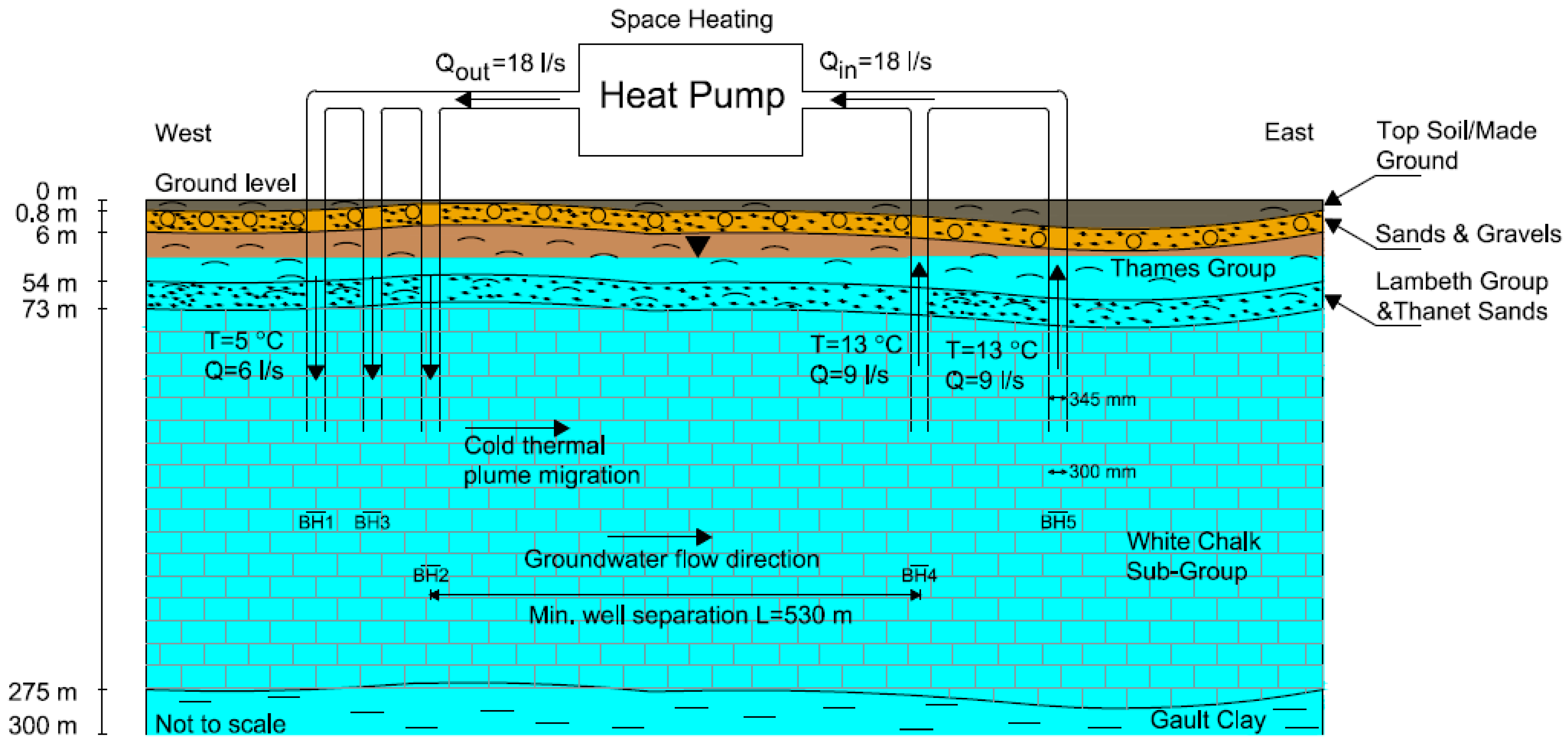
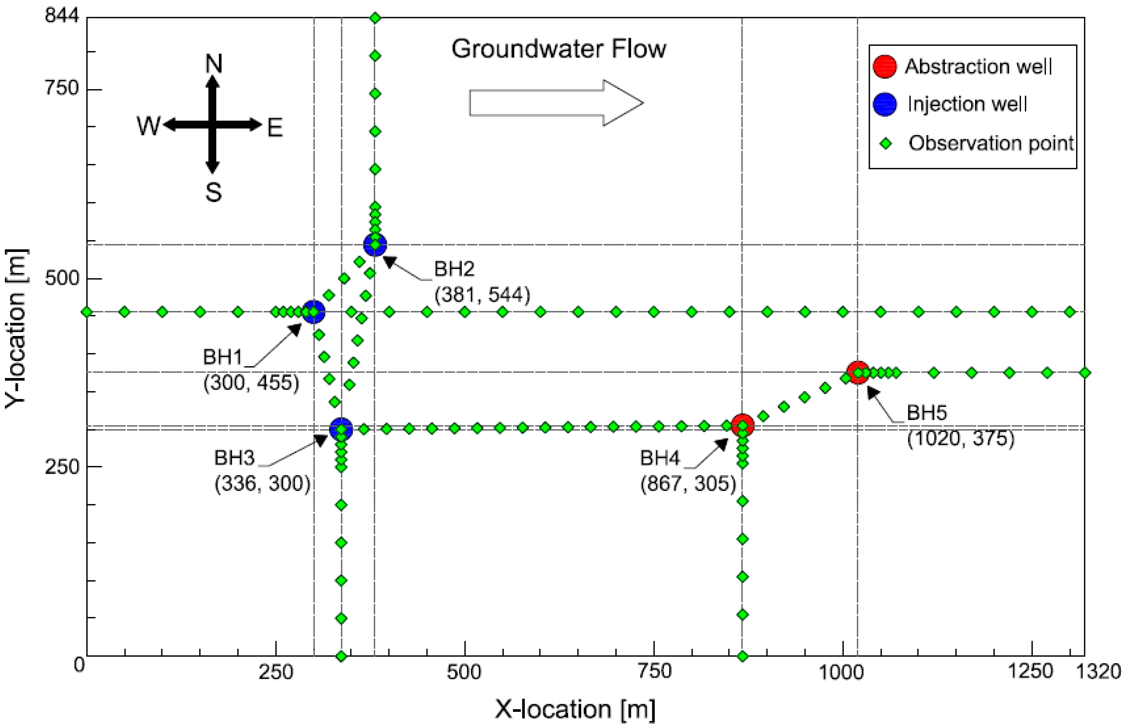
2.1. Site Description

The Northern Gateway Heat Network is a district-level GWHP system using a confined chalk aquifer constructed in Colchester, UK. The project aims to cover 75% of the annual heating and DHW demand of the buildings. Gas boilers are also installed on-site to cover the rest of the demand, particularly during peak loads in winter and as a backup system. The system uses two abstraction and three injection wells drilled to depths of 135 m or 200 m. The water temperature reported by Boon et al. [24] is between 12 °C and 13 °C at the given depths.

The conceptual hydrogeological model of the site, shown in Figure 1, depicts the main geological formations, groundwater flow direction, abstraction and injection well locations, design pumping rates and primary temperatures. With the injection wells positioned up-groundwater gradient from the abstraction wells and potential karstic development, there is a risk of thermal plume migration towards the abstraction wells and reduction in abstracted water temperature over time. This is a key risk for GWHPs, as described by Birks et al. [25]. Therefore, this paper assesses this risk through numerical heat flow modelling.

2.2. Model Description

The model domain was created with dimensions of 1320 m × 844 m × 300 m (length × width × depth), which ensures that flow and heat transfer occurs inside the domain to eliminate edge effects. The locations of the boreholes are shown in Figure 2. The depth of each well was assigned in the simulation using the multilayer well function in FEFLOW based on the information given in Figure 1.

The numbers of elements and nodes are 4,614,796 and 2,337,555, respectively. The observation points were located mainly at 80, 135, and 180 m bgl. Additionally, the observation points were placed at the well surface (i.e., 0 m radial distance), 0.5 and 1 m radial distances from the well surface to observe the temperature profile of the soil.

Observation points were placed at the surface of all wells at depths of 80, 135 and 180 m bgl. They were also located between the wells to observe the interaction between them. Several observation points were placed around the wells at each layer to observe the vertical thermal distribution. The results were also obtained between the surface of each well and the model boundary, as shown in Figure 2.

2.3. Numerical Simulation

A finite element modelling package, FEFLOW, was used to analyze the effect of different operating configurations on the aquifer and its impact on the system sustainability in long-term operation (100 years) for the considered case study. This finite element code is based on mathematical principles of conservation of mass, momentum, and energy for the phases of solid, liquid, and gas, shown in Equations (1)–(3), respectively.

Conservation of mass equation:

$$\frac{\partial }{\partial t}\left({\epsilon }_{\alpha }{\rho }^{\alpha }\right)+\frac{\partial }{\partial x_i}\left({\epsilon }_{\alpha }{\rho }^{\alpha }{v}_i^{\alpha }\right)={\epsilon }_{\alpha }{\rho }^{\alpha }{Q}_{\rho }^{\alpha }$$

(1)

Conservation of momentum equation:

$$v_i^{\alpha }+\frac{k_{ij}^{\alpha }}{{\epsilon }_{\alpha }{\mu }^{\alpha }}\left(\frac{\partial p^{\alpha }}{\partial x_j}-{\rho }^{\alpha }{g}_j\right)=0$$

(2)

Conservation of energy equation:

$$\frac{\partial }{\partial t}\left({\epsilon }_{\alpha }{\rho }^{\alpha }{E}^{\alpha }\right)+\frac{\partial }{\partial x_i}\left({\epsilon }_{\alpha }{\rho }^{\alpha }{v}_i^{\alpha }{E}^{\alpha }\right)+\frac{\partial }{\partial x_i}\left(j_{iT}^{\alpha }\right)={\epsilon }_{\alpha }{\rho }^{\alpha }{Q}_T^{\alpha }$$

(3)

where α is each phase, such as liquid water, vapor water, and solid particles; ${\epsilon }_{\alpha }$ is the volume fraction of phase $\alpha$ $(0\le {\epsilon }_{\alpha }\le 1)$; ${\rho }^{\alpha }$ is the density of phase $\alpha$ [kg/m³]; $v_i^{\alpha }$ is the velocity vector of phase $\alpha$ [m/s]; ${\mu }^{\alpha }$ is the viscosity of phase $\alpha$ [kg/m-s]; $k_{ij}^{\alpha }$ is the permeability tensor of phase $\alpha$ [m²]; $Q_{\rho }^{\alpha }$ and $Q_T^{\alpha }$ are the mass and heat supply of phase $\alpha$, respectively; $g_j$ is the gravity vector; $p^{\alpha }$ is the pressure of phase $\alpha$; $j_{iT}^{\alpha }$ is the Fourierian heat flux vector of phase $\alpha$; and $E^{\alpha }$ is the thermal energy of phase $\alpha$ [27].

The geological strata above and below the chalk aquifer have different characteristics and can significantly affect the heat losses and gains. Therefore, the 3D approach was preferred, even though the computational time is much longer and it is more complex than the 2D approach.

2.4. Initial and Boundary Conditions

A steady-state 3D flow simulation was performed to calculate groundwater level and hydraulic gradient through the model domain (see Figure 3). Initial hydraulic heads of 4.4 and 1.31 m were set at the west and east boundaries, respectively. Hydraulic head distribution through the model was validated using the measured groundwater level data [28] just before the pumping test, and good agreement was found. The result taken from the steady-state simulation was used as an initial condition for transient simulations.

Air temperature due to diurnal temperature variation does affect the temperature at the shallow earth surface. However, to simplify the modelling process, the effect due to the variation in air temperature has been neglected. Different ground temperatures were set according to ground temperature measurements conducted by Boon et al. [24] (see Figure 4). Based on a planned 8 °C drop in the groundwater temperature across the heat exchanger, the minimum injection temperature corresponds to 5 °C for the heating period. The temperature change is higher for the cooling operation where the injection temperature was assumed to be 35 °C. As the groundwater rises to the ground level during the injection operation, the injection temperature is assigned to the nodes, which denote the location of the injection wells, starting from the top of the wells to the bottom of the boreholes.

This study aimed to investigate the real case scenario where the heating demand fluctuates during the year, where borehole abstraction rates vary and heat pumps modulate with weather compensation. To simulate this system behavior, the injection and abstraction rates were set as time-varying using the time series function in FEFLOW.

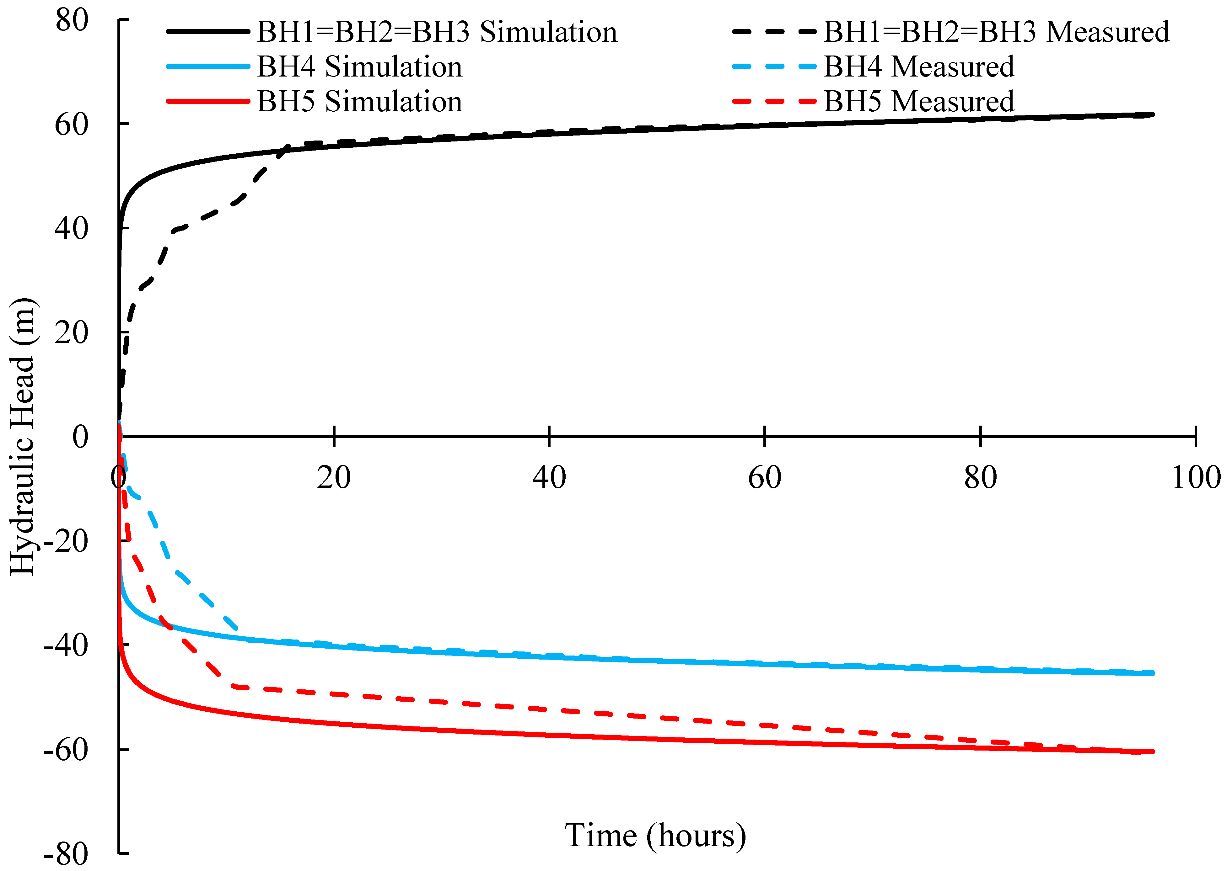
2.5. Model Validation

At the site, numerous tests have been conducted to assess the pumping capacity of the wells. The results indicate that groundwater injection and abstraction significantly disturb the water table. A transient 3D simulation was conducted over a 96 h period to validate the numerical model using data from field experiments. The simulation aimed to replicate the drawdown caused by injection and abstraction in the field test, with specified rates of 8 L per second for abstraction and 5.3 L per second for injection. The simulation outcomes were then compared to the actual field data, revealing close agreement (see Figure 5).

2.6. Material Properties

Material properties for FEFLOW simulations have a significant impact on thermal plume development [2,29]. Therefore, it is important to consider all parameters used in the simulations to be able to achieve realistic results. In this study, the porosity and thermal conductivity of the solid were taken from the literature [30,31]. The other properties, such as the volumetric heat capacity of the fluid and solid, thermal conductivity of the fluid, and longitudinal and transverse dispersibility, were default values given in FEFLOW. The horizontal and vertical hydraulic conductivities of each layer were obtained from the validation analysis. Some of the material properties used for the simulations are presented in

Table 1. Material properties used in the simulation.

Geological Formation	Ground Depth (m)	Horizontal Hydraulic Conductivity (m/s)	Vertical Hydraulic Conductivity (m/s)	Thermal Conductivity of Solid (j/m/s/k)	Thermal Conductivity of Fluid (j/m/s/k)	Porosity	Volumetric Heat Capacity of Solid (MJ/m3/K)	Volumetric Heat Capacity of Fluid (MJ/m3/K)
Topsoil/Made Ground, Sand and Gravels	0–6	5 × 10−4	5 × 10−5	1.5	0.6	0.34	2.52	4.2
Thames Group	6–50	5.8 × 10−11	5.8 × 10−12
Lambeth Group and Thanet Sands	50–72	2 × 10−8	2 × 10−9
White Chalk Subgroup *	72–154	1 × 10−6–3.9 × 10−6	1 × 10−7–3.9 × 10−7	1.87
White Chalk Subgroup **	154–185			1.96
White Chalk Subgroup ***	185–275	8 × 10−8–8 × 10−9	8 × 10−9–8 × 10−10	1.8
Gault Clay	275–300	8.3 × 10−12	8.3 × 10−13	1.5

* Upper parts of the chalk, ** middle parts of the chalk, *** lower parts of the chalk.

.

2.7. Scenarios

In this study, four different scenarios were considered: continuous heating, heating and recovery, heating and cooling, and ATES. The abbreviations and heating/cooling periods per year for each scenario are shown in

Table 2. Abbreviations and heating/cooling periods per year for each scenario.

Numerical Simulations (Scenarios)	Abbreviation	Heating Period (Months per Year)	Cooling Period (Months per Year)
Continuous heating	CH	12	0
Heating and recovery	HR	10
Heating and cooling	HC		2
Aquifer thermal energy storage	ATES

.

Figure 6 shows the total heating demand, designed heat pump output and designed thermal energy obtained from groundwater with COP of 3.91. As expected, the heating demand is higher in winter compared to the heating demand in summer. Therefore, different injection and abstraction rates were applied in the simulations.

In continuous heating (CH), the system provides continuous space heating year-round. It requires continuous injection of cold water into the aquifer. This operation is the one used in the field study considered. To accommodate varying monthly thermal loads, different injection and abstraction rates were applied throughout the year, as shown in Figure 7a. This same annual configuration was simulated over a 100-year period. During this operation, the injection temperature remained constant at 5 °C.

In heating and recovery (HR), the simulation was designed to provide ten months of space heating and two months of recovery each year. The purpose of this configuration is to allow the soil to recover from the heating operation. Since cold water is injected into the soil, the soil temperature decreases. However, by implementing a 2-month recovery period, the soil temperature can be restored, resulting in an increase in temperature around the injection wells. The recovery period is during July and August when the designed heating load is lowest. The annual configuration was maintained for a 100-year simulation, and the injection and abstraction flow rates throughout the year are presented in Figure 7b. The injection temperature during the heating operation was set at 5 °C.

In heating and cooling operation (HC), it was aimed to supply space heating for ten months and space cooling for two months, specifically July and August, when heating demand is lowest and cooling demand is highest. The annual heating and cooling plan was simulated for 100 years. Figure 7c illustrates the injection and abstraction rates applied during a year. With this operation, the system can meet the cooling demand of the buildings. Moreover, as warmer water is injected into the wells during the space cooling, the soil temperature around the injection wells increases. The injection temperature during the heating period is 5 °C, whilst is 35 °C during the cooling period.

The aquifer thermal energy storage operation (ATES) also includes ten months of space heating and two months of space cooling. As in the HC scenario, the cooling demand was in July and August. In the ATES system, the injection and abstraction wells are swapped between the heating and cooling operations to store energy for the subsequent cycle (heating or cooling). Thus, wells used for injection during cooling serve as abstraction wells during heating, and vice versa.

Figure 7d shows the annual injection and abstraction flow rates for the ATES system. There are three injection and two abstraction wells in the field-scale case study. However, in ATES operation, during the heating period (July and August), there are two injection and three abstraction wells, as the wells are swapped. While the abstraction rate per well remains consistent with other scenarios, the total abstraction rate is 27 L/s during heating because of the three abstraction wells. The injection rate per borehole must be 13.5 L/s to inject the abstracted groundwater back into the aquifer, as two wells serve as injection wells during the heating period. Injection and abstraction rates during the cooling period remain the same as in other scenarios. The ATES simulation spans 100 years, with an injection temperature of 5 °C during heating and 35 °C during cooling.

2.8. Optimization

Optimizing a GWHP system, especially at a district level, involves carefully evaluating several critical factors. These include the hydrogeological assessment of the site, the analysis of groundwater movement, the distance between injection and abstraction wells, the rates at which water is injected and extracted, the temperature of the injected and extracted water, regulations and permits, plans for system monitoring and maintenance, and the choice of the operational mode of the system. All of these parameters need to be taken into account during the initial design phase to determine the best possible system setup.

The main focus of this particular study is on optimizing the operational mode of the system, which depends on the heating and cooling needs of the buildings. The system can be configured to provide only heating, only cooling, or a combination of both, depending on the requirements. To determine the most efficient operational mode, we employed a simulation tool called FEFLOW. Various scenarios were considered, as previously mentioned, taking into account factors like the extracted water temperature and whether thermal feedback occurs, as these factors significantly affect the performance of the system.

3. Results and Discussion

3.1. Impact of Thermal Feedback on Abstraction Temperature

The results presented in this section were obtained from the observation points located at a depth of 135 m bgl, as the highest thermal changes were recorded at this depth. In the first three operations, CH, HR and HC, BH4 and BH5 were used for abstraction. It can be seen in Figure 8 that the temperature change in BH5 is negligible. However, the thermal plume reaches BH4 in these three scenarios. The observed temperature in BH4 started decreasing almost 60, 70, and 65 years after the commencement of the simulation in the CH, HR and HC operations, respectively. That was calculated depending on the time it takes to observe a 0.2 °C decrease compared to the temperature of the stabilized period. At the end of 100 years’ simulation, the observed temperature at BH4 is 11.3 °C, 11.6 °C and 12 °C, with a reduction of 10%, 8% and 5%, considering the initial temperature in the CH, HR and HC operations, respectively.

The trend in the temperature change in the ATES operation is different from the other operations (see Figure 9). In the ATES operation, BH1, BH2 and BH3 were used as an abstraction well, and BH4 and BH5 were used as an injection well during the cooling period. Therefore, the operation causes a significant change in the observed temperature in each well during 100 years of operation. To better understand the temperature change in the boreholes, the temperature changes in the first and last year are shown in Figure 9b,c. In the first year, the observed temperatures at BH1, BH2 and BH3 equal the injection temperature, which is 5 °C, during the heating period. When the cooling period starts, around the 180th day, the recovery in these boreholes was observed until the next heating period starts. However, in the last year of the simulation, the observed temperature at these boreholes was stable at 5 °C due to the high volume of injection during the heating period.

In the first year, the temperature observed at BH4 and BH5 remained constant at 12 °C until the cooling period, during which it rapidly increased to 35 °C at BH4 and BH5. This increase is a result of the warmer water injection. At the end of the first year, the observed temperature at BH4 and BH5 decreased to 14.3 °C. In the last year, the observed temperature at BH4 and BH5 is 28% higher than the first year at the beginning of the first heating operation, with an observed value of around 15.3 °C. That is due to the stored warmer water from the previous (cooling) operation. Then, it decreased gradually from 15.3 °C to 13.5 °C. A sudden increase can be observed at the beginning of the cooling period due to warmer water injection. The observed temperature at BH4 and BH5 increased to 35 °C. When the second heating period started, the temperature decreased from around 35 °C to 14.8 °C in BH4 and to 15.4 °C in BH5. The 4% difference in the observed temperature is due to the difference between borehole depths (200 m in BH4 and 135 m in BH5).

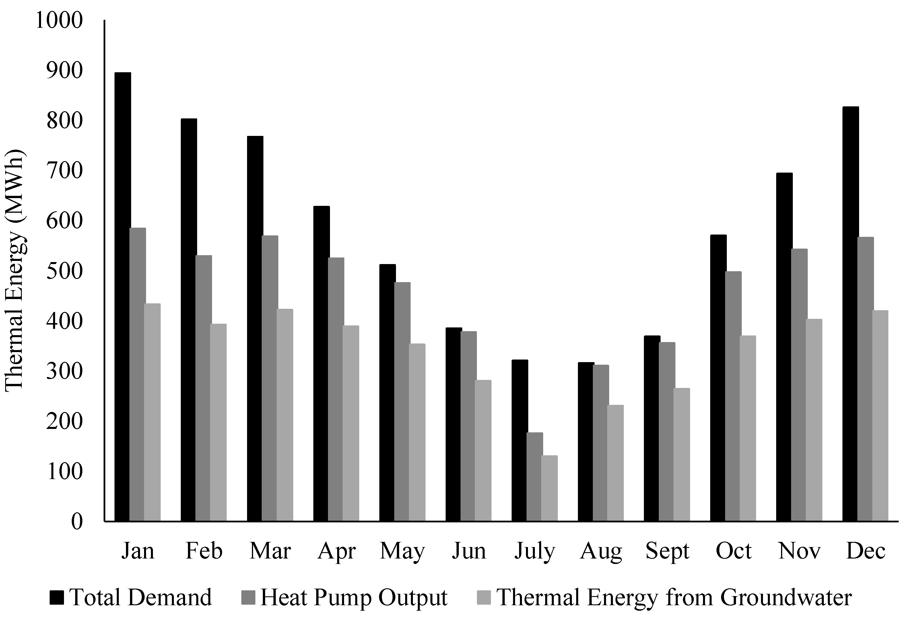
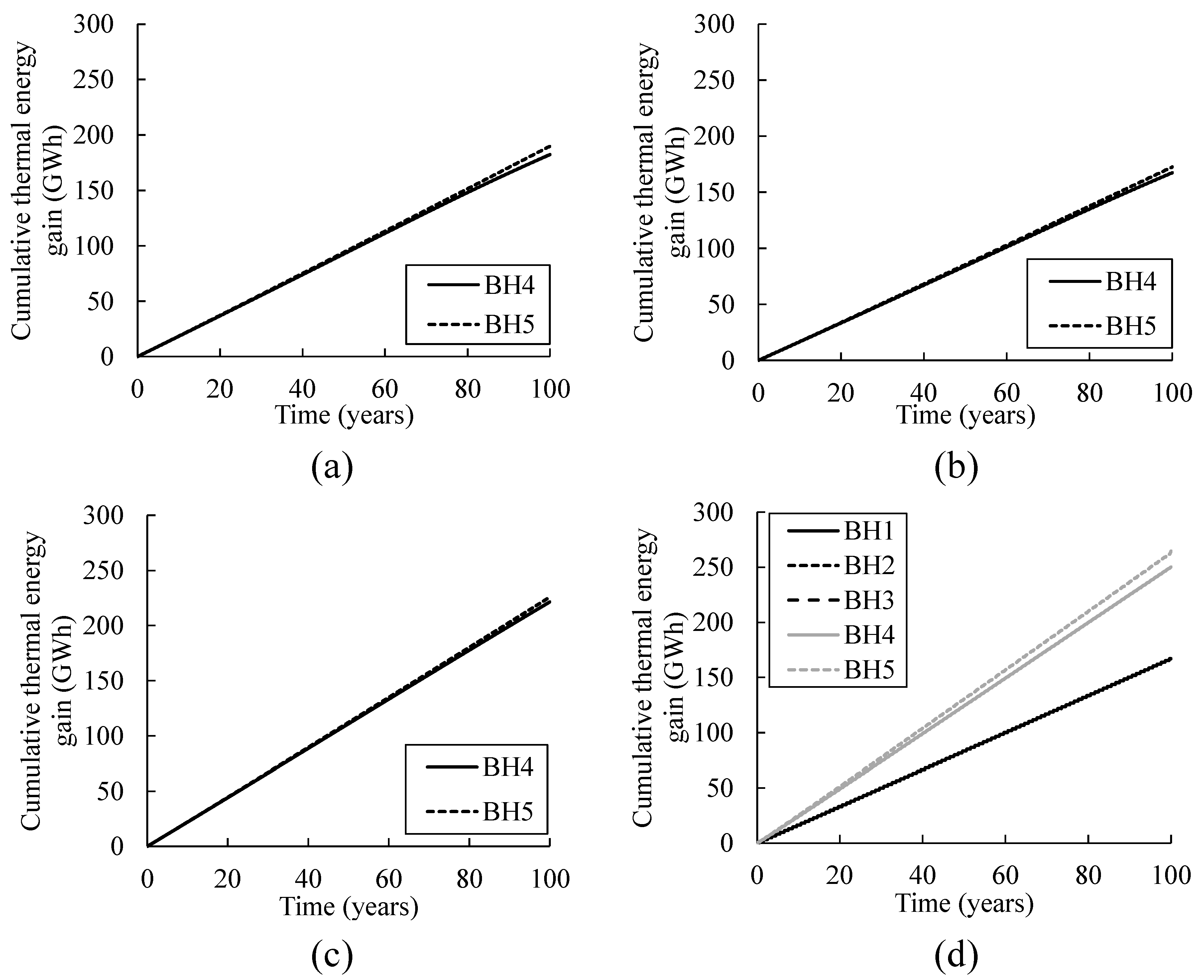
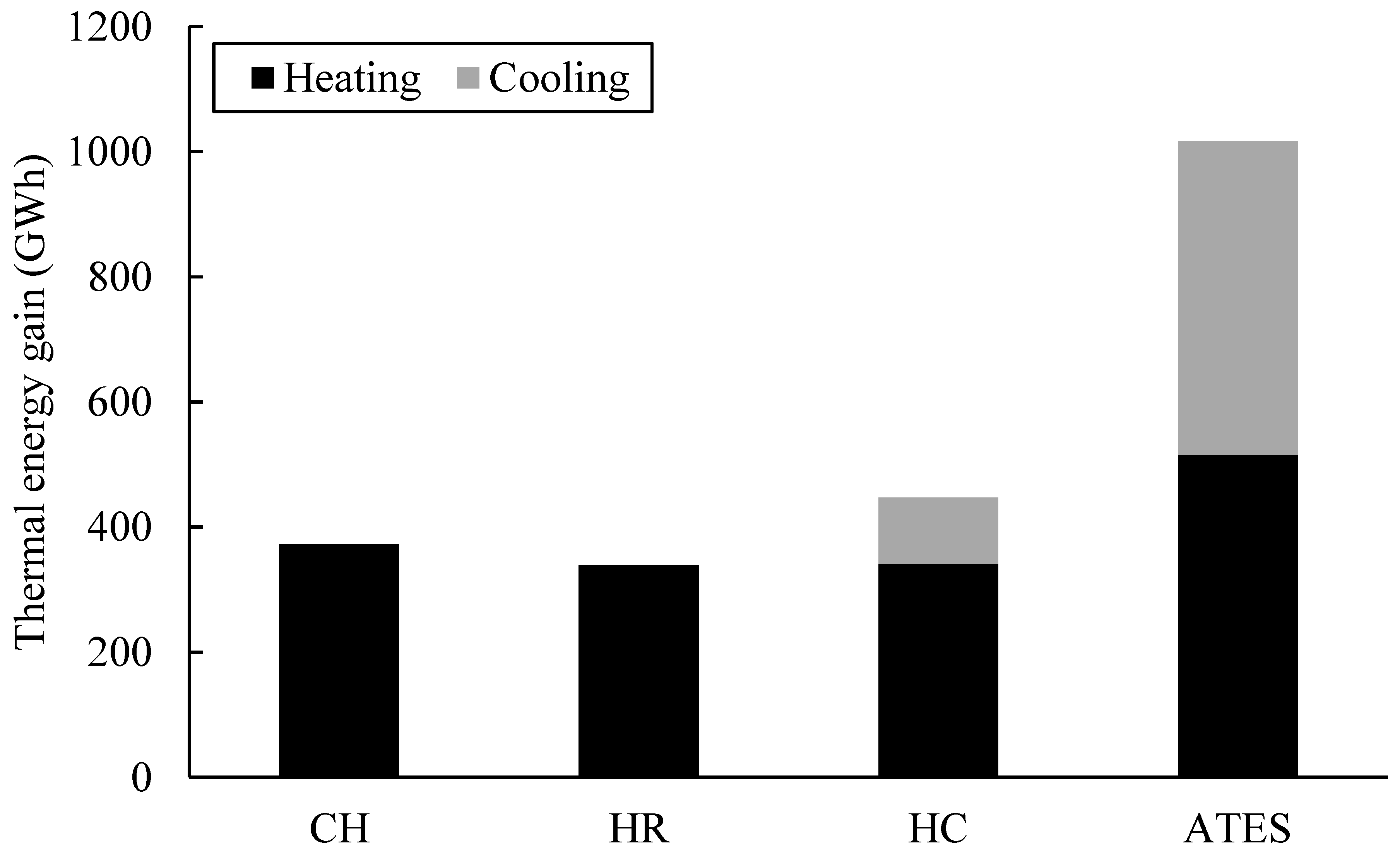
3.2. Thermal Energy Calculations

The thermal energy gain from the groundwater can be calculated using the equation provided below. It accounts for the time-dependent abstraction temperature variations in different scenarios, attributed to thermal feedback in CH, HR, and HC, as well as water storage effects in the ATES test. The thermal energy calculations were performed using temperature data recorded at the end of each hour:

$$\dot{Q}=\dot{m}{C}_{ave}\Delta T$$

(4)

where $\dot{Q}$ is the thermal energy [kW], $\dot{m}$ is the mass [kg/s], C_ave is the average specific heat calculated at the average temperature [kJ/kgK], and ΔT is the change in temperature [K] [32].

The 100-year cumulative thermal energy gain from each borehole in each scenario is shown in Figure 10. It can be seen that the thermal energy gain from BH4 is slightly lower than that from BH5, since thermal feedback occurs in BH4. Although the thermal impact on the abstraction temperature is higher in the CH than in the HR operation, the thermal energy gained from BH4 is 8% lower in the HR compared to the CH operation due to no energy production in the two-month recovery period applied. However, the thermal energy gain from BH4 is 18% higher in HC than in the CH operation due to the coupled impact of the cooling load applied and the lower temperature change in the abstraction temperature. The thermal energy gain in ATES operation is considerably higher than the other operations because the abstraction temperature increases due to the stored warmer water in the previous period (cooling period). Additionally, the injection and abstraction rate during the cooling period in ATES is 1.5 times higher than in HC operation.

The total thermal energy gain from the system in different scenarios is shown in Figure 11. The total thermal energy gain is 372 and 340 GWh in CH and HR operations, respectively. The 17% difference is due to the two-month recovery period in the HR operation. The thermal energy gain during the HC operation in the heating period is around 341 GWh, which is only 0.4% higher than the HR operation because of including two months of cooling, which decreases the effect of thermal feedback on the system. However, the thermal energy gain in the HC operation is 9% lower than in the CH operation due to two months’ less heating operation. The total thermal energy gain during the heating period in ATES operation is around 515 GWh, which is almost 34% higher than the HR and HC operation and 27% higher than the CH operation. This can be attributed to using the stored warmer water during the cooling period.

The total thermal energy gain during the cooling period at the end of 100 years of operation is 106 and 501 GWh in the HC and ATES operations, respectively. The approximate fivefold difference can be attributed to two reasons. The first one is that the abstraction flow rate in the ATES operation is 50% higher than in the HC operation. The second is that the ATES operation uses the stored cooler water injected into the well during the previous period (heating period).

It can be seen that the ATES operation increases the system efficiency and sustainability thanks to the stored energy in each period (heating or cooling). The space heating needs additional energy input from the heat pump. However, space cooling might not necessarily require additional energy input, meaning that extracted groundwater can be directly used for space cooling thanks to the low source temperature at the site. Although in the HC operation, the thermal energy gain is lower during the heating period compared to the CH operation, it supplies a significant amount of space cooling.

The utilization of an ATES system can increase the thermal energy gain by 173%. However, using this system is not always possible, as the operation depends on the hydrogeological conditions of the site [11]. In addition, the HC system can increase efficiency by 20% without further consideration, as there is no need to change the working principle of the system.

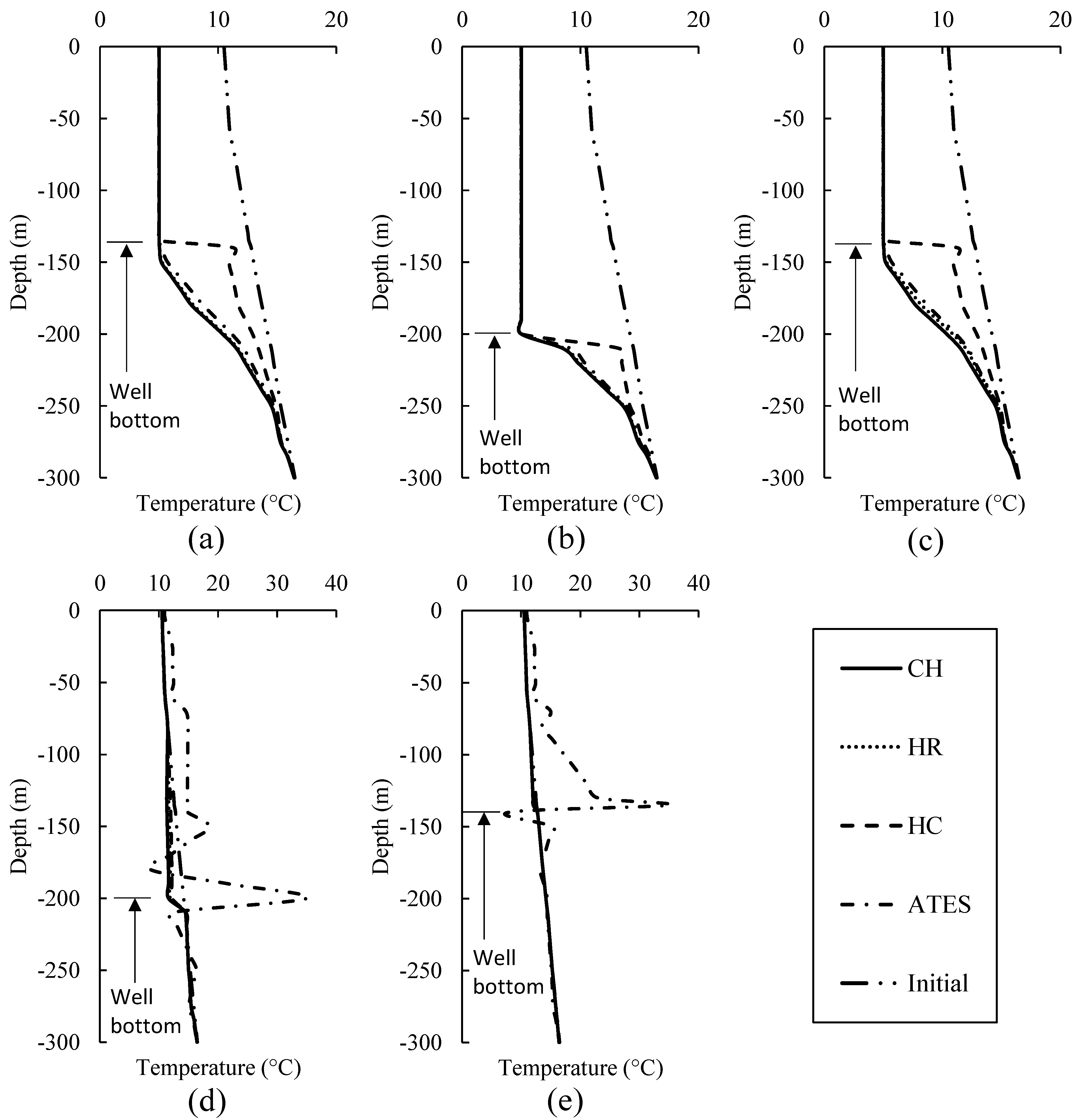
3.3. Vertical Thermal Distribution

The temperature profiles of each well at the end of 100 years of operation are given in Figure 12 and compared with the initial soil temperature. The results were obtained at the perimeter surface of the wells. The soil temperature around the injection wells decreased to a minimum of 5 °C, which is the injection temperature during the heating period. The maximum temperature was observed at BH4 and BH5 as 35 °C, which equals the injection temperature during the cooling period in the ATES operation.

The temperature profiles observed in BH1 and BH3 are almost the same due to having the same soil and borehole depth. In all operations, the observed temperature from top to bottom of the well (from 0 to 135 m bgl) remains consistent at 5 °C, which is also the injection temperature during the heating operation. This result can be attributed to the relatively high volume of injection. Below the bottom of the well, the impact of cold water injection decreased gradually, leading to soil temperature increase from 5 °C to 16.5 °C, which is the initial soil temperature at 300 m bgl. The HC operation created a different pattern in temperature change below the bottom of the well. The temperature increased from 5 °C to 11.3 °C at a depth of between 135 to 140 m bgl, after which a gradual increase was observed for the HC operation until 300 m bgl. The temperature difference between the HC and other scenarios is due to warmer water injection during the cooling period. The warmer water injection increases the temperature of the ground and groundwater. It can also be seen in each scenario that the heat transfer varies with depth. This is due to coupled impact of borehole depth and the hydraulic and thermal conductivity values given to the different layers.

BH2 followed a different pattern, as the borehole depth is 200 m (135 m in BH1 and BH3). As a result, a temperature of 5 °C was observed from the top of the well until the depth of 200 m bgl. Below 200 m, the temperature started increasing in each scenario, but with a higher magnitude in the HC operation due to the warmer water injection during the cooling period.

In the CH, HR and HC operations, the observed temperature from ground level to 80 m bgl is close to the given initial temperature in BH4. Below that level, the temperature remained constant at around 11.6 °C until the depth of 200 m, which is the bottom of BH4. That is due to the thermal feedback impact. The observed temperature between 210 and 300 m bgl is close to that of the initial temperature given. In these three operations, the temperature change in BH5 is negligible, as the thermal plume did not reach BH5. However, the pattern in the temperature change in the ATES operation is different, due to the warmer water injection during the cooling period. The observed temperature in BH4 is slightly higher than the initial temperature at depths of 6 to 140 m bgl, which is around 12 °C at the first 60 m and 14.8 °C below 60 m. The temperature fluctuates between 150 and 250 m bgl with a maximum observed temperature of 35 °C at 200 m bgl, which is the water injection temperature during the cooling period. The changes in the observed temperature can be attributed to variations in the thermal properties at the different depths.

The same situation applies to BH5, where the temperature fluctuates between 80 and 170 m bgl. The maximum temperature was recorded as 35 °C at 135 m bgl in BH5. The difference between the temperature change results in BH4 and BH5 is due to the borehole depth. The warmer water injection during the cooling period creates thermal plume in ATES operation around BH4 and BH5. The warmer water injection is not continuous (July and August). Therefore, the water temperature is expected to recover back to the initial temperature prior to the commencement of the next cooling period, which is after almost 10 months. That would be the case if the operation were performed only for a year. However, as the simulation was performed for 100 years, some parts of the soil could not recover. This is an advantage for an ATES system, as the idea is to store energy for the next operation.

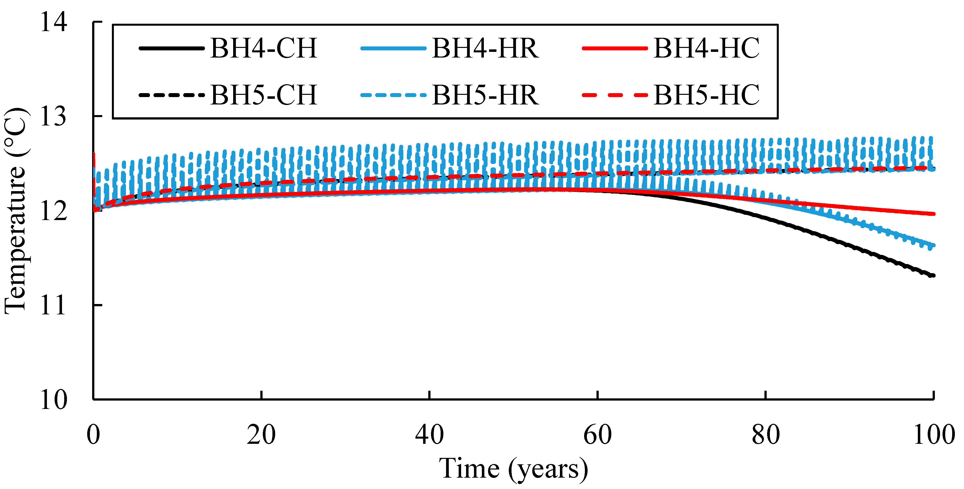
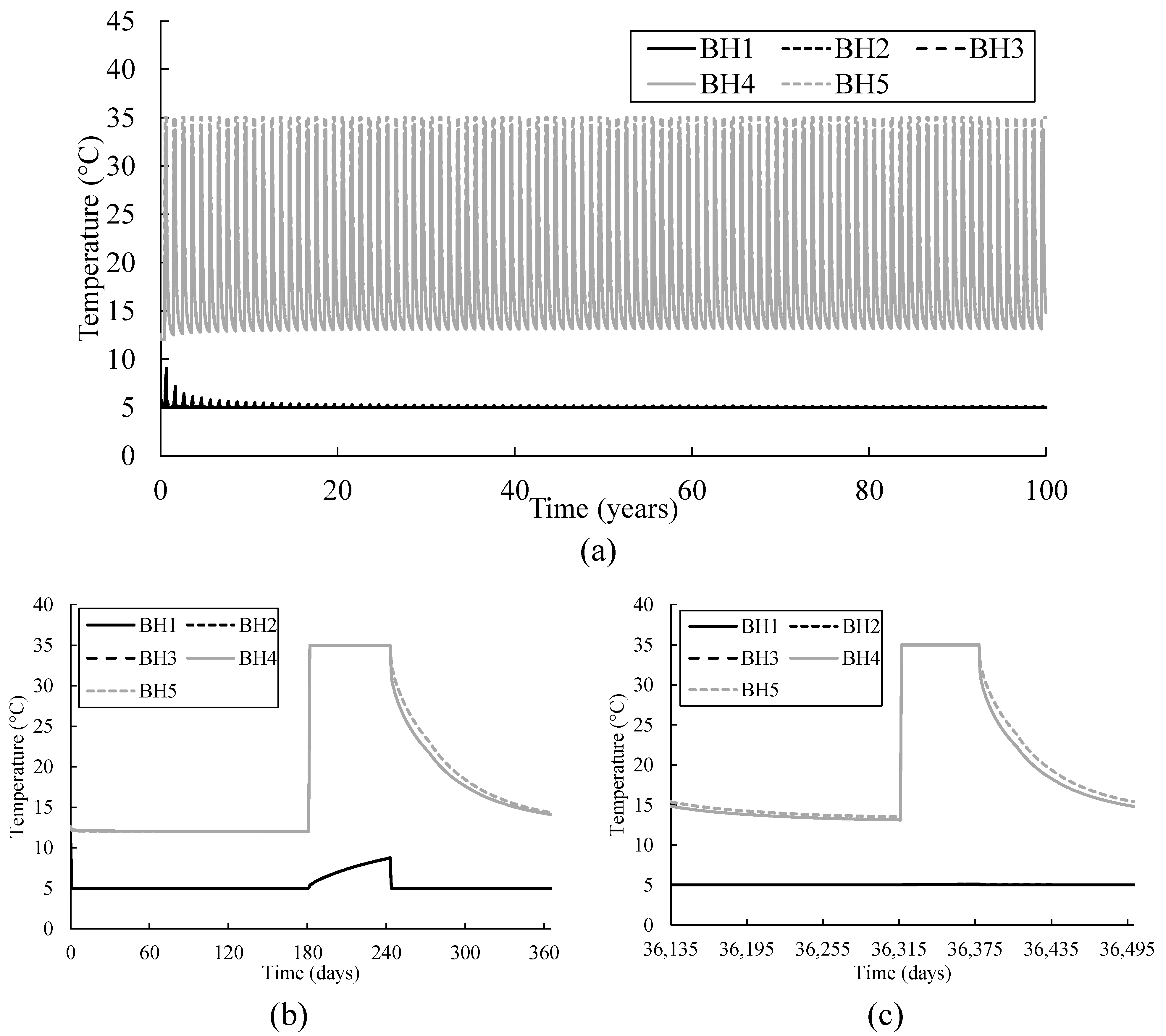
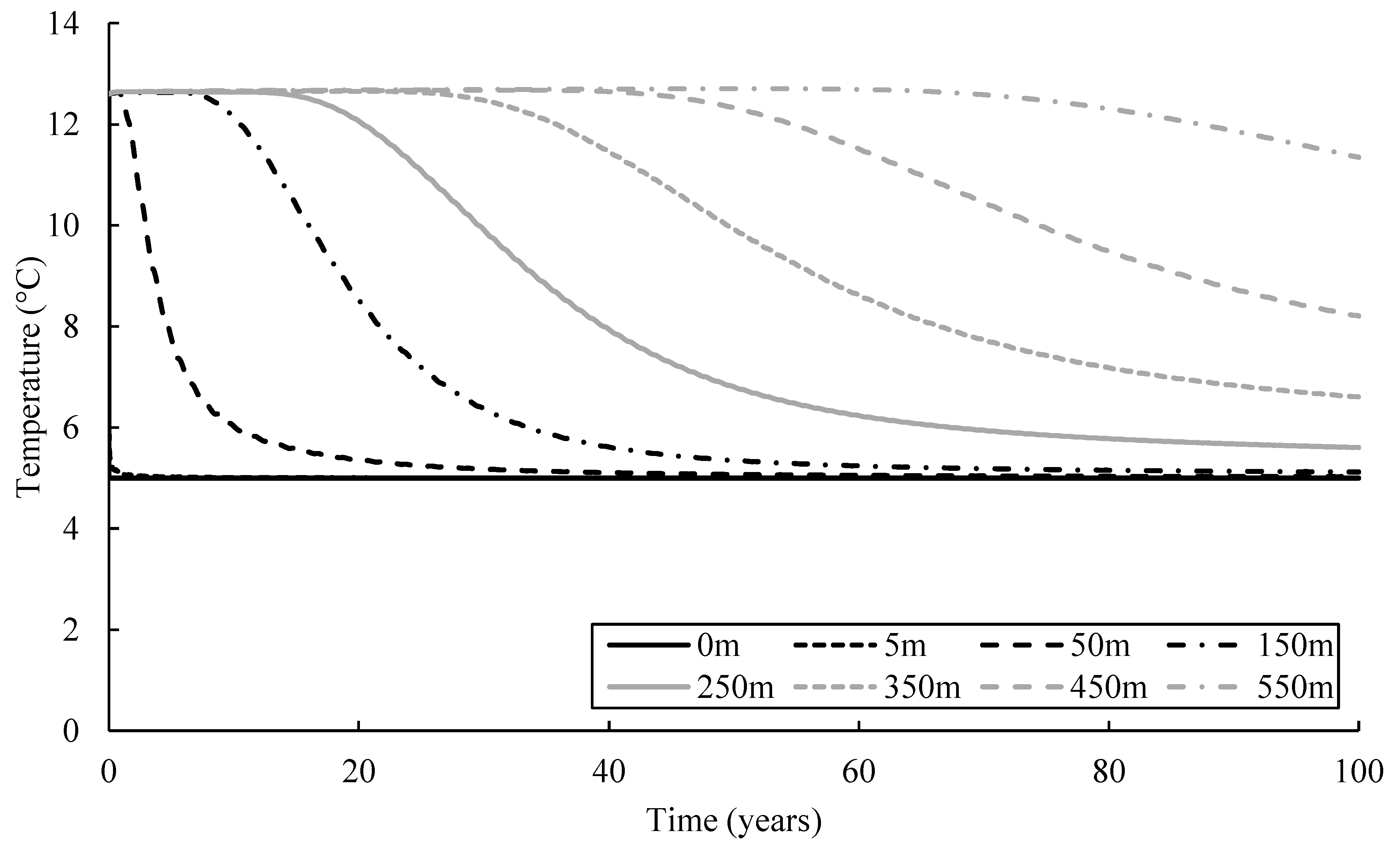
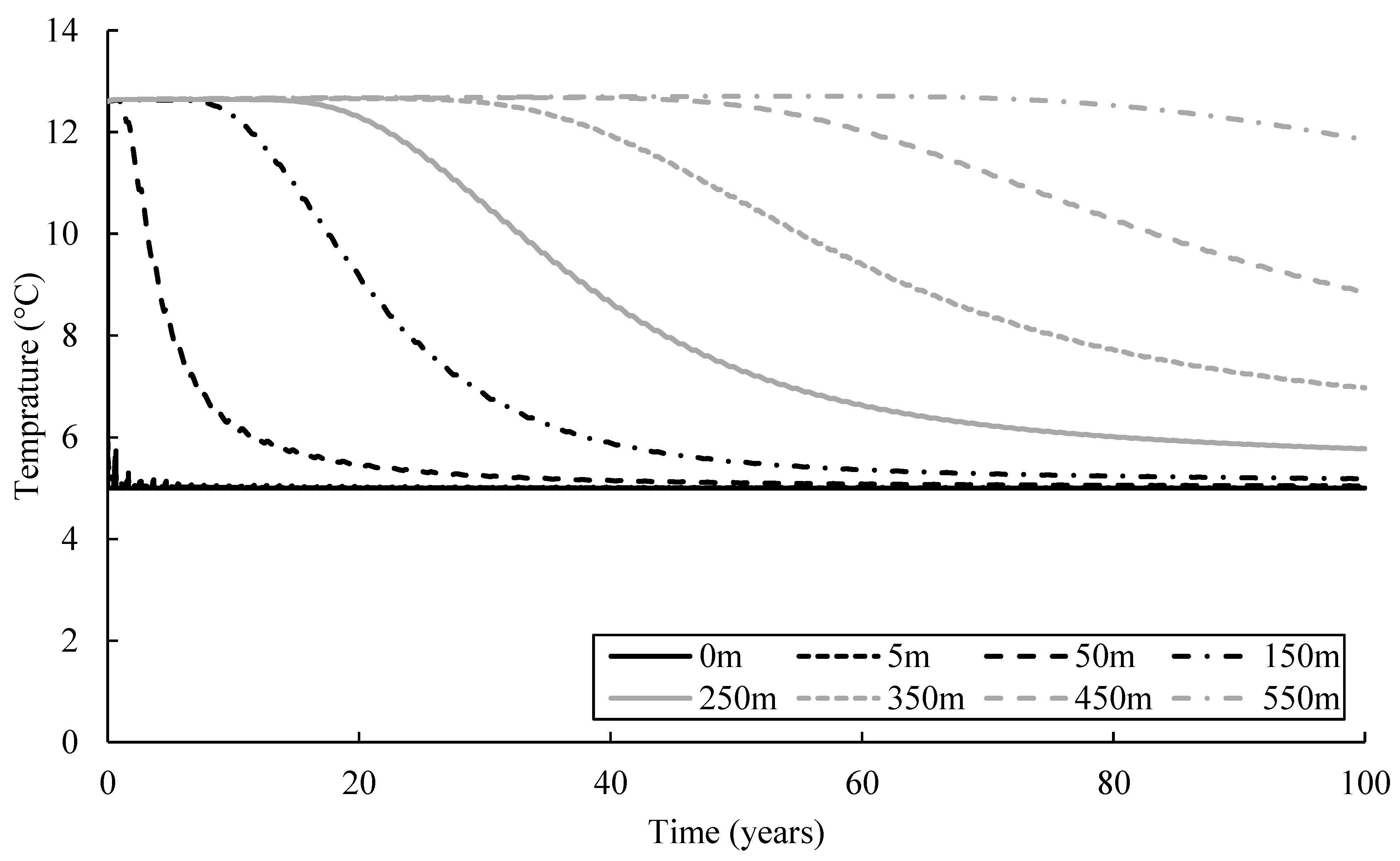
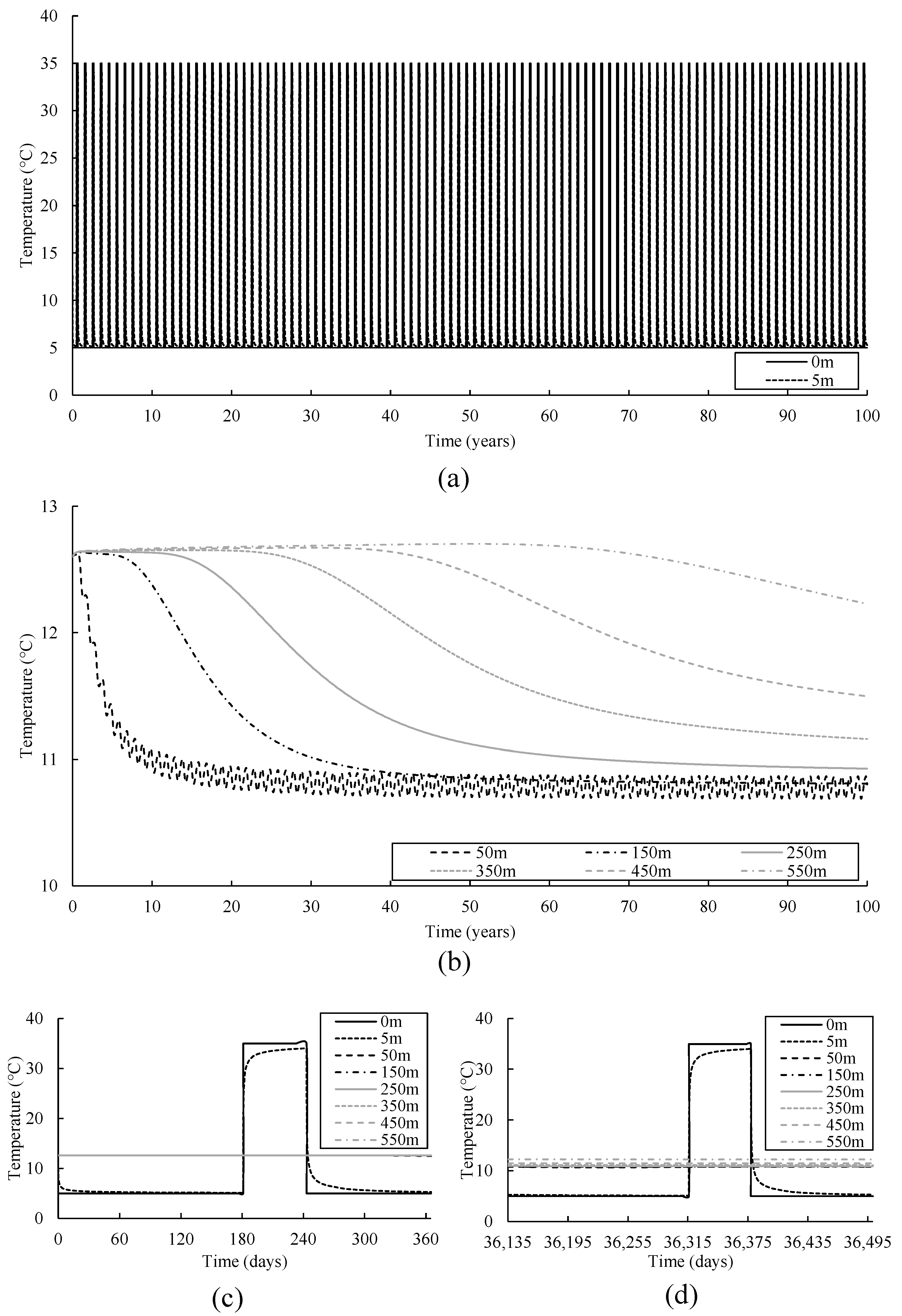
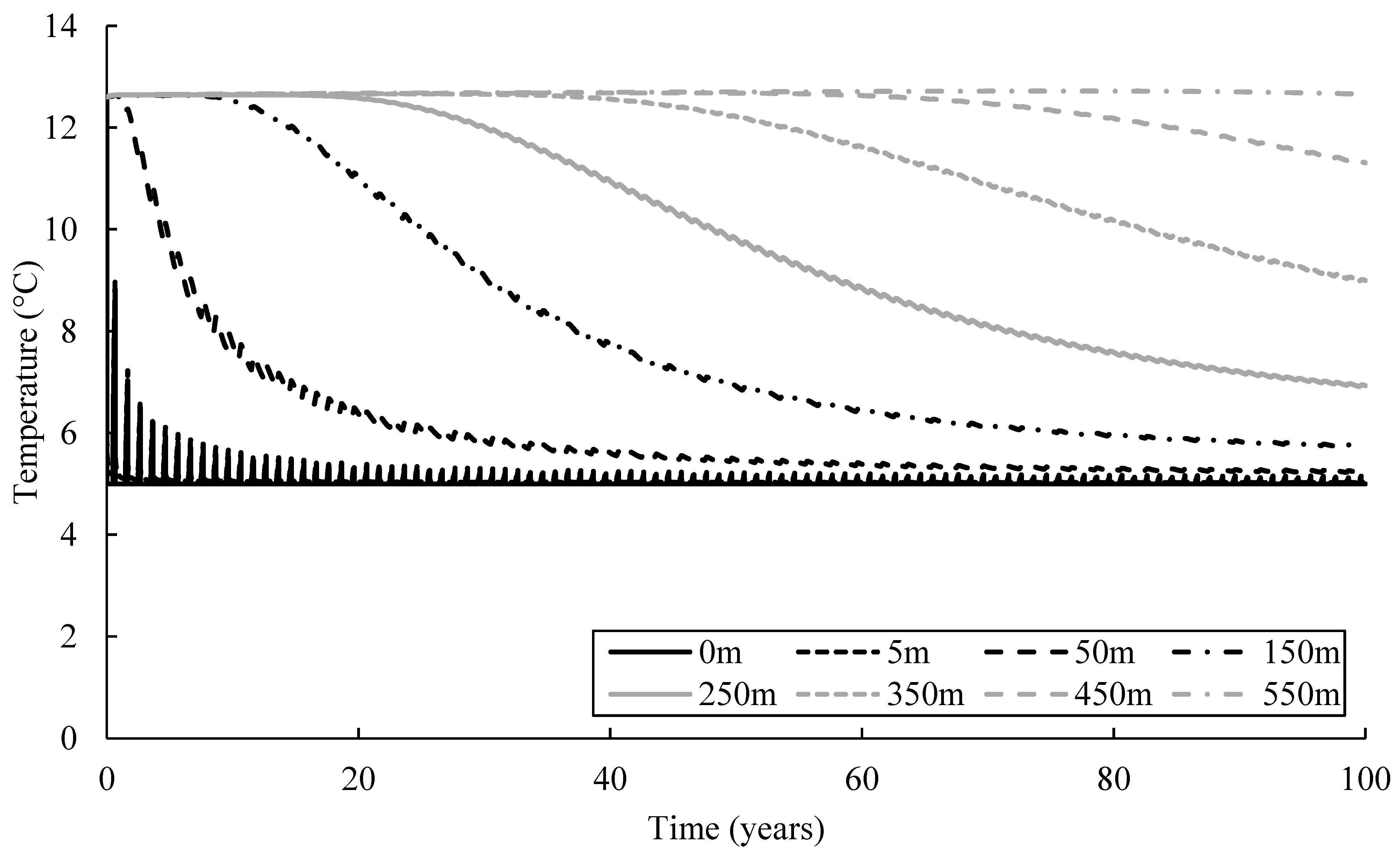
3.4. Temperature Evolution

This section illustrates the results of two-dimensional temperature changes throughout the model domain after 100 years of simulation for each scenario. The results were captured at a depth of 135 m bgl.

It also explains the temperature evolution with time for each scenario. The temperature readings were captured using 10 observation points, starting from the well surface (0 m from the well surface), and ending 550 m away from the well surface. The observation points were chosen depending on the thermal plume dimension. The observed maximum thermal plume dimension is 600 m, considering all scenarios investigated. Therefore, the last observation point was chosen as 550 m, after which thermal change is negligible.

(a) 

Continuous heating test (CH test)

Figure 13 shows a two-dimensional plan view of thermal plume development in the model domain for CH operation at the end of the simulation at 135 m bgl. The minimum temperature observed throughout the model is around 5 °C, which is the injection temperature. A maximum temperature of around 13 °C was observed, which is the undisturbed temperature given at the initial stage. It can be seen that the thermal plume starts from the injection wells and spreads around them. The impact of water injection decreases towards BH4 and BH5. The maximum thermal plume dimension was measured at around 600 m radial distance.

The temperature evolution throughout the simulation time of 100 years at different observation points located downgradient from BH1 is given in Figure 14. The radial temperature distribution observed at 0 and 5 m from the surface of BH1 equals the injection temperature of 5 °C, which is constant during the whole simulation. After almost 45 years, the temperature observed at 50 m away from BH1 decreased to 5 °C. It took nearly 8, 16, 25, 45, and 70 years to observe a decrease at the observation points located 150, 250, 350, 450 and 550 m away from the well surface. These observation points followed a similar pattern where the observed temperature stayed constant until the thermal plume reached the observation point and then decreased until the end of the simulation. The slightest decrease was observed at the farthest observation point, located 550 m away from BH1. At the end of the simulation, the temperature was observed as 11.3 °C, with a decrease of 10% from the initial temperature of 12.6 °C.

(b) 

Heating and recovery test (HR test)

The two-dimensional plan view of radial thermal plume development shown in Figure 15 at the end of the HR simulation is analogous to the CH. However, the thermal plume dimension created by the HR operation is 2% lower than the CH operation, with a maximum measured zone of thermal influence of 590 m radial distance from the wells (BH1–BH3).

The temperature evolution during 100 years of simulation time at different observation points is shown in Figure 16. The thermal change at the given observation points is similar to the CH operation. At the observation points located at 0 and 5 m downgradient of BH1, the temperature suddenly decreased to 5 °C, which remained constant until the end of the simulation. In the first couple of years, the observed temperature fluctuated due to the recovery period. However, after a few years, the recovery impact became negligible, which could be attributed to the relatively large injection flow rate occurring at a temperature of 5 °C. The temperature observed at 50 m suddenly decreased in the first ten years, after which the decrease was gradual. It dropped to almost 5 °C at the end of the simulation. Other observation points also witnessed a delay in temperature reduction away from BH1. The temperature at the farthest observation point, located 550 m away from the well, is 11.85 °C, with a decrease of 6% from the initial temperature of 12.6 °C.

(c) 

Heating and cooling test (HC test)

The two-dimensional plan view of thermal plume development at the end of the simulation for the HC operation is shown in Figure 17. The minimum temperature was observed around the injection wells at 135 m bgl. The temperature decreased significantly around the injection well (at about 10 m radially) due to the cold water injection during the heating period. However, the cooling period impact due to warmer water injection can be observed at a radial distance of 20 m, with an observed temperature of about 12.8 °C. The maximum radial thermal plume zone of influence is at 580 m in this operation.

Figure 18 illustrates the simulation results of temperature readings at different observation points in the HC operation. The temperature observed at 0 and 5 m away from the injection well shaft surface fluctuated during the simulation due to the fluctuation in the water injection temperature, which is 5 °C during the heating period and 35 °C during the cooling period. The observation points located at 50 and 150 m radially from the well surface witnessed a decrease, with an observed temperature of 10.8 °C at the end of the simulation. For the observation points located 250, 350 and 450 m away from BH1, the observed temperature is 10.9 °C, 11.2 °C and 11.5 °C, respectively, after 100 years of operation. The temperature observed at a radial distance of 550 m from the well (farthest observation point) is 12.2 °C, with a decrease of 3% considering the initial temperature of 12.6 °C.

(d) 

ATES test

Figure 19 illustrates the two-dimensional plan view of thermal plume development at the end of the simulation for the ATES operation. The minimum temperature was recorded around the injection wells due to the cold water injection during the heating period. The maximum temperature value of 35 °C given in the color bar is the injection temperature during the cooling period, and it was observed around BH4 and BH5. However, it cannot be seen clearly in the figure, as the radius of the thermal plume around BH4 and BH5 is relatively small. The farthest point affected by the thermal plume is 530 m downgradient of BH1.

As shown in Figure 20, the temperature observed at 0 and 5 m away from BH1 decreased to 5 °C. BH1 was used as an abstraction well, so the temperature fluctuated during the cooling period. The fluctuation can be attributed to the recovery. The magnitude of the temperature fluctuation between the heating and cooling period decreases over time due to the longer duration of the heating period. At the end of the simulation, the observation points located 50 and 150 m radially from the well witnessed a significant decrease, with an observed temperature value of 5.2 °C and 5.7 °C, respectively. The thermal plume reached the observation point 450 m away from the well after almost 60 years, with an observed temperature of 11.3 °C at the end of the simulation. The farthest observation point (550 m) witnessed no temperature change, as the maximum zone of thermal influence is 530 m.

(e) 

Comparison

The main difference between different operations is the dimension of the thermal plume created by the injection. The thermal plume dimension in the HR operation is 2% lower than in the CH operation due to the given recovery period of 2 months (July and August) per year. Adding a cooling period of 2 months annually helps reduce the thermal plume dimension by 3% in the HC operation. Although the ATES operation has the same heating period as the HC operation, the thermal plume dimension is 9% lower in ATES than in the HC operation. Two reasons can explain this result. Firstly, the system operates more efficiently by utilizing thermally stored water. Secondly, the abstraction rate during the cooling period is 1.5 times higher in ATES than in HC.

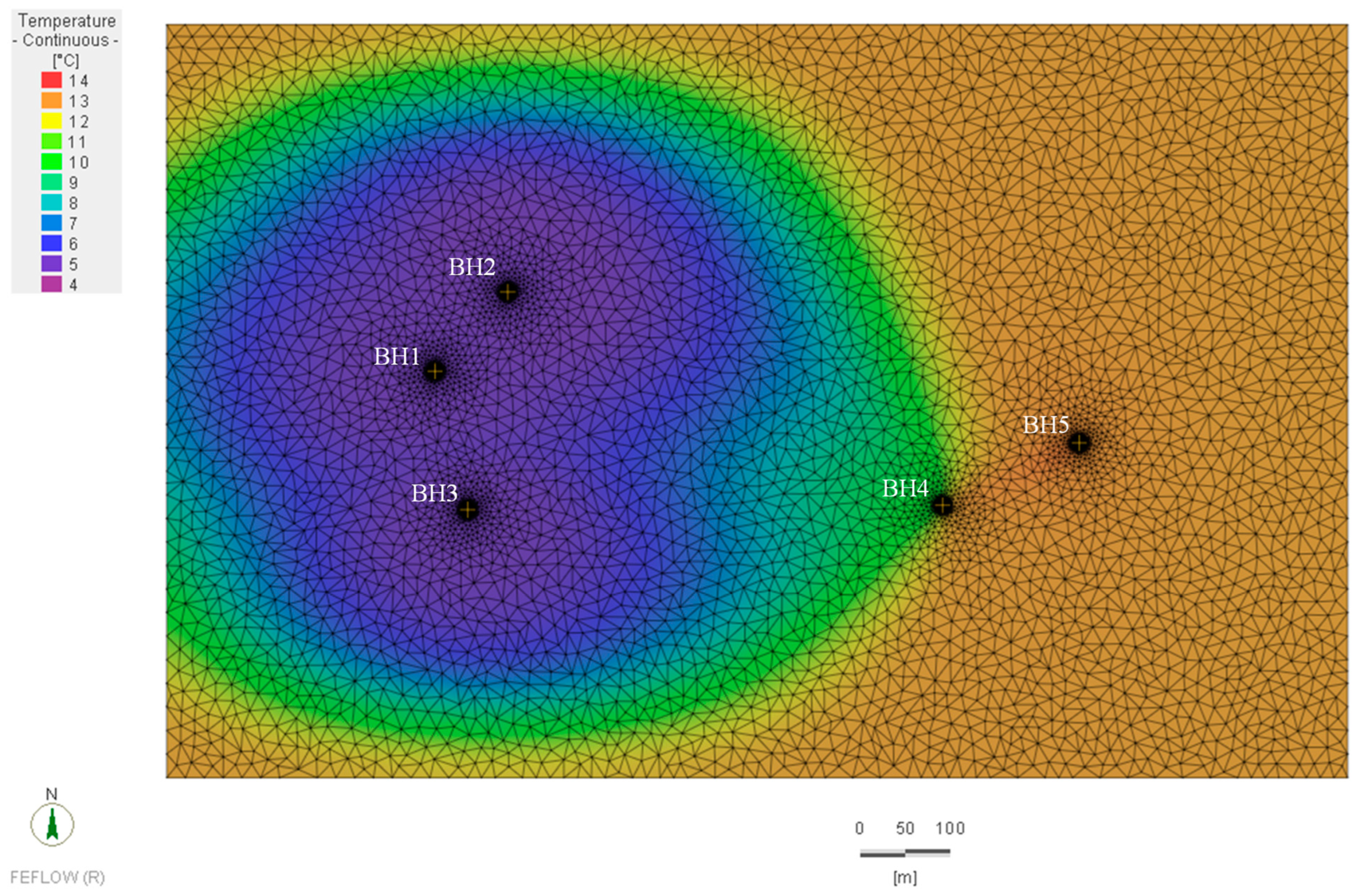
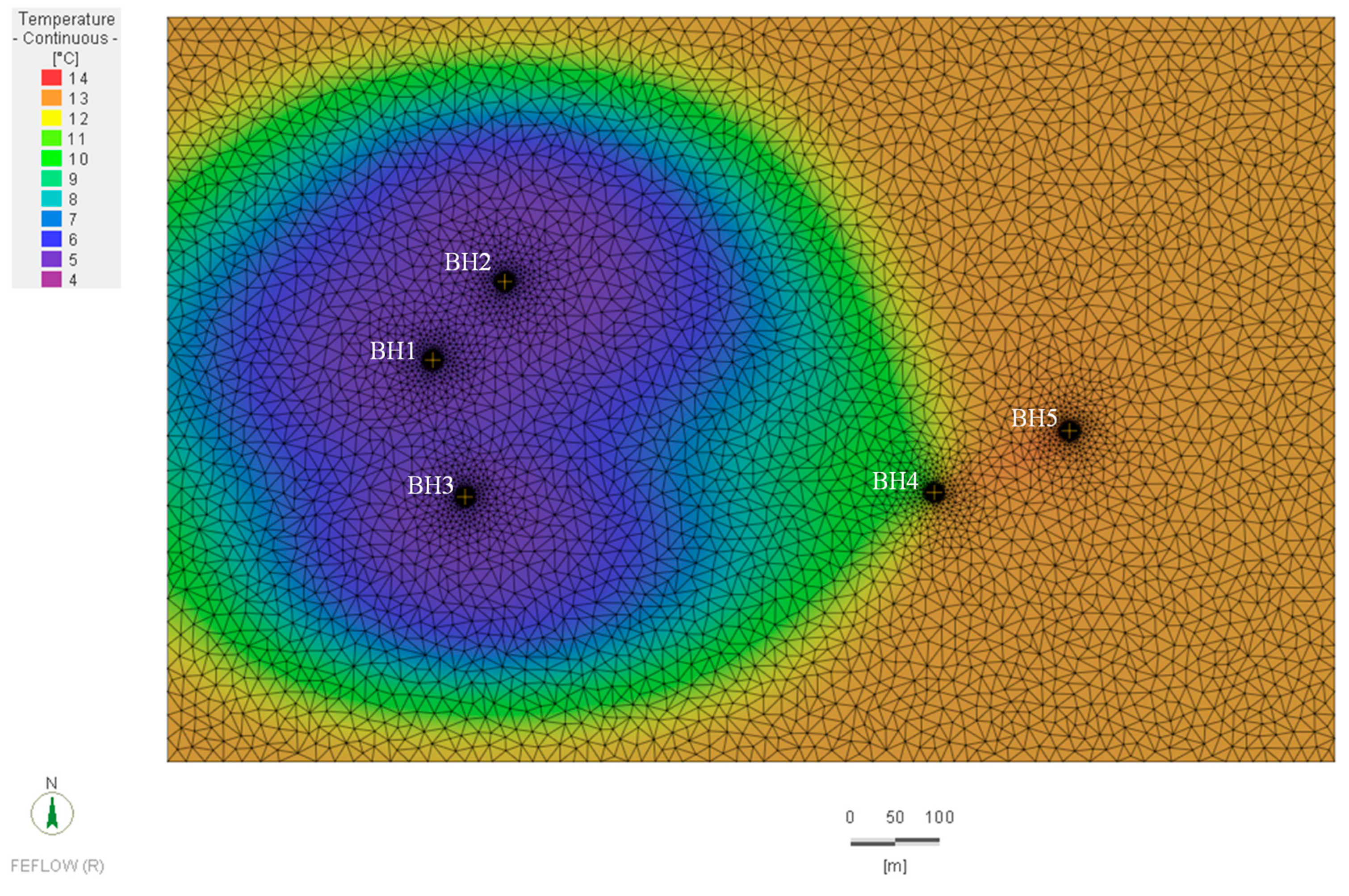
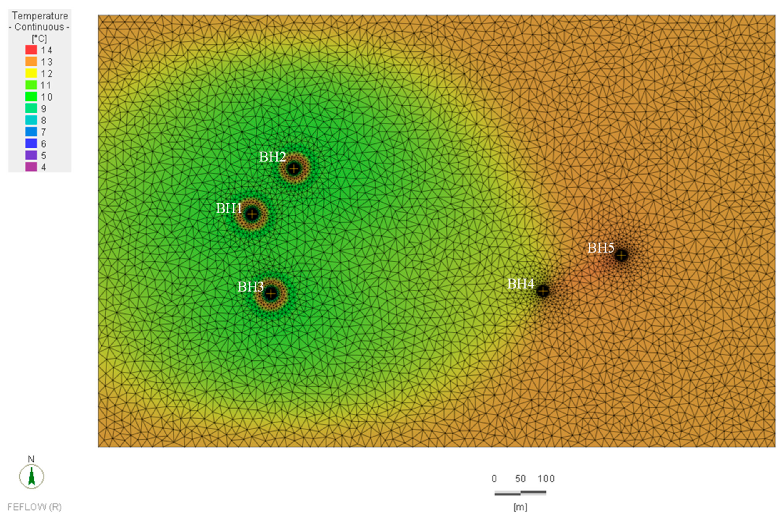
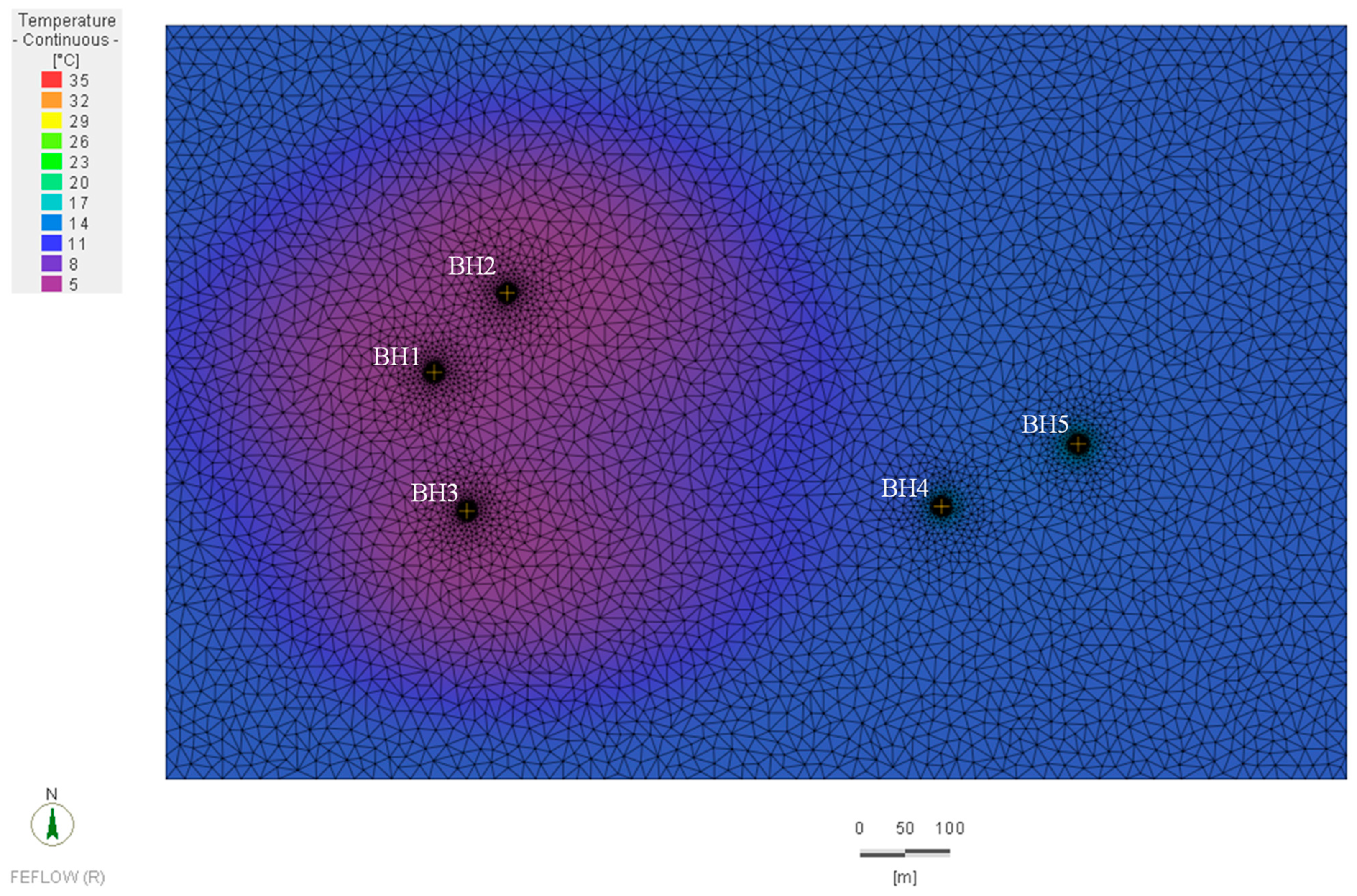
3.5. Thermal Plume Development and Groundwater Flow Impact

Figure 21 shows the temperature distribution at BH1 with a distance from −300 m to 550 m. On the left side of the axis, the values represent the distance from BH1 to the model boundary. On the right side, the values indicate the distance from BH1 to the right side of the model, which is the direction of groundwater flow. The location of BH1 is 0 m on the x-axis. The simulation results show that the change in the observed temperature in all operations decreases with the distance from the injection well, with the maximum change around the injection well and minimum change at the furthest observation point in the groundwater flow direction.

The CH and HR operations follow a similar trend, with a maximum difference of 8% at the observation point located 450 m away from BH1 in the groundwater flow direction. This difference is due to the applied recovery period in the HR operation. The injection temperature of 5 °C can be observed at a 100 m radial distance from the well. After that, the effect of cooler water injection in the well decreases. The observed temperature at the furthest point from BH1 (550 m) is 11.3 °C and 11.8 °C with a temperature decrease of 12% and 7% compared to the initial temperature in CH and HR operations, respectively.

The ATES operation witnessed a similar trend, where the change in the observed temperature decreased with distance from the well. Around the well, the observed temperature is around 5 °C, which increased towards the boundary and groundwater flow direction. The temperature was observed as 10.9 °C at the model boundary (300 m away from BH1 in the boundary direction). The temperature observed at the furthest observation point from the well (550 m) is 12.65 °C, which is slightly higher than the initial temperature. This result can be attributed to the fact that the warmer water injection during the heating period occurring in BH4 and BH5 increases the temperature of the surroundings of the boreholes, as BH4 and BH5 are close to the observation point located 550 m away from the injection well, with a radial distance of 160 m from BH4 and 190 m from BH5.

Compared to other operations, the temperature observed in the HC operation is closer to the initial temperature. The observed temperature is 5 °C at the well surface (i.e., 0 m from the well surface), significantly increasing away from BH1. The observed temperature increased suddenly from 5 °C to 12.2 °C at the observation point located 20 m away from BH1. That is due to the impact of the previous cooling period in which warmer water (at 35 °C) was injected into the borehole. After the end of the cooling period, the injection of cooler water (at 5 °C) decreased the soil temperature close to the borehole. The temperature decreased from 12.2 °C to 10.5 °C between 20 and 40 m away from BH1 in the groundwater flow direction, after which the observed temperature slowly increased from 40 to 550 m, where the temperature was observed as 12.2 °C.

The groundwater flow has an impact on thermal plume development. The results show that the groundwater flow increases the effect of water injection. For instance, the observed temperature at 250 m from the injection well is 5.6 °C in the downstream direction and 6.4 °C in the upstream direction in the CH operation. This trend is the same in each scenario, meaning that the temperature observed at the same observation points equidistant from BH1 is consistently lower in the downstream direction than in the upstream direction. The percentage of the temperature difference depends on the distance from the well and the operation type.

4. Conclusions

This study presented a long-term numerical investigation of the Northern Gateway Heat Network considering four different scenarios: continuous heating, heating and recovery, heating and cooling, and ATES. It also discussed the thermal impact and thermal plume development in different scenarios and how the thermal plume affected the system efficiency. The key findings are as follows.

• Thermal feedback occurs in the CH, HR, and HC operations. The thermal plume reached BH4 in each operation. However, BH5 was not affected by the thermal plume, since it is located 160 m away from BH4.
• It takes around 60, 70 and 65 years to observe a temperature drop of 0.2 °C in the CH, HR, and HC operations, respectively. After 100 years of simulation, the observed temperature in BH4 decreased by 10%, 8%, and 5% in the CH, HR, and HC operations, respectively.
• In the CH, HR, HC and ATES operations, the total thermal energy gained from the groundwater during the heating period is 372, 340, 341, and 515 GWh over 100 years, respectively. During the cooling period, it is approximately 106 and 501 GWh in the HC and ATES operations, respectively.
• The HR operation decreases the thermal impact observed in the abstraction temperature. However, the thermal energy gain from the groundwater in HR operation is lower than CH due to no energy production in the recovery time of two months per year. The HC operation also decreases the thermal impact on the abstraction temperature compared to the CH. The thermal energy gain during the heating period in the HC operation is relatively higher than in the HR operation, but lower than in the CH operation. The thermal energy gain during the heating period is 38% higher in ATES than in CH due to the use of stored thermal energy during the cooling period.
• The thermal energy gain during the cooling period in the ATES operation is approximately fivefold the HC operation. This result can be attributed to two reasons. First, the ATES operation uses the stored cooler water during the heating period, which increases the thermal energy gain by increasing ΔT. Second, the abstraction rate during the cooling period in the ATES operation is 50% higher than in the HC operation because the ATES operation uses three wells to abstract water from the aquifer, whilst the HC operation uses two wells.
• The utilization of an ATES system can lead to a 173% increase in thermal energy gain compared to the actual system operation. However, its feasibility depends on the hydrogeological conditions of the site. On the other hand, implementing an HC system can enhance efficiency by 20% without the need to change the working principle of the system.
• Groundwater flow has a considerable impact on thermal plume development. It disperses the thermal plume in the groundwater flow direction, resulting in greater thermal changes.

References

1. D’Agostino, D.; Cuniberti, B.; Bertoldi, P. Energy consumption and efficiency technology measures in European non-residential buildings. Energy Build. 2017, 153, 72–86. [Google Scholar] [CrossRef]
2. Russo, S.L.; Taddia, G.; Verda, V. Development of the thermally affected zone (TAZ) around a groundwater heat pump (GWHP) system: A sensitivity analysis. Geothermics 2012, 43, 66–74. [Google Scholar] [CrossRef]
3. Blázquez, C.S.; Verda, V.; Nieto, I.M.; Martín, A.F.; González-Aguilera, D. Analysis and optimization of the design parameters of a district groundwater heat pump system in Turin, Italy. Renew. Energy 2020, 149, 374–383. [Google Scholar] [CrossRef]
4. Singh, R.M.; Sani, A.K.; Amis, T. An overview of ground-source heat pump technology. In Managing Global Warming: An Interface of Technology and Human Issues; Academic Press: Cambridge, MA, USA, 2019. [Google Scholar]
5. Casasso, A.; Tosco, T.; Bianco, C.; Bucci, A.; Sethi, R. How Can We Make Pump and Treat Systems More Energetically Sustainable? Water 2019, 12, 67. [Google Scholar] [CrossRef]
6. Florides, G.; Kalogirou, S. Ground heat exchangers—A review of systems, models and applications. Renew. Energy 2007, 32, 2461–2478. [Google Scholar] [CrossRef]
7. Galgaro, A.; Cultrera, M. Thermal short circuit on groundwater heat pump. Appl. Therm. Eng. 2013, 57, 107–115. [Google Scholar] [CrossRef]
8. Banks, D. Thermogeological assessment of open-loop well-doublet schemes: A review and synthesis of analytical approaches. Hydrogeol. J. 2009, 17, 1149–1155. [Google Scholar] [CrossRef]
9. Bloemendal, M.; Olsthoorn, T.; Boons, F. How to achieve optimal and sustainable use of the subsurface for Aquifer Thermal Energy Storage. Energy Policy 2014, 66, 104–114. [Google Scholar] [CrossRef]
10. Gao, L.; Zhao, J.; An, Q.; Wang, J.; Liu, X. A review on system performance studies of aquifer thermal energy storage. Energy Procedia 2017, 142, 3537–3545. [Google Scholar] [CrossRef]
11. Fleuchaus, P.; Schüppler, S.; Godschalk, B.; Bakema, G.; Blum, P. Performance analysis of Aquifer Thermal Energy Storage (ATES). Renew. Energy 2019, 146, 1536–1548. [Google Scholar] [CrossRef]
12. Dickinson, J.S.; Buik, N.; Matthews, M.C.; Snijders, A. Aquifer thermal energy storage: Theoretical and operational analysis. 2009, 59, 249–260. Geotechnique 2009, 59, 249–260. [Google Scholar] [CrossRef]
13. Bonte, M.; Van Breukelen, B.M.; Stuyfzand, P.J. Environmental impacts of aquifer thermal energy storage investigated by field and laboratory experiments. J. Water Clim. Chang. 2013, 4, 77–89. [Google Scholar] [CrossRef]
14. Park, D.; Lee, E.; Kaown, D.; Lee, S.-S.; Lee, K.-K. Determination of optimal well locations and pumping/injection rates for groundwater heat pump system. Geothermics 2021, 92, 102050. [Google Scholar] [CrossRef]
15. Halilovic, S.; Böttcher, F.; Kramer, S.C.; Piggott, M.D.; Zosseder, K.; Hamacher, T. Well layout optimization for groundwater heat pump systems using the adjoint approach. Energy Convers. Manag. 2022, 268, 116033. [Google Scholar] [CrossRef]
16. Pophillat, W.; Attard, G.; Bayer, P.; Hecht-Méndez, J.; Blum, P. Analytical solutions for predicting thermal plumes of groundwater heat pump systems. Renew. Energy 2020, 147, 2696–2707. [Google Scholar] [CrossRef]
17. Russo, S.L.; Civita, M.V. Open-loop groundwater heat pumps development for large buildings: A case study. Geothermics 2009, 38, 335–345. [Google Scholar] [CrossRef]
18. Russo, S.L.; Gnavi, L.; Roccia, E.; Taddia, G.; Verda, V. Groundwater Heat Pump (GWHP) system modeling and Thermal Affected Zone (TAZ) prediction reliability: Influence of temporal variations in flow discharge and injection temperature. Geothermics 2014, 51, 103–112. [Google Scholar] [CrossRef]
19. Russo, S.L.; Taddia, G.; Baccino, G.; Verda, V. Different design scenarios related to an open loop groundwater heat pump in a large building: Impact on subsurface and primary energy consumption. Energy Build. 2011, 43, 347–357. [Google Scholar] [CrossRef]
20. Halilovic, S.; Odersky, L.; Hamacher, T. Integration of groundwater heat pumps into energy system optimization models. Energy 2021, 238, 121607. [Google Scholar] [CrossRef]
21. Biglia, A.; Ferrara, M.; Fabrizio, E. On the real performance of groundwater heat pumps: Experimental evidence from a residential district. Appl. Therm. Eng. 2021, 192, 116887. [Google Scholar] [CrossRef]
22. Kranz, S.; Bartels, J. Simulation and Data Based Optimisation of an Operating Seasonal Aquifer Thermal Energy Storage. In Proceedings of the World Geothermal Congress 2010, Bali, Indonesia, 25–29 April 2010. [Google Scholar]
23. Halilovic, S.; Böttcher, F.; Zosseder, K.; Hamacher, T. Optimizing the spatial arrangement of groundwater heat pumps and their well locations. Renew. Energy 2023, 217, 119148. [Google Scholar] [CrossRef]
24. Boon, D.P.; Butcher, A.; Townsend, B.; Woods, M.A. Geological and Hydrogeological Investigations in the Colchester Northern Gateway Boreholes: February 2020 Survey; British Geological Survey: Nottingham, UK, 2020. [Google Scholar]
25. Birks, D.; Coutts, C.A.; Younger, P.L.; Parkin, G. Development of A Groundwater Heating and Cooling Scheme in A Per-Mo-Triassic Sandstone Aquifer in South-West England and Approach to Managing Risks. Geosci. South-West Engl. 2015, 13, 428–436. Available online: http://eprints.gla.ac.uk/116692/ (accessed on 28 July 2022).
26. Boon, D.P.; Farr, G.J.; Abesser, C.; Patton, A.M.; James, D.R.; Schofield, D.I.; Tucker, D.G. Groundwater heat pump feasibility in shallow urban aquifers: Experience from Cardiff, UK. Sci. Total. Environ. 2019, 697, 133847. [Google Scholar] [CrossRef]
27. Diersch, H.-J.G. FEFLOW: Finite Element Modeling of Flow, Mass and Heat Transport in Porous and Fractured Media; Springer: Berlin/Heidelberg, Germany, 2014; pp. 1–996. [Google Scholar] [CrossRef]
28. De-wit, E. Pumping Test Factual Report Project Name: Colchester Northern Gateway Heat Network Stage Gate 4 Client; Colchester Amphora Energy: Colchester, UK, 2020. [Google Scholar]
29. Park, B.-H.; Bae, G.-O.B.; Lee, K.-K. Importance of thermal dispersivity in designing groundwater heat pump (GWHP) system: Field and numerical study. Renew. Energy 2015, 83, 270–279. [Google Scholar] [CrossRef]
30. Allen, D.J.; Brewerton, L.J.; Coleby, L.M.; Gibbs, B.R.; Lewis, M.A.; MacDonald, A.M.; Wagstaff, S.J.; Williams, A.T. The Physical Properties of Major Aquifers in England and Wales; British Geological Survey: Nottingham, UK, 1997. [Google Scholar]
31. Busby, J. A modelling study of the variation of thermal conductivity of the English Chalk. Q. J. Eng. Geol. Hydrogeol. 2018, 51, 417–423. [Google Scholar] [CrossRef]
32. Cengel, Y.; Afshin, G. Heat and Mass Transfer: Fundamentals and Applications; McGraw Hill: New York, NY, USA, 2014. [Google Scholar]
Figure 1. The conceptual hydrogeological model, including boreholes, maximum abstraction/injection rates and design abstraction and injection temperatures (adapted from [26]).
Energies 16 07169 g001
Figure 2. Plan view of the model domain with locations of wells and observation points.
Energies 16 07169 g002
Figure 3. Steady-state simulation result showing continuous hydraulic head (m aOD) through the model domain.
Energies 16 07169 g003
Figure 4. Steady-state simulation results showing the undisturbed temperature distribution at different depths based on [24].
Energies 16 07169 g004
Figure 5. Drawdown comparison between simulated and measured data at injection and abstraction wells for 96 h (4 days) [28].
Energies 16 07169 g005
Figure 6. Total design space heating demand, including DHW, heat pump output and thermal energy obtained from groundwater.
Energies 16 07169 g006
Figure 7. Abstraction and injection flow rates per borehole and total flow rate in (a) CH, (b) HR, (c) HC, and (d) ATES.
Energies 16 07169 g007
Figure 8. Simulation results of temperature change in abstraction wells (BH4 and BH5) in CH, HR and HC tests.
Energies 16 07169 g008
Figure 9. Simulation results of temperature change in abstraction wells (BH4 and BH5 during the cooling phase and BH1, BH2 and BH3 during the heating phase) in ATES operation, showing results of (a) 100 years, (b) first year and (c) last year.
Energies 16 07169 g009
Figure 10. Simulation results of cumulative thermal energy gain from the groundwater in (a) CH, (b) HR, (c) HC and (d) ATES operation.
Energies 16 07169 g010
Figure 11. Simulation results of total thermal energy gained from groundwater during 100 years of operation in different scenarios.
Energies 16 07169 g011
Figure 12. Simulation results of temperature profiles at the end of 100 years of operation obtained in (a) BH1, (b) BH2, (c) BH3, (d) BH4 and (e) BH5.
Energies 16 07169 g012
Figure 13. Simulation result of thermal evolution throughout the soil in CH at the end of 100 years.
Energies 16 07169 g013
Figure 14. Simulation results of thermal evolution obtained at 0, 5, 50, 150, 250, 350, 450 and 550 m from the surface of BH1 in the groundwater direction in CH.
Energies 16 07169 g014
Figure 15. Simulation result of thermal evolution throughout the soil in HR at the end of 100 years.
Energies 16 07169 g015
Figure 16. Simulation results of thermal evolution obtained at 0, 5, 50, 150, 250, 350, 450 and 550 m from the surface of BH1 in the groundwater direction in HR.
Energies 16 07169 g016
Figure 17. Simulation result of thermal evolution throughout the soil in HC at the end of 100 years.
Energies 16 07169 g017
Figure 18. Simulation results of thermal evolution obtained at (a) 0 and 5 m, (b) 50, 150, 250, 350, 450 and 550 m from the surface of BH1 in the groundwater direction in the (c) first year and (d) last year in the HC test.
Energies 16 07169 g018
Figure 19. Simulation result of thermal evolution throughout the soil in ATES at the end of 100 years.
Energies 16 07169 g019
Figure 20. Simulation results of thermal evolution obtained at 0, 5, 50, 150, 250, 350, 450 and 550 m from the surface of BH1 in the groundwater direction in ATES operation.
Energies 16 07169 g020
Figure 21. Simulation results of thermal change in the boundary and groundwater flow direction.
Energies 16 07169 g021