Abstract
The wind turbine with a variable-pitch vertical axis is a novel type of small wind turbine with great development potential in the field of wind power generation. This study assessed the aerodynamic performance of a two-dimensional variable-pitch vertical-axis wind turbine (VAWT) under fluctuating wind conditions (sinusoidal-type fluctuations with an average velocity of 6 m/s) using the finite-volume method and the turbulence model. The effects of the fluctuating inflow amplitude (), frequency (), and mean tip speed ratio () on the power coefficient of the wind turbine are analyzed. The results show that a maximum power coefficient of 0.33 is obtained when the inflow amplitude reaches 50% of the average velocity. The power coefficient initially increases and then decreases with the increase in the fluctuating inflow frequency, reaching a maximum value of 0.32 at . Furthermore, the power coefficient reaches its maximum value of 0.372 at = 0.5. Proper orthogonal decomposition (POD) is used to decompose and reconstruct the flow field under both fluctuating and uniform inflow conditions. A comparison of the POD analysis between the two conditions shows that the energy distribution is more dispersed under the fluctuating inflow condition and reconstructing the flow field under fluctuating inflow conditions requires more POD modes than that under uniform inflow conditions.
1. Introduction
Wind energy is a clean, safe, and renewable energy source that is of great importance for the sustainable development of human society [1]. Wind turbines are the devices that convert the kinetic energy of wind into mechanical or electrical energy. Considering the orientation of its axis, the wind turbine can be classified into two types: horizontal-axis wind turbine (HAWTs) and vertical-axis wind turbines (VAWTs). Compared to HAWTs, VAWTs are extensively utilized in the field owing to their notable advantages, including their adaptability to variable wind directions, ease of maintenance, and cost-effectiveness [2]. The variable-pitch wind turbine is an improvement over the fixed-pitch wind turbine. Also, the variable-pitch VAWT has positives, such as strong self-starting capability and adaptability to variable wind directions, which renders it distinguished from the more commonly used fixed-pitch VAWT. Comprehensively, the variable-pitch VAWT is a novel device for generating wind power with broad development prospects, which deserves in-depth research and wide applications.
Currently, many researchers have conducted extensive studies on fixed-pitch VAWT. Gerrie et al. [3] used the software Fluent 2021R1 in conjunction with experimental investigations to study a small-scale VAWT capable of switching between lift type and drag type. By increasing the blade diameter and length, they achieved an optimal efficiency of 12.5% in the lift-type wind turbine. They found that the drag-type wind turbine is efficient at .14 and can further improve its efficiency by increasing the number of blades. These results were consistent with the experimental results. Michna et al. [4] used the model to simulate a two-dimensional model of the Savonius wind turbine with an overlap ratio of 0.1, focusing on velocity and pressure variations around the rotor. They found that the overlap ratio significantly affects the flow patterns in the wake, and in the upwind part of the rotor, the average velocity parallel to the undisturbed flow direction is 29% lower than that in the downwind part. Villeneuve et al. [5] used delayed detached-eddy simulations and a fully three-dimensional turbine model in a rotating overset mesh to study the effects of end plates on VAWT wakes, resolving 3-D vortex shedding and the wake dynamics up to 10 D into the wake. Numerical simulations have thus continued to improve in their capacity to resolve the salient dynamics in the wakes of VAWTs. Mejia et al. [6] used URANS (), DES (detached eddy simulation) and DDES (delayed detached eddy simulation) methods to calculate the aerodynamic performances of an H-type Darrieus VAWT. By plotting Q isosurfaces, they demonstrated that DES and DDES are both effective in identifying vortices. Comprehensively, these studies highlight the applicability of computational fluid dynamics (CFD) methods in the field of wind turbines.
Many investigations on variable-pitch vertical-axis wind turbines (VP-VAWTs) have been conducted under uniform inflow conditions. Li et al. [7] carried out a comparative analysis of the wind energy utilization efficiency between variable-pitch VAWTs (VP-VAWTs) and fixed-pitch VAWTs (FP-VAWTs). They proposed a variable-pitch control method for a six-bladed H-type VAWT and confirmed through simulations that this method increases the self-starting torque of the VAWT and improves the wind energy utilization efficiency. Elkhoury et al. [8] studied a three-dimensional variable-pitch VAWT using a combination of experimental and numerical methods. The results indicated that the variable-pitch VAWT with a four-bar linkage had better efficiency than the fixed-pitch VAWT. Zhang et al. [9] used CFD to study a synchronous variable-pitch VAWT and found that this type of turbine had a better aerodynamic performance at low (0~0.6). Sagharichi et al. [10] observed through numerical simulations that the variable-pitch VAWT can reduce or eliminate flow separation compared to the fixed-pitch VAWT at low . This result leads to a decreased starting torque and a larger wind power coefficient. Aliferis et al. [11] studied the 2-D planar wake structure of a Savonius-type VAWT with helical blades using a Cobra probe on a traverse. Mao et al. [12] studied the Wollongong wind turbine, an actively controlled variable-pitch VAWT. They conducted numerical simulations by solving the RANS equation with a sliding mesh and different chord lengths of the blades. The results showed that the efficiency was highest when the chord length was 550 mm, with a maximum average power coefficient of 0.3639. In addition, using two-dimensional steady numerical simulations, they demonstrated that the self-starting capability (averaged static torque coefficient) of the Wollongong wind turbine was about six times that of a fixed-pitch Savonius wind turbine.
Wind turbines are primarily used in environments characterized by fluctuating and turbulent winds, so it is important to consider their performances under such environmental conditions [13,14]. Fluctuating wind might come from various aspects, including a rapid change of the wind gust and direction; thus, it will be beneficial to have it pitch controlled [15]. Some researchers have attempted to study the performances of Darrieus wind turbines under fluctuating wind conditions. Danao et al. [16] conducted experimental investigations on the performance of VAWTs under fluctuating wind conditions. In their experiments, the averaged wind speed was maintained at 7 m/s, and the wind speed fluctuation ranges from 7% of the average speed to 12% of the average speed with a frequency of 0.5 Hz. They found that the performance of VAWTs under fluctuating wind conditions was improved slightly when was relatively high. Wekesa et al. [17] proposed a numerical method to study the influences of operating conditions on VAWTs with NACA0012 and NACA0022 airfoils. They concluded that in terms of the wind power coefficient, the thin airfoil performed better under the uniform inflow condition, while the thick airfoil exhibited better performance under the fluctuating wind condition. Bhargav et al. [18] conducted three-dimensional unsteady numerical simulations to study the power generation performance of a three-bladed VAWT with NACA0015 airfoils used under fluctuating wind conditions. The results showed that under an average wind speed of 10 m/s, the amplitude A, frequency f, and tip speed ratio of the fluctuating wind had significant effects on the performance of the wind turbine. Overall, the performance is improved when relatively high amplitudes and frequencies close to are chosen with ≥ 2. Mantravadi et al. [19] investigated the effects of the number and thickness of rotor blades on wind turbine performance under variable wind conditions. They found that thicker blades had better performance. In addition, when the frequency was fixed between 0 and 0.4, the two-blade configurations outperformed the three-blade configurations. However, as the frequency varied, the performance of the three-blade configurations became more stable compared with the two-blade configurations.
Comprehensively, some scholars have conducted numerical and experimental studies on variable-pitch VAWTs. However, the majority of these studies focused on uniform inflow conditions, and the flow field characteristics and aerodynamic performance of variable-pitch VAWTs under fluctuating wind conditions are rarely investigated. The understanding of the differences in energy efficiency of wind turbines between fluctuating and uniform wind inflow conditions has great theoretical value for the practical engineering applications of wind turbines. It is necessary to quantitatively study this problem through numerical simulations. With these considerations, this study aims to investigate the time-varying features of the flow field and their effects on the performances of the variable-pitch wind turbine (e.g., power coefficient).
It has been noted that the actuator line model (ALM) is a prevalent approach for simulations of VAWTs. The ALM simulates the interaction between the blades and the airflow using the volume forces distributed on the blades [20]. When simulating the obstruction of wind turbine blades on airflow through actuator line methods, it is unnecessary to create grids. By reducing grid generation complexity and improving computational speed, the ALM is especially appropriate for calculating wind farm or wind field dynamics. However, in order to capture the fine details in the blade boundary layers and to perform a high-precision analysis of the aerodynamic characteristics of the wind turbine, the use of CFD methods based on real model grids is a better choice. Furthermore, in the investigated variable-pitch vertical-axis wind turbine, in addition to the rotation of the rotor, the blades also have relative self-rotation. The sliding mesh method in multiple moving regions effectively achieves both rotations of the wind turbine and the blades.
In addition, from the perspective of nonlinear dynamics, whether there is an interaction (such as the phenomenon of frequency locked resonance) between the incoming flow frequency and the rotation frequency of the wind turbine has a crucial impact on the flow field, energy spectrum, and energy utilization efficiency of the wind turbine. This study first conducts numerical calculations and then utilizes POD analysis in an attempt to elucidate this issue. This aspect of research has also been rarely addressed in previous studies.
2. Geometric Model
The geometric model [12] of the 4-bladed variable-pitch VAWT is shown in Figure 1. The blades were simple flat plates, the pitch of which was controlled by a transmission chain of bevel gears so that the blades rotated about their min-chord axis by only for each full revolution of the main rotor, with chain driven blade pitch control. This study simplifies the wind turbine into a two-dimensional model for calculations, and its main parameters are listed in Table 1. Figure 2 shows the position of the blade at different times. Figure 2a gives the initial position of the blade. The blade rotates clockwise, and the turbine rotates counterclockwise ( represents rotational cycle of the wind turbine). The turbine completes a quarter rotation within , returning the blades to their original position. For more detailed blade control and synchronization information, please refer to [21].
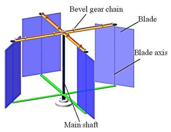
Figure 1.
Three-dimensional model of a VAWT.

Table 1.
Parameters of the 2D variable-pitch vertical-axis wind turbine.
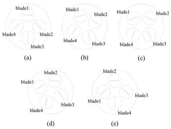
Figure 2.
The position of the blade at different times. (a) t = 0, (b) t = 1/8 T, (c) t = 1/4 T, (d) t = 3/8 T, (e) t = 1/4 T.
3. Calculation Method
3.1. Computational Domain and Boundary Conditions
The computational domain, as shown in Figure 3, is divided into three regions. The external region is a stationary region without rotation, the region containing the wind turbine is the revolution zone, and the region containing the four blades is the rotation zone. The dimensions of the computational domain are 12 m in length and 6 m in width, with the center of the rotation zone located 3 m away from the left inlet in the horizontal direction and 3 m away from the top and bottom inlets in the vertical direction.
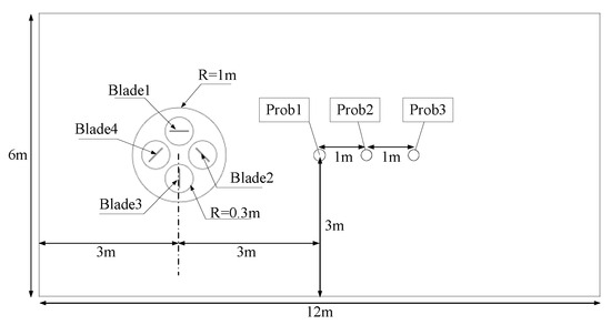
Figure 3.
Computational domain.
The boundary conditions are set as shown in Figure 4. The left and top/bottom boundaries are velocity inlets with the X direction being the inflow direction. The right boundary is a pressure outlet with a pressure value of 101,325 Pa. The surfaces representing the vanes are set as no-slip walls. Under uniform inflow conditions, the inflow velocity is 6 m/s. Under fluctuating inflow conditions, the wind speed is modeled as a sinusoidal function over time, expressed as follows:
where is the inflow velocity, denotes the mean velocity, is the velocity amplitude, is the fluctuating wind frequency, and represents time. The fluctuating wind we studied is different from turbulent wind and can only be simulated in a laboratory or computer environment. Our objective is to investigate the influence of various fluctuating wind parameters, such as frequency and amplitude, on the aerodynamic performance of VAWTs. Similar methods for simulating fluctuating inflow are employed in references [17,18].
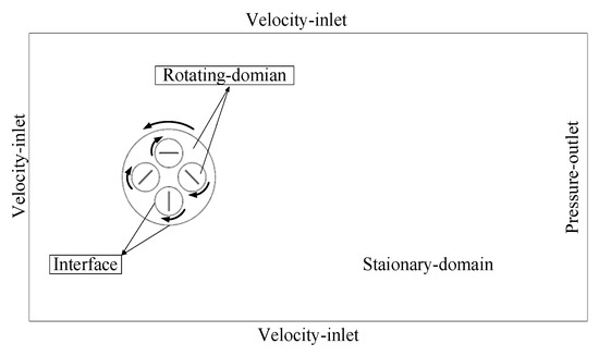
Figure 4.
Boundary conditions setting for the flow field.
3.2. Grid Generation
Structured grids are used in all regions with appropriate refinements in the two rotation regions and the wake region to ensure the accurate simulation of the flow state, as shown in Figure 5 (The black arrow indicates the local magnification). The turbulence model requires the first layer of wall-adjacent grid cells to satisfy 30 < y+ < 300, with the first grid point located at roughly from the wall. The rotation regions are treated using the Multiple Reference Frames (MRF) approach, and the interface between the outer rectangular region and the central circular region as well as that between the rotation region and the revolution region are both set as interface boundaries.
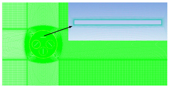
Figure 5.
Computational grid.
3.3. Solution Method
The control equations comprise the continuity equation and the momentum equation for incompressible flow:
In the equation, represents the time-averaged velocity in direction i, represents Reynolds stress, represents air density, represents the pressure on the fluid element, and represents the dynamic viscosity.
Ansys Fluent 2021r2 is used for calculations. The widely used model is selected for the turbulence model. The SIMPLE algorithm is used for solving the coupling of velocity and pressure, and the QUICK scheme and second-order upwind scheme are used for discretization of convective and diffusion terms of the governing equations, respectively. First-order implicit scheme are used to discretise non-stationary terms. We noticed that many references used a wind turbine rotation angle of 1° or 2° for each time step. We employed a time step of 0.001 s, corresponding to a wind turbine rotation angle of approximately 0.206°, which enhances the accuracy of the calculations. The convergence criterion is set to . Our simulations were conducted on an Intel(R) Xeon(R) Gold 5218R processor with a CPU clock speed of 2.1 GHz and 64 GB of RAM, utilizing two processor cores. The computation took approximately 8 h (equivalent to a physical flow time of 8 s, approximately 4.58 wind turbine rotation cycles).
3.4. Proper Orthogonal Decomposition (POD)
For the flow field variable (e.g., velocity or pressure), N discrete sequence data , referred to as “snapshots” or samples, are selected [22]. The principle of the POD method is to rapidly decay the projection components of the sample data on the orthogonal basis, such that the projection component on the current orthogonal basis achieves the maximum [23,24]:
Equation (4) can be transformed into a maximum eigenvalue problem:
The POD basis functions are defined as follows:
Substituting Equation (6) into the equation, the following formula can be written:
The column vector represents the eigenvectors corresponding to the eigenvalues of the matrix . These eigenvalues represent the energies on the corresponding basis functions, and their sum represents the total energy of the system.
In general, the eigenvalue sequence decays rapidly, and the first few POD bases usually contain more than 90% of the flow field energy. Therefore, for complex systems, extracting a certain number of snapshots for POD analysis and analyzing a few dominant POD bases can reveal to a large extent the system’s main characteristics [25,26,27].
By selecting the first M (M < N) POD bases and representing the flow field variables with the basis functions, an approximation of the original samples can be obtained:
4. Numerical Method Validation
For grid independence, the numerical simulation is carried out with the uniform flow of 6 m/s, the rotation angular velocity of the fan is 3.6 rad/s, and the rotation angular velocity of the blade is −1.8 rad/s. Under the premise of not changing the grid generation strategy, three grid dimensions are considered with the grid numbers being 58,343, 100,253, and 143,776, respectively. The X-component velocity at the point Prob1 in Figure 3 was monitored, and the results obtained with the three grid quantities between 4 s and 6 s were compared, as shown in Figure 6a. The results show that the result derived by the grid with 58,343 cells had significant deviation from the results with 100,253 and 143,776 grid cells. On the other hand, the difference between the result with 100,253 cells and that with 143,776 cells is nearly negligible. Therefore, the grid with 100,253 cells was selected for subsequent numerical simulations. After a computational time equivalent to two 1/4 wind turbine cycles (0.872 s), the flow field reaches a pseudo-stationary state.
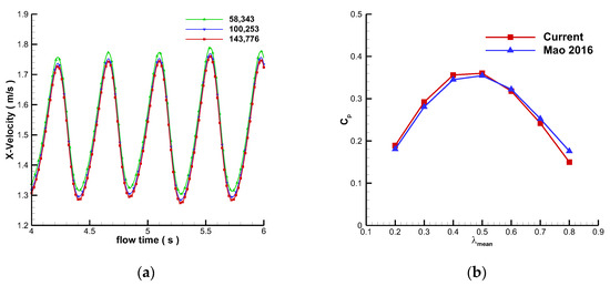
Figure 6.
Numerical validation. (a) comparison of X-component velocities at Prob1 with different grid numbers; (b) Comparison with the results in reference [12].
The average of the blades is given by
where represents the angular velocity of the wind turbine, is the radius of the wind turbine, and is the mean inflow velocity.
The power coefficient is defined as
and it is related to the torque coefficient by
The method for time-averaged the computational variable C is as follows:
We compared our curves with results from [12], as illustrated in Figure 6b. The results from both studies are in substantial agreement.
5. Results and Discussion
5.1. Flow Characteristics Analysis
In this section, the selected uniform inflow velocity is 6 m/s. For the fluctuating wind inflow condition, the parameters are as follows: and . The angular velocity of the rotation domain is 3.6 rad/s, and the angular velocity of the blade’s rotation is −1.8 rad/s.
To analyze the flow characteristics of the wind turbine under different flow conditions, the velocity variations at different points in the wake of the wind turbine are monitored, as shown in Figure 3. The widely used Q criterion [28] is used for vortex identification, which is derived from the second invariant of the velocity gradient tensor:
where A and B are the Helmholtz velocity decompositions of the velocity gradient tensor, and the regions with Q > 0 denote the presence of vortex structures. Figure 7 shows the vortices during a fluctuating cycle from 4 s to 6 s under the two inflow conditions. It can be observed that the vortices under both inflow conditions are closely distributed near the blades, and the alternating shedding vortices appear in the wake region behind the rotor, forming a von Kármán vortex street. The rotation of the wind turbine leads to the asymmetry of the von Kármán vortex street, with counterclockwise rotation resulting in a higher concentration of vortex cores on the upper windward side of the wind turbine.
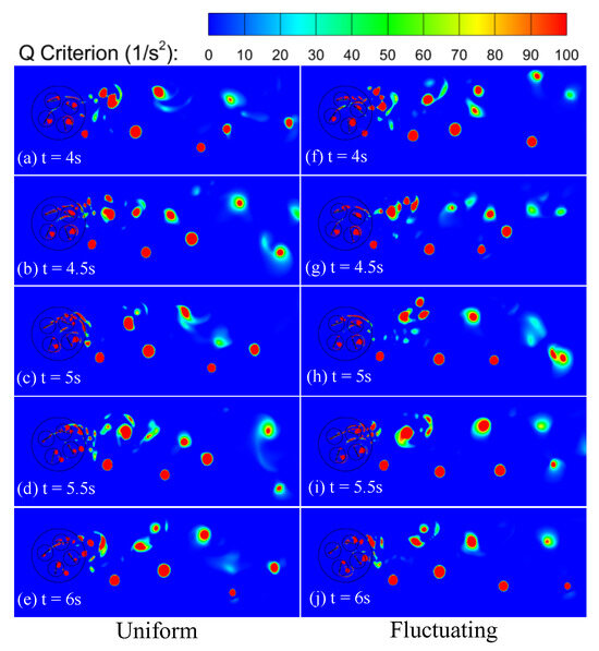
Figure 7.
Q-criterion contours at different time steps for two inflow conditions.
FFT is applied to the velocity at each point to obtain different frequency components of the flow field. The power spectra plots are shown in Figure 8. Figure 8a shows the power spectrum for uniform inflow condition. From Figure 8a, it can be observed that in the case of uniform inflow, there is only one dominant frequency in the flow field, which is 2.29 . According to , the frequency corresponds to the rotational frequency of the wind turbine of 3.6 rad/s. Figure 8b shows the power spectrum for fluctuating inflow condition. It can be clearly seen that in this case, there are two dominant frequencies, which are 0.5 and 2.29. The frequency of 2.29 corresponds to the rotation frequency of the wind turbine, while the value 0.5 corresponds to the frequency of the fluctuating inflow.
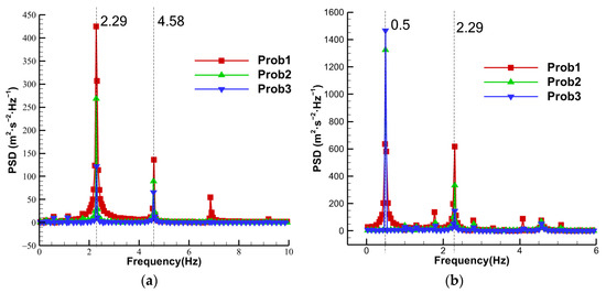
Figure 8.
Power spectral density (PSD) for different inflow conditions. (a) Uniform inflow. (b) Fluctuating wind inflow.
5.2. Influence of Fluctuating Wind Amplitude
To investigate the effect of fluctuating wind amplitude on the performance of the variable-pitch VAWT, the inflow frequency was kept at with a mean tip speed ratio . The amplitude of the fluctuating wind varied from 10% to 50% of the mean speed . Figure 9 shows the variation in the tip speed ratio with time for different amplitudes. It can be observed that smaller amplitudes result in a narrower fluctuation range of , with a maximum difference of 0.4 and a minimum difference of 0.06.
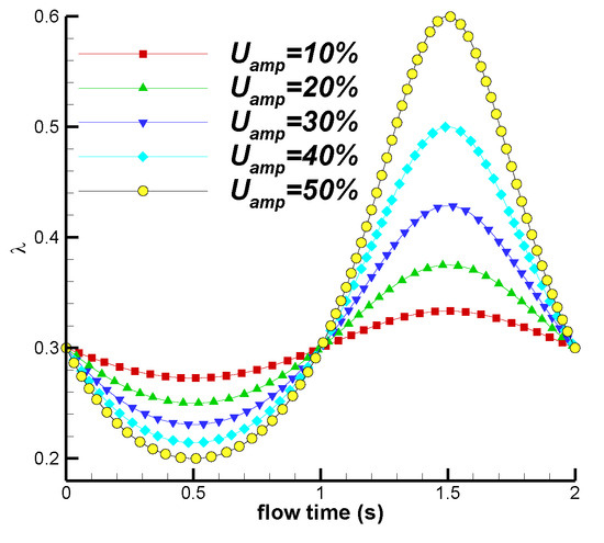
Figure 9.
Variation in with different fluctuating amplitudes.
Figure 10 shows the variations in the inflow velocity with different amplitudes during the time interval from 3.5 s to 5.5 s. The fluctuating wind cycle is 2 s, and the rotation cycle of the wind turbine is 1.745 s, corresponding to a rotation angle of per fluctuating cycle. From 3.5 s to 4 s, the inflow velocity is lower than the mean inflow velocity , with larger amplitudes resulting in lower velocity values. From 4 s to 5 s, the incoming flow velocity is higher than the mean inflow velocity, with larger amplitudes corresponding to higher velocity values.
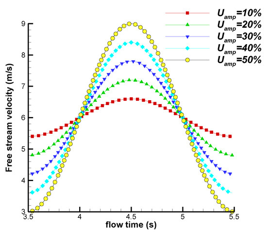
Figure 10.
Velocity variation within one fluctuating cycle.
Figure 11 shows the variation in the torque coefficient for the wind turbine under different amplitudes (10%, 30%, 40%, 50%) within one fluctuating cycle. The torque coefficient is defined as follows:
where M is the total torque of the four blades, and is the air density. In addition, is the swept area of the inflow, which is defined as follows:
where and represent the blade chord length and thickness, respectively (). It can be observed that the peak value of the curve increases as the inflow amplitude increases. As the wind turbine rotates from the phase angle of 0 to , i.e., from 3.5 s to 3.94 s, the torque first increases, then decreases, and then increases again, showing both maximum and minimum values. From 3.94 s to 4.38 s, as the wind turbine rotates from to , the torque follows a similar trend. The torque curve changes in the same way within each 1/4 cycle. This is because the angular velocity of the variable-pitch wind turbine is twice the angular velocity of the blade, which means that the blade position is the same as the initial position after each 1/4 cycle.
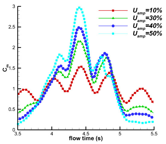
Figure 11.
Variations in torque coefficient with different amplitudes.
Figure 12 shows the variation in the torque coefficient of each blade within a fluctuating cycle with . It can be observed that when the wind turbine reaches the initial position (Figure 2a), the torque magnitudes of the blades follow the order , where represents the torque of the blade with index i. When the wind turbine rotates for 1/4 cycle, blade 1 reaches the position of blade 4 at the initial moment, resulting in torque magnitudes following the order . Within each 1/4 cycle, one blade reaches its peak torque, and the torques of the four blades sequentially peak within one fluctuating cycle.
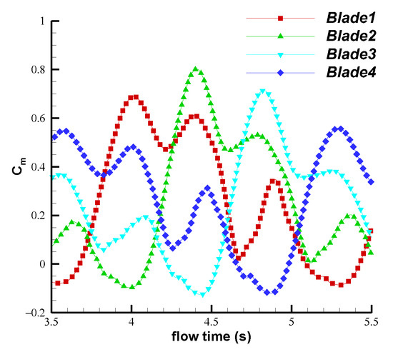
Figure 12.
Variations in torque coefficients for individual blades under .
Figure 13 illustrates the variation in the power coefficient within a fluctuating cycle under different amplitude conditions. As seen from Figure 13, it can be observed that the power coefficient does not become negative for larger fluctuating amplitudes, indicating that the performance of the variable-pitch VAWT remains favorable under high-amplitude fluctuating conditions.
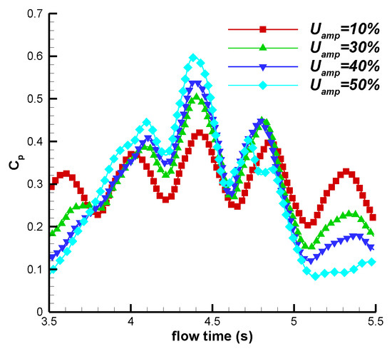
Figure 13.
Variations in power coefficients under different amplitudes.
Table 2 shows the time averaged torque coefficient and power coefficient with different amplitude conditions (where the amplitude of 0 corresponds to a uniform inflow). It can be seen that the time-averaged torque coefficient increases as the inflow amplitude increases, and the time-averaged torque coefficients under fluctuating conditions are greater than that under uniform wind conditions. For fluctuating amplitudes ranging from 30% of to 50% of , the time-averaged power coefficient is greater than that under uniform wind conditions.
Table 2.
Time-averaged power coefficient and torque coefficient with different amplitudes.
5.3. Influence of Fluctuating Wind Frequency
To investigate the effect of frequency on the performance of the variable-pitch VAWT, the mean tip speed ratio was fixed as 0.3, while the amplitude was set to 30% of . The fluctuating frequency was set to , , , and . The rotation angular velocity of the rotating domain was 3.6 rad/s, and the rotation angular velocity of the blade was −1.8 rad/s.
Figure 14 shows the variation in the inflow velocity with time for different frequencies. The average inflow velocity under fluctuating conditions was 6 m/s, with maximum and minimum inflow velocities of 7.8 m/s and 4.2 m/s, respectively, resulting in a peak-to-peak difference of 3.6 m/s. The maximum cycle of the fluctuating wind was 4 s, while the minimum cycle was 1.182 s. Figure 15 shows the variation in the tip speed ratio for different frequencies. The maximum and minimum values of were 0.43 and 0.23, respectively, with a peak-to-peak difference of 0.20. Different frequencies of the inflow result in different turbine rotation angles within a fluctuating cycle, as shown in Table 3.
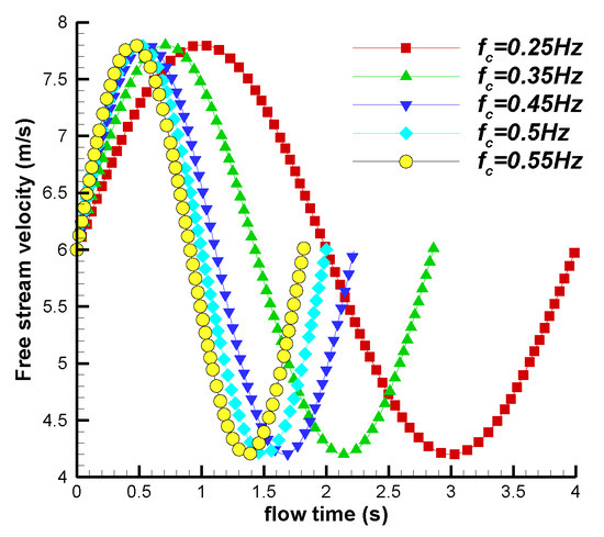
Figure 14.
Wind velocity variation in inflow with different frequencies.
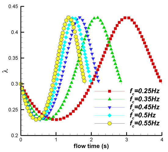
Figure 15.
Variations in tip speed ratios with different frequencies.
Table 3.
Time-averaged torque coefficient and power coefficient with different frequencies.
Figure 16 shows the torques with the frequency values of , , and . The time interval for analysis was from 1.744 s to 3.744 s after the flow reached a stable state. It can be observed that the torque curve of the wind turbine varied with the inflow velocity. Starting from the initial position, the torque of the wind turbine increases first, then decreases and then increases again within each 1/4 cycle. The average torque with was the smallest and that with was the largest. Figure 17 shows the power coefficient curves with frequencies of , and . It can be observed that the average power coefficient with was the smallest and that with was the largest.
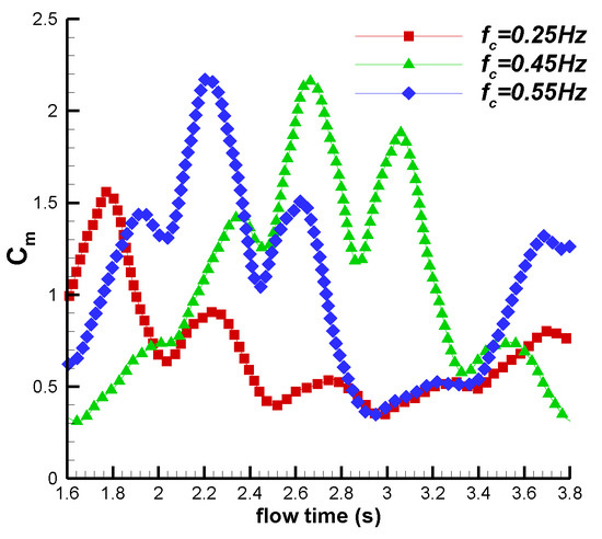
Figure 16.
Variations in torque coefficients with different frequencies.
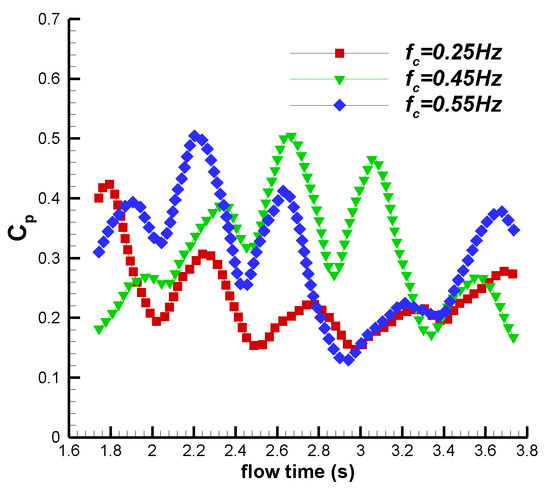
Figure 17.
Variations in power coefficients with different frequencies.
Table 3 shows the time-averaged total torque and power coefficient with different frequencies within 2 s. From Table 3, it can be observed that for , the time-averaged torque and power coefficient increased with the increase in frequency, with maximum values of 1.122 and 0.323, respectively. However, for , the time-averaged torque and power coefficient decreased with the increase in frequency.
5.4. Influence of Average Tip Speed Ratio
To study the effect of the mean tip speed ratio under fluctuating wind conditions, the parametersand 30% were kept. The average tip speed ratio of the wind turbine varied from to 0.8, and the power coefficient was analyzed for each case.
Figure 18 shows the variations in the tip speed ratios with time with different mean tip speed ratios. At the maximum mean tip speed ratio , the maximum tip speed ratio was 1, and the minimum tip speed ratio was 0.54, resulting in a peak-to-peak difference of 0.46. For the minimum mean tip speed ratio , the maximum and minimum tip speed ratios were 0.429 and 0.231, respectively, with a peak-to-peak difference of 0.198.
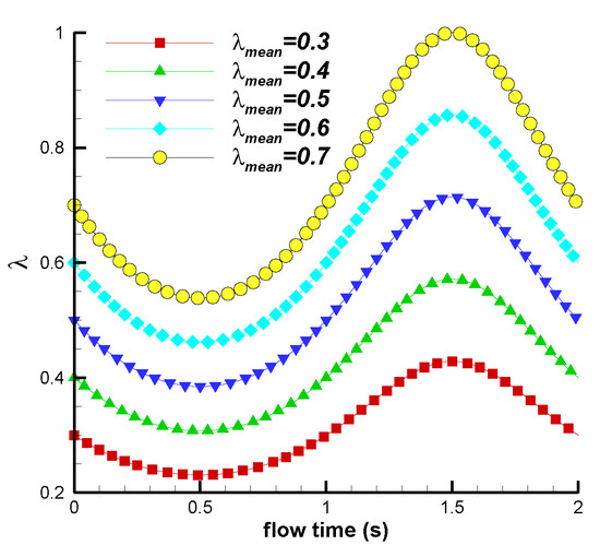
Figure 18.
Variation in tip speed ratio with time.
Figure 19 shows the variations in the torque coefficients with different mean tip speed ratios over time. The wind turbine speed and the number of wind turbine rotor revolutions within a fluctuating cycle increase as increases. As the mean tip speed ratio increases, the torque coefficient curve is shifted downward as the wind turbine speed increases, shortening the cycle. A torque peak occurs within each 1/4 cycle, and the number of torque peaks within a fluctuating cycle increases with the mean tip speed ratio. Considering Figure 18 and Figure 19, it can be observed that in the first half of the fluctuating cycle (2 s to 3 s), the tip speed ratio was lower than the mean tip speed ratio, and the inflow velocity was higher than the mean flow velocity. In the second half of the cycle (3 s to 4 s), the tip speed ratio was higher than the mean tip speed ratio, and the inflow speed was lower than the mean flow velocity. The torque values in the first half of the cycle were greater than those in the second half. In the second half, the torque coefficient decreases significantly as reaches its peak. Within a fluctuating cycle, the maximum torque coefficient decreases as the mean tip speed ratio increases.
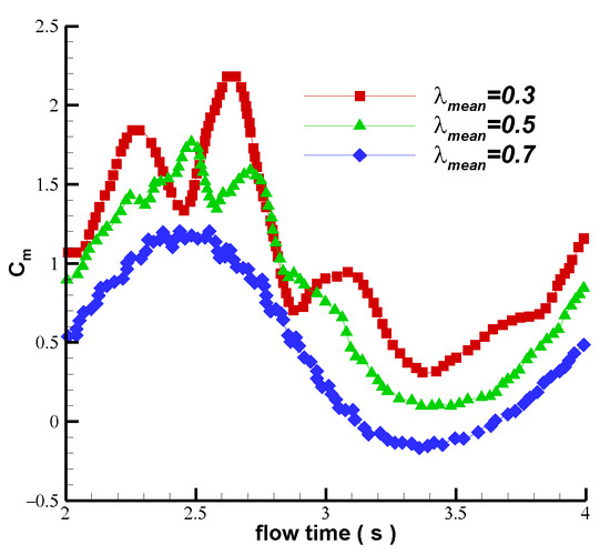
Figure 19.
Variations in torque coefficients with different mean tip speed ratios.
Figure 20 shows the variations in the power coefficients with different average tip speed ratios. It can be observed that under fluctuating wind conditions, when the mean tip speed ratio was relatively high (0.7), the power coefficient of the variable-pitch VAWT exhibits negative values for certain cycles of time, indicating a reduced turbine performance.
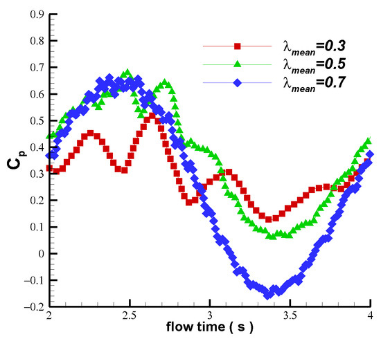
Figure 20.
Variations in power coefficients with different .
Figure 21 shows the time-averaged torque coefficient under fluctuating and uniform wind conditions with different tip speed ratios. From Figure 21, it can be seen that regardless of the magnitude of the tip speed ratio, the torque coefficient under fluctuating wind conditions was always greater than that under uniform wind conditions. When , the torque increases as the mean tip speed ratio increases. When , the torque reaches its maximum value, with maximum values of 1.054 for fluctuating wind and 0.994 for uniform wind. When , the torque decreases as the mean tip speed ratio increases.
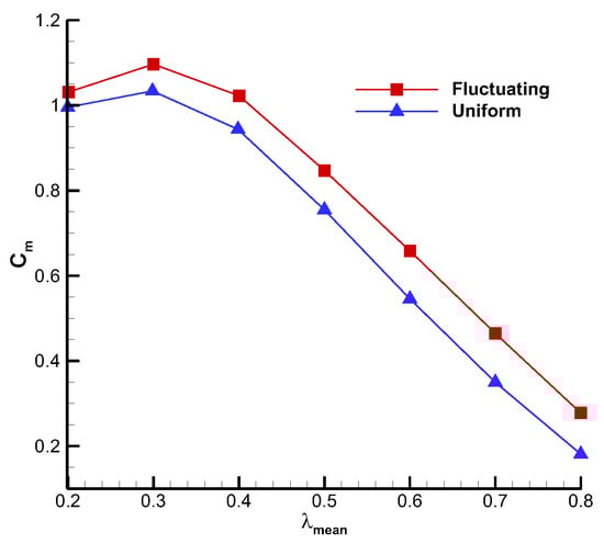
Figure 21.
Time-averaged torque coefficients with different wind conditions.
Figure 22 shows the time-averaged power coefficient under fluctuating and uniform inflow conditions with different mean tip speed ratios. It can be observed that when the mean tip speed ratio was relatively low ( is between 0.2 and 0.4), the power coefficients with both inflow conditions increases with the increase of . At 0.5, the power coefficient reaches its maximum value, with maximum values of 0.372 for fluctuating wind (about 2.2 times that of the unmodified Savonius wind turbine [29,30]) and 0.363 for uniform wind. When 0.5, the power coefficients decrease as the mean tip speed ratio increases, and the power coefficient under fluctuating wind conditions was always greater than that under uniform wind conditions.
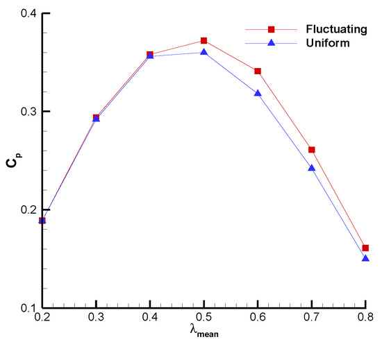
Figure 22.
Time-averaged power coefficients under different wind conditions.
The influences of the average tip speed ratio on the torque and power coefficient of the variable-pitch VAWT are not entirely consistent. For a relatively low , the torque experienced by the wind turbine is greater, but the power coefficient is lower. Conversely, when the mean tip speed ratio is high and the power coefficient is high, the total torque of the wind turbine may be quite small. Therefore, selecting an appropriate is essential to achieve an optimal aerodynamic performance. In terms of wind energy capture, a mean tip speed ratio close to 0.5 is preferred.
5.5. POD Analysis
In this section, POD analysis is performed to analyze the flow characteristics for two different inflow conditions: uniform inflow at 6 m/s and fluctuating inflow with , and . The data sets for the uniform inflow case were taken from snapshots of velocity fields with a time interval of 0.002 s within t = 2 s~2.436 s (corresponding to one wind turbine rotation cycle), containing a total of 218 instantaneous velocity fields. For the fluctuating inflow case, the data sets were taken with a time interval of 0.08 s within t = 2 s~30 s (including 64 turbine rotation cycles and 14 fluctuating wind cycles), containing a total of 350 velocity fields.
Following the approach described in Section 3.4, POD analysis was performed on both data sets. Figure 23 shows the frequency domain plots obtained by applying FFT to the POD coefficients for the two cases. It is shown that for the uniform inflow case, the POD coefficients have a frequency of 2.29 . For the fluctuating inflow case, the POD coefficients exhibit frequencies of 0.50 and 2.29 , consistent with the results in Section 5.1. This also indicates that there is no frequency locking phenomenon between the frequency of incoming wind and the rotational frequency of the wind turbine.
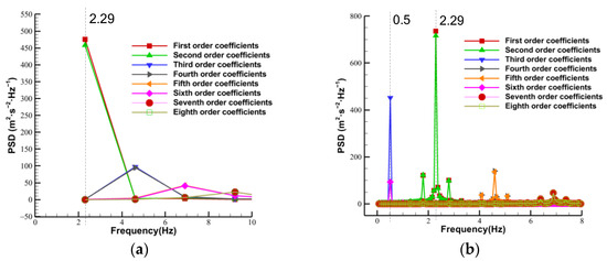
Figure 23.
Frequency domain representations of different POD coefficients for uniform wind (a) and fluctuating wind (b).
The energy distributions of the POD bases for both inflow conditions are shown in Figure 24. It can be observed that the energy distribution is more scattered for the fluctuating inflow compared to the uniform inflow. Under uniform inflow conditions, the first two POD modes capture most of the information of the flow field, accounting for 94.79% of the total energy. However, under fluctuating inflow conditions, the first two modes accounted for only 80.15% of the total energy. To achieve a close energy (99.6%) capture as the uniform inflow, the first 12 modes were required for the fluctuating inflow case, while only the first six modes were required for the uniform inflow case. The fact that the energy distribution is more dispersed for the fluctuating inflow indicates that more POD bases are needed for flow field reconstruction compared to the uniform inflow case.
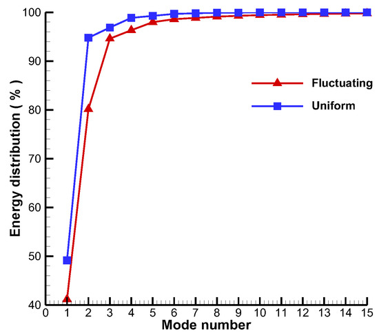
Figure 24.
Variations in energy distributions for the two inflow cases.
Figure 25 and Figure 26 show the contours of the X and Y components of each POD mode for both inflow conditions. It can be observed that the flow field under the fluctuating inflow is more dispersed and complex compared to that under the uniform inflow. In both cases, the POD modes appear in pairs, and the vortex distribution of the second mode is mainly in the interphase of the vortex distribution of the first mode. They are added up to reconstruct the original flow field. As the wind turbine rotates counterclockwise, the vortex structures in each POD mode tend to be biased toward the windward side of the wind turbine, indicating that the areas with relatively large vortex amplitudes correspond to the windward side of the wind turbine. In the regions near the blades, there are numerous rapidly shedding vortex structures. As the inflow passes through the blades, it is sheared by the cutting action of the blades, resulting in flow separation. This creates strong rotational flow disturbances at the blade tips. As the distance from the wind turbine increases, the vortices become larger, and the velocity gradually decreases. This implies that the turbulence is stronger near the wind turbine when it is operated, and the turbulence intensity increases as the distance from the wind turbine decreases. These results are in agreement with the findings of Araya et al. [31].
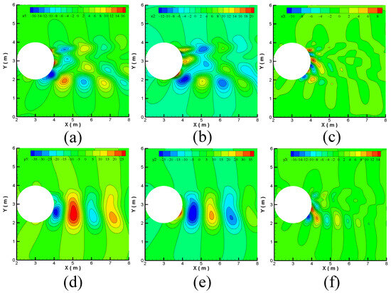
Figure 25.
Contours of POD modes for uniform inflow conditions. (a) Mode 1 . (b) Mode 2 . (c) Mode 3 . (d) Mode 1 . (e) Mode 2 . (f) Mode 3 .
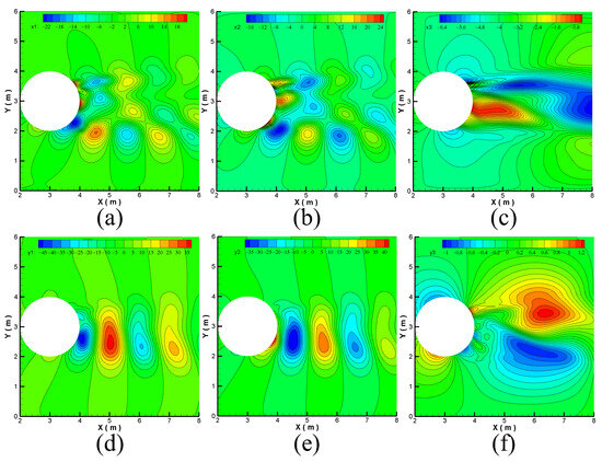
Figure 26.
Contours of POD modes for fluctuating wind conditions. (a) Mode 1 . (b) Mode 2 . (c) Mode 3 . (d) Mode 1 . (e) Mode 2 . (f) Mode 3 .
Figure 27 shows a comparison of the instantaneous X-component velocity fields reconstructed by the first six POD modes for uniform inflow and the first 12 POD modes for fluctuating inflow with the original (CFD) flow fields. It can be seen that the reconstructed flow fields using POD modes match closely with the original flow field for both inflow conditions. Due to the complexity of the fluctuating inflow, the error for the fluctuating inflow is slightly larger than that for the uniform inflow.
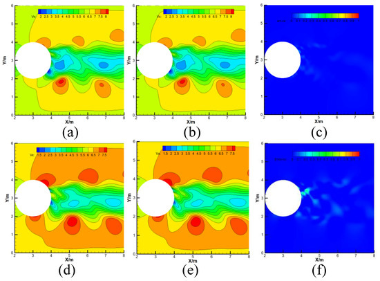
Figure 27.
POD-based reconstruction of instantaneous X-component velocity fields compared with the original flow fields. (a) Original flow field for uniform wind conditions. (b) Reconstruction with the first six POD modes for uniform wind flow. (c) Reconstruction error for uniform wind flow. (d) Original flow field for fluctuating wind conditions. (e) Reconstruction with the first 12 POD modes for fluctuating wind flow. (f) Reconstruction error for fluctuating wind conditions.
6. Conclusions
This study analyzes the aerodynamic performances of a variable-pitch VAWT under fluctuating inflow conditions with different amplitudes, frequencies, and mean tip speed ratios and compares them with the aerodynamic performances under uniform inflow conditions. In addition, the flow fields for both inflow conditions are decomposed and reconstructed using the POD method. The following conclusions are drawn:
In the case of relatively large amplitudes (30–50%) under fluctuating inflow conditions, the power coefficients of the wind turbine are higher than that under uniform inflow conditions.
As the inflow frequency increases, the torque coefficient and power coefficient of the turbine first increase and then decrease, reaching their maximum values at an inflow frequency of .
The torque coefficients of the turbine under fluctuating inflow conditions are consistently higher than those under uniform inflow conditions as varies.
At a relatively low , the turbine experiences a higher torque but a lower power coefficient. Conversely, a higher power coefficient may result in a lower total torque. Therefore, a tip speed ratio close to 0.5 is preferable for good aerodynamic performances.
The energy distribution under the fluctuating inflow condition is more dispersed than that under the uniform inflow condition. Under the uniform inflow condition, the first two POD modes sufficiently represent most of the flow characteristics. While under the fluctuating inflow condition, up to the first six POD modes are required to capture most of the flow characteristics.
Multiple directions have been identified for continuing the work presented in this paper. The work of this study is based on two-dimensional simulation. The existing literature [18] and results of this study indicate that two-dimensional analysis overpredicted the efficiency compared to three-dimensional analysis. Three-dimensional analysis is essential as it accounts for end effects and strong interactions between the trailing vortices and the following blade. Three-dimensional simulations will be pursued in the future. In addition, dynamic stall is a common phenomenon that appears mainly on rotating rotor blades, and it becomes one of the most limiting factors of the aerodynamic performance [32]. This phenomenon has a significant influence on the VAWT and could be investigated in future work. Mounting a Gurney flap at the trailing edge of the blade increases the power production of the turbine considerably [33]. Pitch effects combined with add-ons, such as Gurney flaps, are also new directions of research.
Author Contributions
W.Z. and S.Y. conceived the study and performed the simulations. W.Z. and C.C. wrote the paper. L.L. reviewed and edited the manuscript. All authors have read and agreed to the published version of the manuscript.
Funding
This research was supported by the National Science Foundation of China (Grant No. 11902278), State Key Laboratory of Aerodynamics, and the GHfund A (202302015072).
Data Availability Statement
The data presented in this study are available upon request from the corresponding author.
Conflicts of Interest
The authors declare no conflict of interest.
References
- Liao, L.; Ling, Y.; Huang, B.; Zhou, X.; Luo, H.; Xie, P.; Wu, Y.; Huang, J. Toward a Survey-Based Assessment of Wind Turbine Noise: The Impacts on Wellbeing of Local Residents. Energies 2020, 13, 5845. [Google Scholar] [CrossRef]
- Stevens, R.J.A.M.; Meneveau, C. Flow Structure and Turbulence in Wind Farms. Annu. Rev. Fluid Mech. 2017, 49, 311–339. [Google Scholar] [CrossRef]
- Gerrie, C.; Islam, S.Z.; Gerrie, S.; Turner, N.; Asim, T. 3D CFD Modelling of Performance of a Vertical Axis Turbine. Energies 2023, 16, 1144. [Google Scholar] [CrossRef]
- Michna, J.; Rogowski, K. CFD Calculations of Average Flow Parameters around the Rotor of a Savonius Wind Turbine. Energies 2022, 16, 281. [Google Scholar] [CrossRef]
- Villeneuve, T.; Boudreau, M.; Dumas, G. Improving the Efficiency and the Wake Recovery Rate of Vertical-Axis Turbines Using Detached End-Plates. Renew. Energy 2020, 150, 31–45. [Google Scholar] [CrossRef]
- Mejia, O.; Quiñones, J.; Laín, S. RANS and Hybrid RANS-LES Simulations of an H-Type Darrieus Vertical Axis Water Turbine. Energies 2018, 11, 2348. [Google Scholar] [CrossRef]
- Liu, L.; Liu, C.; Zheng, X. Modeling, Simulation, Hardware Implementation of a Novel Variable Pitch Control for H-Type Vertical Axis Wind Turbine. J. Electr. Eng. 2015, 66, 264–269. [Google Scholar] [CrossRef]
- Elkhoury, M.; Kiwata, T.; Aoun, E. Experimental and Numerical Investigation of a Three-Dimensional Vertical-Axis Wind Turbine with Variable-Pitch. J. Wind Eng. Ind. Aerodyn. 2015, 139, 111–123. [Google Scholar] [CrossRef]
- Zhang, L.; Zhang, S.; Wang, K.; Liu, X.; Liang, Y. Study on Synchronous Variable-Pitch Vertical Axis Wind Turbine. In Proceedings of the 2011 Asia-Pacific Power and Energy Engineering Conference, Wuhan, China, 25–28 March 2011; pp. 1–5. [Google Scholar]
- Sagharichi, A.; Maghrebi, M.J.; ArabGolarcheh, A. Variable Pitch Blades: An Approach for Improving Performance of Darrieus Wind Turbine. J. Renew. Sustain. Energy 2016, 8, 053305. [Google Scholar] [CrossRef]
- Aliferis, A.D.; Jessen, M.S.; Bracchi, T.; Hearst, R.J. Performance and Wake of a Savonius Vertical-axis Wind Turbine under Different Incoming Conditions. Wind Energy 2019, 22, 1260–1273. [Google Scholar] [CrossRef]
- Mao, Z.; Tian, W.; Yan, S. Influence Analysis of Blade Chord Length on the Performance of a Four-Bladed Wollongong Wind Turbine. J. Renew. Sustain. Energy 2016, 8, 023303. [Google Scholar] [CrossRef]
- Elgendi, M.; AlMallahi, M.; Abdelkhalig, A.; Selim, M.Y.E. A Review of Wind Turbines in Complex Terrain. Int. J. Thermofluids 2023, 17, 100289. [Google Scholar] [CrossRef]
- Cheng, S.; Elgendi, M.; Lu, F.; Chamorro, L.P. On the Wind Turbine Wake and Forest Terrain Interaction. Energies 2021, 14, 7204. [Google Scholar] [CrossRef]
- Wu, Z.; Bangga, G.; Cao, Y. Effects of Lateral Wind Gusts on Vertical Axis Wind Turbines. Energy 2019, 167, 1212–1223. [Google Scholar] [CrossRef]
- Danao, L.A.; Eboibi, O.; Howell, R. An Experimental Investigation into the Influence of Unsteady Wind on the Performance of a Vertical Axis Wind Turbine. Appl. Energy 2013, 107, 403–411. [Google Scholar] [CrossRef]
- Wekesa, D.W.; Wang, C.; Wei, Y.; Danao, L.A.M. Influence of Operating Conditions on Unsteady Wind Performance of Vertical Axis Wind Turbines Operating within a Fluctuating Free-Stream: A Numerical Study. J. Wind Eng. Ind. Aerodyn. 2014, 135, 76–89. [Google Scholar] [CrossRef]
- Bhargav, M.M.S.R.S.; Ratna Kishore, V.; Laxman, V. Influence of Fluctuating Wind Conditions on Vertical Axis Wind Turbine Using a Three Dimensional CFD Model. J. Wind Eng. Ind. Aerodyn. 2016, 158, 98–108. [Google Scholar] [CrossRef]
- Mantravadi, B.; Unnikrishnan, D.; Sriram, K.; Mohammad, A.; Vaitla, L.; Velamati, R.K. Effect of Solidity and Airfoil on the Performance of Vertical Axis Wind Turbine under Fluctuating Wind Conditions. Int. J. Green Energy 2019, 16, 1329–1342. [Google Scholar] [CrossRef]
- Gharaati, M.; Xiao, S.; Wei, N.J.; Martínez-Tossas, L.A.; Dabiri, J.O.; Yang, D. Large-Eddy Simulation of Helical- and Straight-Bladed Vertical-Axis Wind Turbines in Boundary Layer Turbulence. J. Renew. Sustain. Energy 2022, 14, 053301. [Google Scholar] [CrossRef]
- Cooper, P.; Kennedy, O.C. Development and Analysis of a Novel Vertical Axis Wind Turbine; University of Wollongong: Wollongong, NSW, Australia, 2004. [Google Scholar]
- Sirovich, L.; Kirby, M. Low-Dimensional Procedure for the Characterization of Human Faces. J. Opt. Soc. Am. A 1987, 4, 519. [Google Scholar] [CrossRef]
- Zhang, W.; Chen, C. Global Stability Analysis of Flow Past Two Side-by-Side Circular Cylinders at Low Reynolds Numbers by a POD-Galerkin Spectral Method. Chin. Phys. Lett. 2012, 29, 084701. [Google Scholar] [CrossRef]
- Zhang, W.; Chen, C. Numerical simulation of flow around two side-by-side circular cylinders at low Reynolds numbers by a POD-Galerkin spectral method. Chin. J. Hydrodyn. 2009, 244, 463–471. [Google Scholar] [CrossRef]
- Zhao, M.; Zhao, Y.; Liu, Z.; Du, J. Proper Orthogonal Decomposition Analysis of Flow Characteristics of an Airfoil with Leading Edge Protuberances. AIAA J. 2019, 57, 2710–2721. [Google Scholar] [CrossRef]
- Zhou, T.; Yan, B.; Yang, Q.; Hu, W.; Chen, F. POD Analysis of Spatiotemporal Characteristics of Wake Turbulence over Hilly Terrain and Their Relationship to Hill Slope, Hill Shape and Inflow Turbulence. J. Wind Eng. Ind. Aerodyn. 2022, 224, 104986. [Google Scholar] [CrossRef]
- Stabile, G.; Hijazi, S.; Mola, A.; Lorenzi, S.; Rozza, G. POD-Galerkin Reduced Order Methods for CFD Using Finite Volume Discretisation: Vortex Shedding around a Circular Cylinder. Commun. Appl. Ind. Math. 2017, 8, 210–236. [Google Scholar] [CrossRef]
- Hunt, J.C.R.; Wray, A.A.; Moin, P. Eddies, Streams, and Convergence Zones in Turbulent Flows. Studying Turbulence using Numerical Simulation Databases; Proceedings of the 1988 Summer Program; Stanford University: Stanford, CA, USA, 1988; Volume 2, pp. 193–208. [Google Scholar]
- Irabu, K.; Roy, J.N. Study of Direct Force Measurement and Characteristics on Blades of Savonius Rotor at Static State. Exp. Therm. Fluid Sci. 2011, 35, 653–659. [Google Scholar] [CrossRef]
- Mao, Z.; Tian, W. Effect of the Blade Arc Angle on the Performance of a Savonius Wind Turbine. Adv. Mech. Eng. 2015, 7, 168781401558424. [Google Scholar] [CrossRef]
- Araya, D.B.; Colonius, T.; Dabiri, J.O. Transition to Bluff-Body Dynamics in the Wake of Vertical-Axis Wind Turbines. J. Fluid Mech. 2017, 813, 346–381. [Google Scholar] [CrossRef]
- Bangga, G.; Hutani, S.; Heramarwan, H. The Effects of Airfoil Thickness on Dynamic Stall Characteristics of High-Solidity Vertical Axis Wind Turbines. Adv. Theory Simul. 2021, 4, 2000204. [Google Scholar] [CrossRef]
- Chakroun, Y.; Bangga, G. Aerodynamic Characteristics of Airfoil and Vertical Axis Wind Turbine Employed with Gurney Flaps. Sustainability 2021, 13, 4284. [Google Scholar] [CrossRef]
Disclaimer/Publisher’s Note: The statements, opinions and data contained in all publications are solely those of the individual author(s) and contributor(s) and not of MDPI and/or the editor(s). MDPI and/or the editor(s) disclaim responsibility for any injury to people or property resulting from any ideas, methods, instructions or products referred to in the content. |
© 2023 by the authors. Licensee MDPI, Basel, Switzerland. This article is an open access article distributed under the terms and conditions of the Creative Commons Attribution (CC BY) license (https://creativecommons.org/licenses/by/4.0/).