Abstract
The third-order state observer implements the decoupled control and the accurate estimation of the d-axis current, q-axis current, and rotor speed of the permanent magnet synchronous motor (PMSM). Its complex calculation, however, is a challenge for most digital controllers in practical applications. The authors proposed an improved dual second-order observer based on the Kalman filter. A 0.88 Nm, 1500 rpm prototype was built. The simulation and experimental results prove the effectiveness and practicability of the proposed method.
1. Introduction
Thanks to its high transparency and high torque density, the compact, light, and thin drive unit is widely used in robot joints. It is composed of multiple pole-pair numbers and high torque density outer rotor motor [1] embedded in a planetary gearbox with low reduction ratio, which is also called a proprioceptive actuator [2], as shown in Figure 1. The highly integrated structure and multiple pole-pair numbers make the motor small in size but large in output torque. The planetary reduction gearbox with high reverse drive capability is used, which has the characteristics of high transparency and minimal nonlinear error, so that it can directly estimate the torque through the q-axis current [3]. It can realize high-precision force control without using an expensive torque sensor [4], saving a lot in costs. Because of its small size, low cost, and high torque density, this special structure has been gradually applied to multiple applications, such as mechanical arms, exoskeletons, automated guided vehicles (AGVs), and so on.
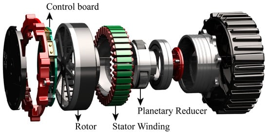
Figure 1.
Mechanical structure of proprioceptive actuator.
In order to reduce the cost of the low-power PMSM (e.g., several decades of watts), the three-phase currents are usually sampled by connecting the resistances in series with the lower bridge arms of the inverter [5]. The measurement accuracy is highly dependent on the accuracy of the resistance. As we all know, the value of the resistor changes with its temperature. As a robot joint, its use usually involves calculating the torque reference value based on the error between the reference speed and the actual measured speed, which requires a high-frequency calculation of the motor speed [6]. For the controller without a speed sensor and using the position information fed back by the encoder to calculate the speed, high measurement noise will be injected into the current loop, resulting in a large torque ripple [7]. It can be reduced by reducing the current and angle sensor noise, thereby achieving a higher precision force control. When there is no sensor, the state observer based on the state space model is an effective method to estimate the state variables. However, the system model inaccuracies and inevitable disturbances will cause a large deviation between the estimated value of the observer and the actual value. Therefore, a new state variable observation method is proposed; the estimated value of the observer and the measured value of the sensor are fused in some way.
The state space model is usually used to describe a system, which is generally expressed by differential equations [8]. In most control systems, when the state variables cannot be measured directly, the available system inputs and outputs are always used to estimate the state variables. This method of reconstructing the system state variables is called an observer [9,10]. At present, the popular observers include the slide mode observer (SMO), extended state observer (ESO), disturbance observer (DO), and Kalman observer (KO), etc.
SMO is insensitive to the changes of the model parameters and has strong robustness [7]. Some scholars have designed a full order slip film observer to estimate the flux and speed of the motor at the same time [11,12], in order to enhance the disturbance suppression ability of the speed loop. The ESO is robust to parameter variation, disturbance, and noise [13]. A traditional ESO is only used to estimate certain types of disturbances which have the same properties [14]. However, the actual PMSM system contains a variety of disturbances, such as the cogging torque, load torque, friction torque, measurement error effect, dead time effect, parameter disturbance, and other generalized disturbances [15]. As a result, a traditional ESO cannot suppress the impact of other types of disturbances on the system stability. In order to solve the above problems, Yan, Y. et al. proposed a full order extended state observer to estimate multiple disturbances [16,17], and designed a composite controller for compensation. Du, B. et al. embedded the position observer into the current controller [18]. The high-frequency current signal injection at a low speed and the extended electromotive force observer at a high speed are combined to form a hybrid position observer. For high-speed operation, a linear extended state observer (LESO) is used to replace the traditional synovial observer to reduce the observed speed jitter and phase delay. In order to improve the tracking performance of the current controller affected by internal disturbances such as parameter changes in the PMSM drive system, Qu L. et al. designed an extended state observer to estimate the internal disturbance of the PMSM in real time without establishing an accurate mathematical model [19]. And then used the estimated internal disturbance to update the control law of the sliding mode control in real time to improve the steady-state and transient current tracking performance, and enhanced the robustness to internal interference. The disturbance observer often uses the errors of the model and the actual system to inversely estimate the disturbance in the system [20]. Yi Y. et al. used it to estimate the load disturbance and its change rate to ensure that the speed tracking error converges to zero [21]. In order to improve the over-current protection and anti-interference performance of the PMSM system, some scholars have proposed a time-varying second-order nonlinear disturbance observer to estimate and compensate the motor parameter uncertainty and non-modeling dynamic disturbance, so as to eliminate the peak value of the initial time estimation [22]. The Kalman observer considers the system noise and measurement noise, and is usually used to fuse measurement data. According to the error correction between the state feedback value and the model prediction value, it achieves the best estimation of the state variables [23]. The Danish scholars Lund, S. h. J., and others, use the Kalman observer to estimate the q-axis current to reduce the measurement noise and improve the force control bandwidth [24,25]. At present, most research only focuses on the current loop or the speed loop, ignoring the coupling between the state variables of the current loop and the speed loop. For example, considering the angular velocity variable, which, coupled with the current variable, as a constant will lead to a large error in the estimated current value when the velocity ripples.
Usually, the d-axis current, q-axis current, and rotor mechanical angular velocity in the motor cannot be directly measured by sensors and are highly coupled with each other. To minimize the sensor measurement noise, realize the decoupling of the state variables, and reduce the computational burden of the digital control chip, the authors proposed a double second-order observer based on a double Kalman filter. By fusing the sensor-measured value, the accurate estimation of the current and angular velocity can be realized, respectively, and the purpose of reducing torque ripple can be achieved. Furthermore, to reduce the sensitivity of the observer to the motor parameters and the system model, this paper analyzed an improved strategy based on disturbance observation to improve the robustness of the observer.
2. Mathematical Model of PMSM
The mathematical model of PMSM can be divided into two sub models: the electrical model and mechanical model. The following assumptions and limitations are considered when establishing the electrical model and mechanical model:
- The stator windings are symmetrically distributed at an electrical angle of 120° in space, ignoring the spatial harmonics in the air gap;
- The air gap magnetoresistance has a constant component;
- Three phase sinusoidal voltage and corresponding winding balance;
- Hysteresis and eddy current are ignored.
2.1. Electrical Model
This paper takes the surface-mounted PMSM with a symmetrical rotor magnetic circuit as an example. Its d-axis inductance is equal to the q-axis inductance. For simplification, the voltage equations are converted into the d-q coordinate system, and are expressed as follows:
here, is the stator resistance, and are the inductance values of the d-axis and q-axis, and are the d-axis current and q-axis current, and are the voltage values of the d-axis and q-axis, is the electrical angular velocity of the motor rotor, and is the amplitude of the permanent magnet flux linkage.
2.2. Mechanical Model
The mechanical model is the equation of motion of the motor, involving force balance. The output torque of the motor is the electromagnetic torque, and is expressed as follows:
here, is the number of pole pairs.
For the surface-mounted PMSM, can be simplified as follows:
To operate at a given speed, the electromagnetic torque needs to overcome all torque components in opposite directions, including the load torque, friction torque, and the torque generated by the rotor and load inertia. According to the dynamic analysis, the mechanical motion is established as follows:
here, is the moment of inertia of the rotor and the load, in kg·m2, is the mechanical angular velocity of the rotor, in rad/s; is the load torque, in Nm, and is the friction coefficient, in Nm·rad−1 s.
The relationship between and is shown in (5).
3. Design of Third-Order Observer Based on Kalman filter
An observer is a method which can estimate the unmeasurable state variables of a system based on a known mathematic model. To ensure the estimation accuracy, the error between the measured value and the observer output value is used to correct the estimation of the state variables in the form of feedback. It means that the estimated value gradually becomes consistent with the real one when the error tends to zero, which indicates the obtained state variable estimation is reliable and accurate. Compared with the traditional low-pass filter without feedback correction, the control system has a lower delay and can accurately estimate the original state.
According to the electrical and mechanical models analyzed in the previous section, the d-axis and q-axis currents and the speed of the rotor are coupled to each other. It is unreasonable to regard any state variable as a constant value. Therefore, the third-order state space model should be designed to describe the motor system. Its continuous time state equation is given by the following:
From (6), is a nonlinear factor. To simplify the state space model, Equation (6) needs to be linearized, that is, to satisfy . According to the differential equation , Equation (6) is simplified as the following:
Discretizing (7) to obtain an incremental state space model.
The estimation of the system state variable depends on its model. When the established system model is inaccurate, it is often necessary to increase the gain of the observer to suppress the uncertainty of the model and improve the accuracy of the state variable estimation. If there is measurement noise in the system, the observer directly using the measurement information will adversely affect the observation accuracy. Increasing the observer gain will increase the adverse effect on the estimation accuracy. Therefore, the observer needs to make a trade-off between the observation accuracy and noise. It is known that the Kalman observer considers the uncertainty of the system model and measurement noise and makes an optimal trade-off between the observation accuracy and noise.
In case of a constant load, the torque does not change with time. This paper proposes a third-order Kalman observer based on incremental state space equation [26]. Considering the system noise, (8) is rewritten as follows:
here, represents the noise.
Define the observation equation as follows:
here, is the observed variable; is 3 × 3 identity matrix; is the measured noise.
This Kalman observer is divided into two stages: prediction and update, and its implementation steps are given by the following sections.
According to (8), the predicted value of the state variable increment at time is as follows:
The error covariance between the actual value and the predicted value is given by the following:
here, is the system noise covariance matrix.
The measured value is used to revise the predicted one, so that it is closer to the actual value. The estimated value of the state variable increment at time is expressed as the following:
here, is the Kalman gain.
The error covariance matrix between the corrected state variable estimate and the actual value is as follows:
here, is the measurement noise covariance matrix.
The objective is to minimize the error covariance between the corrected state variable increment estimate and the actual value. One can take the partial derivative of (14) to and make the partial derivative zero to obtain the following expression:
Simplifying (15) to get the optimal Kalman gain :
Then, the optimal state variable estimated at time is obtained:
According to the above analysis, the implementation steps of the observer based on the Kalman filter are summarized as follows:
Step1: Initialize system state transition matrix , control input matrix , system noise covariance matrix , measurement noise covariance matrix , the system initial state variable estimate , initial state variable increment estimate , and error covariance matrix .
Step2: According to (11), calculate the predicted value of state variable increment at time .
Step3: Calculate the error covariance between the actual value and the predicted value according to (12).
Step4: Calculate the optimal Kalman gain at time according to (16).
Step5: According to (13), one can use the measurement feedback value to correct to obtain the optimal state variable increment estimate value at time .
Step6: Update the error covariance matrix between the optimal estimated value and the actual value according to (14).
Step7: Update the state variable estimation value according to (17).
Step8: At the next moment, construct the measurement data set with the new measurement values, and set , and return to Step2.
4. Dual Second-Order Observer Based on Dual Kalman Filter
To reduce the computational burden of the third-order matrix, this section proposes a simplified observer based on a dual Kalman filter, which uses the dual second-order observer to approximate the observation effect of the third-order observer.
4.1. Original Dual Second-Order Observer
A current observer is established according to the voltage equation of motor. The state variable and the control variable are , and , respectively. The state variable prediction equation of the current observer is as follows:
here, is the state transition matrix, is the input matrix, and is the state disturbance matrix, which are given by the following:
Construct the output equation as follows:
where is the output state variable, including and , and is the second-order identity matrix.
The implement flow chart of the current observer based on the Kalman filter is shown in Figure 2.
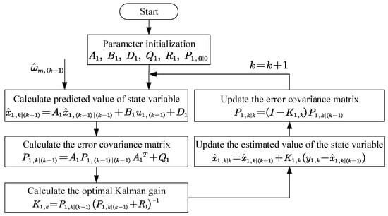
Figure 2.
The program flowchart of current observer.
According to the mechanical motion equation of the PMSM, one can define , . Disregarding the load as a time-varying disturbance, a second-order observer is constructed to observe the rotor angle and rotor angular velocity. Its state variable prediction equation is as follows:
here,
Then, (20) can be rewritten as the following:
The output state equation is as follows:
here, .
The implement flow chart of the position and speed observer based on the Kalman filter is shown in Figure 3.
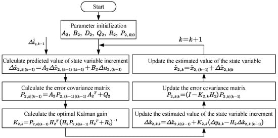
Figure 3.
The program flowchart of position and speed observer.
4.2. Improved Dual Second-Order Observer
The current observer designed in the previous section treats the speed as a constant value. To make the state estimation more accurate and realistic, disturbance observation is added. The coupling terms in the state equation are regarded as disturbances, so that the state variable prediction model of the second-order current observer is rewritten as the following:
In (23), is the state matrix only related to motor body parameters, which is a diagonal matrix; is the disturbance input matrix; is the disturbance variable. These are given by the following:
here, , and are the disturbance related to , , and , respectively.
Therefore, the disturbance observation model is established by the following:
In (24), , , and are the estimated disturbance values of the d-axis current disturbance, q-axis current disturbance, and mechanical angular velocity disturbance, respectively. , , and are the observer gains. , , and are the estimated values.
The discrete disturbance model in (24) is expressed by the following:
where is the disturbance gain matrix and is given by the following:
From (23), the optimized state space model is independent on the motor parameters. This is because some items related to the motor parameters are replaced by disturbance items, which reduces the sensitivity of the model to the motor parameters. This means that the improved state space model solves the model mismatch problem caused by the parameter disturbance and improves the robustness of the observer. The flow of the improved current observer based on the Kalman filter is shown in Figure 4.
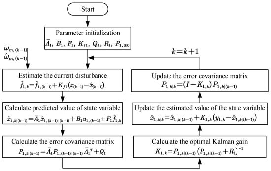
Figure 4.
The program flowchart of the improved current observer.
When establishing the position and speed observer (20) in the previous section, the load is regarded as a constant without considering its disturbance or change with time. Since the load disturbance will eventually cause a q-axis current disturbance, the q-axis current is used to estimate the load disturbance. Rewriting the motion state space model as the following:
here,
The disturbance state space model is given by the following:
here,
The flow of the improved position and speed observer based on the Kalman filter is shown in Figure 5.
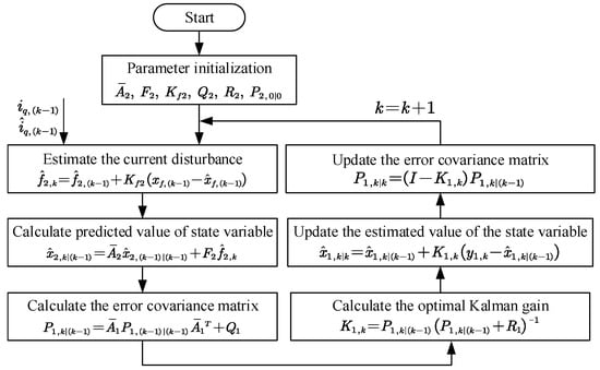
Figure 5.
The program flowchart of the improved position and speed observer.
5. Simulation Evaluation
To verify the effectiveness of the proposed observer, a simulation based on the MATLAB/simulink was carried out. The parameters of the PMSM are shown in Table 1. The switching frequency is set to 20 kHz. The reference mechanical speed is 1500 rpm, with a sudden load of 0.4 Nm at 0.15 s. To simulate the actual sampling situation, the noises to the current sampling data and position sampling data are added.

Table 1.
Parameters of the PMSM.
The estimation effect of the designed third-order observer (TO) on the state variables is verified. The comparison of the current of the d-axis and q-axis with the third-order observer and without any observer is shown in Figure 6, and the mechanical angular speed curve is shown in Figure 7. It can be seen from Figure 6 and Figure 7 that the ripple of the d-axis current, q-axis current, and speed are significantly reduced with the third-order observer. The simulation results show that the torque ripple can be effectively reduced when the third-order observer is used.
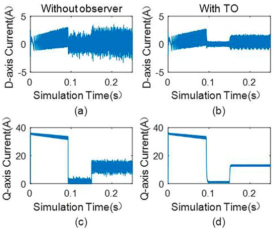
Figure 6.
(a) D−axis current without observer, (b) d−axis current with the third-order observer, (c) q−axis current without observer, and (d) q−axis current with the third-order observer.
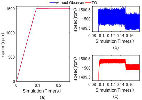
Figure 7.
(a) Global graph of the angular speed without observer and with the third-order observer, (b) local graph of the angular speed without observer, (c) local graph of the angular speed with the third-order observer.
The simulation results of the dual second-order observer (DSO) and third-order observer are shown in Figure 8 and Figure 9. From Figure 8 and Figure 9, the dual second-order observer shows a larger ripple of the d-axis current, q-axis current, and mechanical angular speed when the motor is at the steady state. This is because the use of the dual second-order observer cannot achieve complete decoupling of the state variables, resulting in a greater ripple in the estimated values of the state variables, and even greater errors between the estimated values and the actual values.
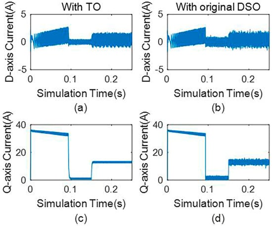
Figure 8.
(a) D−axis current with the third-order observer, (b) d−axis current with the original dual second-order observer, (c) q−axis current with the third−order observer, and (d) q−axis current with the original dual second−order observer.
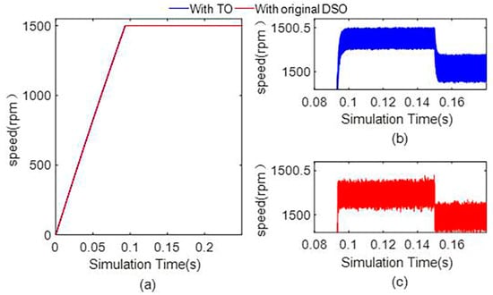
Figure 9.
(a) Global graph of the angular speed with the third−order observer and original second−order observer, (b) local graph of angular speed with the third−order observer, and (c) local graph of angular speed with the original second-order observer.
To solve the above problems, it is proposed to add the disturbance observation to the state prediction equation. This method can increase the estimation accuracy of each state and enhance the robustness of the state observer. Compared with the original dual second-order observer method, the comparison of the d-axis and q-axis current is shown in Figure 10, and the comparison of the motor mechanical speed curves is shown in Figure 11.
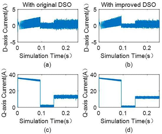
Figure 10.
(a) D−axis current with the original dual second−order observer, (b) d−axis current with the improved dual second−order observer, (c) q−axis current with the original dual second−order observer, and (d) q−axis current with the improved dual second−order observer.
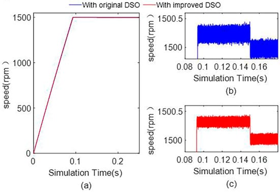
Figure 11.
(a) Global graph of the mechanical angular speed with the original dual second-order observer and improved dual second-order observer, (b) local graph of angular speed with the original dual second-order observer, and (c) local graph of angular speed with the improved dual second-order observer.
From Figure 10 and Figure 11, when the motor reaches the steady state, the current and speed pulsation of the d-axis and q-axis are reduced after adding the disturbance observation.
Low-speed operation with full loading is a challenge while dealing with Kalman filter-based observers. In this paper, low-speed operation with full loading is used to verify the superior performance of the original dual second-order observer and the improved dual second-order observer compared with that without the observer. The comparison of the motor mechanical speed, d-axis current, and q-axis current are shown in Figure 12, Figure 13 and Figure 14.
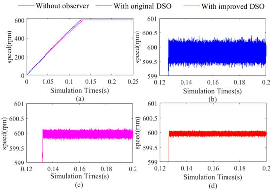
Figure 12.
(a) Global graph of the mechanical angular speed without observer, original dual second-order observer, and the improved dual second-order observer, (b) local graph of the angular speed without observer, (c) local graph of the angular speed with the original dual second-order observer, and (d) local graph of the angular speed with the improved dual second-order observer.
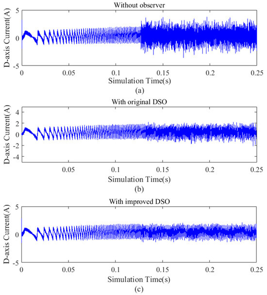
Figure 13.
(a) D−axis current without observer. (b) D−axis current with the original dual second− order observer. (c) D−axis current with the improved dual second−order observer.
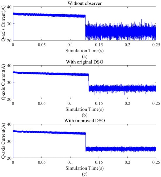
Figure 14.
Q−axis current comparison with different observers. (a) q−axis current without observer, (b) q−axis current with original dual second-order observer, and (c) q−axis current with the improved dual second−order observer.
It can be seen from Figure 12, Figure 13 and Figure 14 that under low-speed operation with full loading, the current and speed pulsation of axis D and Q of the improved dual second-order observer are better than the original dual second-order observer. This result also confirms the above conclusion.
To compare the estimation accuracy and evaluate the effectiveness of the third-order observer, original dual second-order observer, and the improved dual second-order observer, the average value and standard deviation (recorded as mean ± standard deviation) of the d-axis current, q-axis current, and rotor speed when the motor reaches steady state under no-load and load conditions are calculated, respectively. The mean value of the state variable is used to evaluate the estimation accuracy of the observer, and the standard deviation of the state variable is used to evaluate the ripple of the state variable. The more the mean value of the d-axis current tends to zero, the higher the estimation accuracy of d-axis current. The closer the q-axis current is to the average value of the q-axis current without any observer, the higher the estimation accuracy of the q-axis current is. The closer the mechanical angular velocity is to the reference value, the higher the estimation accuracy. The smaller the standard deviation, the smaller the ripple of the state variable. Under different working conditions, the calculation results of the state quantity estimation accuracy under each strategy are shown in Table 2, Table 3 and Table 4.

Table 2.
Estimation accuracy of state variable with different observers under no-load condition.

Table 3.
Estimation accuracy of state variable with different observers under 0.4 Nm load.

Table 4.
Estimation accuracy of state variable with different observers under 0.88 Nm load.
Under no-load condition, it can be seen from Table 2 that, the accuracy and precision of the state estimation are the highest with the third-order observer, and the average value of the state estimation is the closest to the real value. The mean error between the estimated value and the actual value of the d-axis current and q-axis current is 1.44% and 0.28%, respectively. And the estimated value has a small standard deviation difference, which is 0.1612 and 0.2707, respectively. While the standard deviation of the state estimation is small, the error between the estimated average value of the d-axis current, q-axis current, and the actual value is large; as high as 10.58% and 61.14%, respectively. When using the improved dual second-order observer with disturbance observation, the accuracy of the state estimation is significantly improved. The mean error between the estimated value and the actual value of the d-axis current and q-axis current is 3.85% and 0.00%, respectively. It is close to the state estimation accuracy of the third-order observer. And the standard deviation of the d-axis and q-axis current estimates are 0.2180 and 0.4442, respectively.
From Table 3, it can be concluded that under the 0.4 Nm load, using the third-order observer still has the best state estimation effect. The mean errors between the estimated and actual values of the d and q-axis currents are 4.21% and 0.0005%, respectively. Compared with the original dual second-order observer, the improved dual second-order observer shows better performance in both the accuracy and precision of the state estimation. The mean errors between the estimated and actual values of the d and q-axis currents are 6.18% and 0.0004%, respectively.
From Table 4, it can be concluded that under 0.88 Nm load, the improved dual second-order observer still has a better state estimation than the original dual second-order observer. The mean errors between the estimated and actual values of the d-axis currents are 3.56% and 4.19%, respectively. And the mean errors between the estimated and actual values of the q-axis currents are 0.0059% and 3.80%, respectively.
Comparing the data in Table 2, Table 3 and Table 4, it is not difficult to find that compared with the no-load condition, the current pulsation of the d-axis and q-axis are increased when the above-mentioned observers operate with 0.4 Nm and 0.88 Nm load. For the mechanical angular velocity, the estimation results using different observers are similar and very close to the real value. The reason for this is that compared with the current loop, the speed loop is the outer loop of the double closed-loop control system, and its output is only the given value of the q-axis current of the current loop. It does not directly drive the motor and has a relatively low running speed and stability.
The improved dual second-order observer has a great advantage: it is less sensitive to the model parameters. This means that when the motor is running, the influence of the motor parameter changes caused by temperature, humidity, and other environments on the state variable estimation is reduced, and it has strong robustness. To verify the robustness of the improved dual second-order observer, the inductance parameters of the motor are changed in the simulation, and the inductance value is set to half of the original value. The d-axis current, q-axis current, and mechanical angular velocity of the third-order observer and the dual second-order observer are compared. Figure 15 shows the current using the third-order observer and the improved dual second-order observer. Figure 16 shows the rotor speed curve using the third-order observer and the improved dual second-order observer. Table 5 and Table 6 show the calculation results of the state variable estimation accuracy when using a third-order observer and improved dual second-order observer under different load conditions.
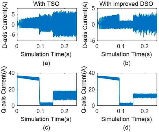
Figure 15.
Current with third−order observer and the proposed dual second−order observer in case of parameter mismatch. (a) D−axis current with third−order observer, (b) d−axis current with improved dual second−order observer, (c) q−axis current with the third−order observer, and (d) q−axis current with improved dual second−order observer.
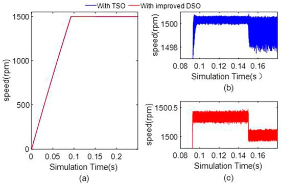
Figure 16.
Mechanical angular velocity with the third−order observer and proposed dual second− order observer in case of parameter mismatch. (a) Global graph of angular speed, (b) local graph of angular speed with the third−order observer, and (c) local graph of angular speed with the improved dual second−order observer.

Table 5.
Estimation accuracy of state variable using different methods under no-load condition.

Table 6.
Estimation accuracy of state variable using different methods under 0.4 Nm load.
It can be seen from Figure 15 and Figure 16, when the motor model parameters are mismatched, compared with using the improved dual second-order observer, using the third-order observer will produce a larger current and speed ripple. When the load is 0.4 Nm, the d-axis current and speed ripple increase sharply. However, the ripple of each state variable is relatively small when using the improved dual second-order observer. This phenomenon shows that the state variable estimation accuracy of the third-order observer depends on the accuracy of the model parameters. When the model is mismatched, the state estimation error is large, and even the system may vibrate. The improved dual second-order observer has more tolerance to the model parameters, and still has higher state estimation accuracy when the model is mismatched.
It can be seen from Table 5 and Table 6 that when the motor parameter model is mismatched, and the third-order observer is used to estimate the state variables, the average value and the standard deviation of the estimated current of the d-axis and q-axis differs greatly from the actual value. Under no-load and load conditions, the mean error between the estimated value of the d-axis current and the actual value is 120.07% and 70.16%, respectively. The mean error between the estimated value and the actual value of the q-axis current is 55.20% and 6.52%, respectively. When using the improved dual second-order observer, the mean error between the estimated value and the actual value of the d-axis current is 35.16% and 19.82%, respectively under no-load and load conditions. The mean error between the estimated value of the q-axis current and the actual value is 0.16% and 0.03%, respectively. For the rotor speed estimation, both observers have high accuracy, that is, the mean error between the estimated value and the actual value is very small, both less than 0.03%. When the third-order observer is used in the load operation, the inaccuracy of the motor parameters will lead to a greater speed ripple, that is, there is a relatively large standard deviation in the speed estimation value, which is 0.0687; much greater than 0.0153 in no-load operation. When using the improved dual second-order observer, the standard deviation of the speed estimation both under no-load and load operation is about 0.0030.
6. Experiment Evaluation
The main body of the test bench in Figure 17 is composed of modules, dynamic torque sensors, magnetic powder brakes, and two couplings. The output of the module is connected to the input of the torque sensor through the output flange and coupling, and the output of the torque sensor is connected to the input of the magnetic particle brake through the coupling. The module is highly integrated by a surface mounted permanent magnet synchronous motor, motor drive control board, and planetary reducer. The reduction ratio of the planetary reducer is 1:9.1. The measuring range of the dynamic torque sensor is 0–50 Nm. The function of the magnetic powder brake is to simulate the load. By changing the input current, the output torque can be changed linearly to provide different loads.
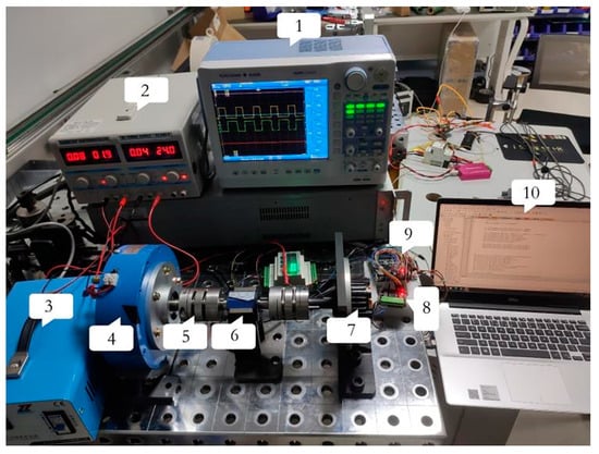
Figure 17.
System prototype. (1) Oscillograph, (2) digital power supply, (3) isolated power supply, (4) magnetic powder brake, (5) coupler, (6) dynamic torque sensor, (7) module (including motor, control board and planetary reducer), (8) AD conversion module, (9) data acquisition board, and (10) computer.
To further verify the effectiveness of the proposed observer, comparative experiments were carried out under no-load and load conditions without the observer, with a dual second-order observer and improved dual second-order observer.
The motor operates at the no-load condition and the given reference mechanical angular speed is 1500 rpm. The experimental results with the different observer strategies are shown in Figure 18, Figure 19 and Figure 20. Figure 18 shows the d-axis current under different observer strategies. Figure 19 shows the q-axis current under different observer strategies, and Figure 20 shows the rotor speed response curve under different observer strategies. Table 7 shows the current and speed estimation accuracy with different observer strategies under no-load conditions.
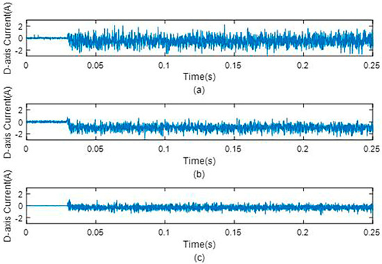
Figure 18.
D−axis current under different observers under no−load condition. (a) D−axis current without observer, (b) that with the original dual second−order observer, and (c) that with the improved dual second−order observer.
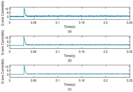
Figure 19.
Q−axis current under different observers under no−load condition. (a) Q−axis current without observer, (b) q−axis current with the original dual second−order observer, and (c) q−axis current with the proposed dual second−order observer.
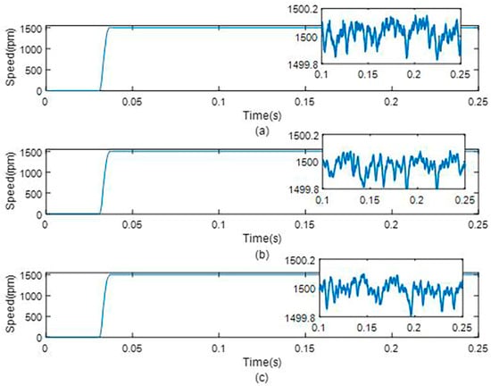
Figure 20.
Mechanical angular speed response under different observers under no−load condition. (a) Speed without observer. (b) That with the original dual second−order observer, and (c) that with the proposed dual second−order observer.

Table 7.
State estimation accuracy with different observer strategies under no-load condition.
From Figure 18, Figure 19 and Figure 20, the current ripple of the d-axis and q-axis in the steady state is significantly reduced when using the dual second-order observer. There is no obvious difference in the mechanical angular velocity, and the speed ripple is small. The improved observer is better than the original observer in the estimation of the current. Using the improved state observer can reduce the current ripple of the d-axis and q-axis, and enhance the anti-interference ability of current loop.
From the data in Table 7, when using the unimproved dual second-order observer, the errors between the average value of the d-axis current and q-axis current and those without observer are 61.42% and 52.70%. The inaccuracy of the d-axis current and q-axis current estimation are caused by the inaccuracy of the motor model and disturbances in the system. When using the improved dual second-order observer strategy, the estimation accuracy of the d-axis current and q-axis current are significantly improved, and the ripple is smaller in the steady state. Compared with no observer, the d-axis current standard deviation is reduced by 33.67% and 52.23%, respectively, and the q-axis current standard deviation is reduced by 42.22% and 59.99%, respectively by using the original dual second-order observer and the improved dual second-order observer. When using different observer strategies, the motor speed estimates are all close to the speed reference with less ripple. Compared with no observer, when using the original and improved dual second-order observer, the mechanical angular velocity standard deviation is reduced by 15.75% and 21.61%, respectively. The performance of the improved observer in terms of mechanical angular velocity estimation is only slightly improved compared to before the improvement. This is because the speed loop belongs to the outer loop of the control system. Compared with the inner loop, the operating frequency is slower, and it has higher anti-interference performance than the current loop.
To verify the effectiveness of the proposed observer under load conditions, and to compare the performance of the improved dual second-order observer, comparative experiments are carried out without any observer, with original dual second-order observer and with improved dual second-order observer under the load of 0.25 Nm and 0.8 Nm. And the speed reference value is 1500 rpm and 600 rpm, respectively. Figure 21, Figure 22, Figure 23, Figure 24, Figure 25 and Figure 26 show the steady-state curves of the d-axis current, q-axis current, and mechanical angular velocity under different observer strategies. Table 8 and Table 9 shows the estimation accuracy of each state variable under different observer strategies.
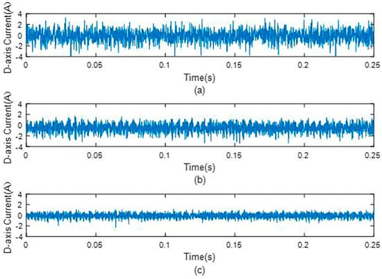
Figure 21.
D−axis current under different observers under 0.25 Nm load condition. (a) D−axis current without observer, (b) that with the original dual second−order observer, and (c) that with the improved dual second−order observer.
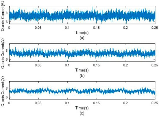
Figure 22.
Q−axis current under different observers under 0.25 Nm load condition. (a) Q−axis current without observer, (b) q−axis current with the original dual second−order observer, and (c) q−axis current with the improved dual second−order observer.
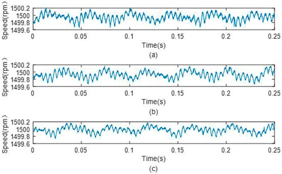
Figure 23.
Mechanical angular speed with different observers under 0.25 Nm load condition. (a) Angular speed without observer, (b) that with the original dual second−order observer, and (c) that with the improved dual second−order observer.
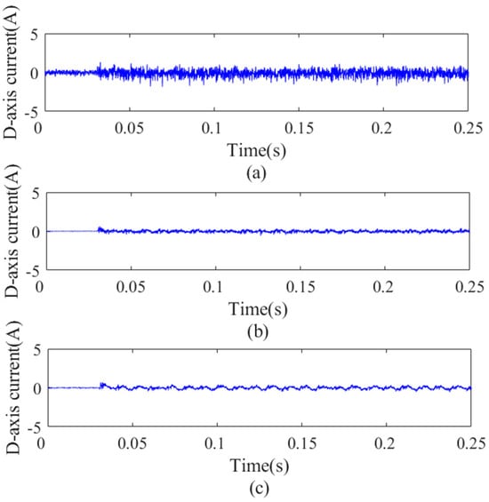
Figure 24.
D−axis current under different observers under 0.8 Nm load condition. (a) D−axis current without observer, (b) that with original dual second−order observer, and (c) that with improved dual second−order observer.
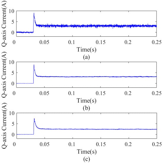
Figure 25.
Q−axis current under different observers under 0.8 Nm load condition. (a) Q−axis current without observer, (b) that with the original dual second−order observer, and (c) that with the improved dual second−order observer.
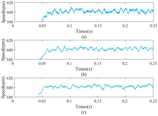
Figure 26.
Mechanical angular speed with different observers under 0.8 Nm load condition. (a) Angular speed without observer, (b) that with original dual second−order observer, and (c) that with improved dual second−order observer.

Table 8.
State estimation accuracy with different observer strategies under 0.25 Nm load condition.

Table 9.
State estimation accuracy with different observer strategies under 0.8 Nm load condition.
It can be seen from Figure 21, Figure 22, Figure 23 and Figure 24 that compared with no-load condition, the current ripple in the steady state is increased under the load condition. Compared with the case without the observer, the steady-state current and current ripple is significantly reduced by using the dual second-order observer. It can be seen from Figure 23 and Figure 26 that compared with the no-load condition, the motor rotor speed ripple increases under the load condition, and the error with the reference value slightly increases. It shows that the steady-state performance of the motor decreases under load conditions.
By analyzing the data in Table 8, after using the dual second-order observer, the current standard deviation of the d-axis and q-axis decreases in the steady state. Compared with the case without an observer, when using the original and improved dual second-order observer, the d-axis current standard deviation is reduced by 19.90% and 56.08%, respectively, and the q-axis current standard deviation is reduced by 36.80% and 55.50%, respectively. Especially when using the improved dual second-order observer, the estimated value of the state variable is closer to the actual value and has higher estimation accuracy. Compared with no observer, when using the original and improved dual second-order observer, the mechanical angular velocity standard deviation is reduced by 3.56% and 12.37%, respectively.
By analyzing the data in Table 9, it also can be seen that after using the dual second-order observer, the current standard deviation of the d-axis and q-axis decreases in the steady state. Compared with the case without any observer, when using the original and improved dual second-order observer, the d-axis current standard deviation is reduced by 68.80% and 63.76%, respectively and the q-axis current standard deviation is reduced by 70.90% and 73.09%, respectively. Compared with no observer, when using the original and improved dual second-order observer, the mechanical angular velocity standard deviation is reduced by 14.15% and 43.20%, respectively.
In a word, the experimental results show that the proposed dual second-order observer is effective and accurate in the estimation of the d-axis current, q-axis current, and rotor speed. The current ripple of the motor is significantly reduced. And it is more accurate in the estimation of the state variables. Also, it can reduce the torque ripple and improve the steady-state performance of the system.
7. Conclusions
The third-order observer is an effective solution to estimate simultaneously the d-axis current, q-axis current, and speed of the PMSM with low noise and high stability. To reduce its dependence on the model and the computational burden, and also improve its robustness, the authors propose an improved dual second-order observer based on the Kalman filter with a disturbance observation added. A simulation platform and experimental prototype are demonstrated to verify the analysis. From the simulation and experimental results, one can get the following conclusions:
- The estimation accuracy of the speed of the TO and improved DSO is 1500.0396 ± 0.0090 and 1500.0320 ± 0.0030 under a 0.4 Nm load, respectively. And the ripple of the current of the iq of the improved DSO is 4.64%. The simulation results show that the proposed dual second-order observer can approach the estimation accuracy with the third-order observer and has a relatively small ripple of current and mechanical angular velocity.
- The estimation accuracy of the speed of the improved DSO is 1499.9780 ± 0.0836 under a 0.25 Nm load, and the ripple of the current iq is 3.87%. The experimental results show that the proposed observer can realize a higher precision estimation of the state variables and can effectively suppress the current and mechanical angular velocity ripple.
- When the motor model parameters are mismatched, the estimation accuracy of the iq of the TO and improved DSO is 13.0677 ± 2.3381 and 12.2653 ± 1.0047 under a 0.4 Nm load, respectively. Compared with the third-order observer and the original dual second-order observer, the proposed dual second-order observer in this paper has better robustness in terms of the estimation of the state variables. It also has a higher tolerance to the uncertainty of the motor model and system interference.
Author Contributions
Conceptualization, G.Z.; methodology, Y.Z.; software, X.D.; validation, Y.Z., X.D. and J.L.; writing—original draft preparation, Y.Z.; writing—review and editing, J.L. All authors have read and agreed to the published version of the manuscript.
Funding
This research received no external funding.
Data Availability Statement
Not applicable.
Conflicts of Interest
The authors declare no conflict of interest.
References
- Chenwei, Y.; Fei, D.; Yi, A.; Fengqing, Z. Design and analysis of permanent magnet synchronous servo motor with low rotational inertia and high torque density. J. Phys. Conf. Ser. 2021, 1965, 012010. [Google Scholar] [CrossRef]
- Wensing, P.M.; Wang, A.; Seok, S.; Otten, D.; Lang, J.; Kim, S. Proprioceptive Actuator Design in the MIT Cheetah: Impact Mitigation and High-Bandwidth Physical Interaction for Dynamic Legged Robots. IEEE Trans. Robot. 2017, 33, 509–522. [Google Scholar] [CrossRef]
- Kenneally, G.; De, A.; Koditschek, D.E. Design Principles for a Family of Direct-Drive Legged Robots. IEEE Robot. Autom. Lett. 2016, 1, 900–907. [Google Scholar] [CrossRef]
- Le, D.P.; Choi, J.; Kang, S. External force estimation using joint torque sensors and its application to impedance control of a robot manipulator. In Proceedings of the 2013 13th International Conference on Control, Automation and Systems (ICCAS 2013), Gwangju, Republic of Korea, 20–23 October 2013; pp. 1794–1798. [Google Scholar] [CrossRef]
- Cong, Z.; Chuang, L.; Kai, W. A novel single resistance current sampling technique of switched reluctance motor. Trans. China Electrotech. Soc. 2017, 32, 55–61. [Google Scholar]
- Kanungo, A.; Mittal, M.; Dewan, L.; Mittal, V.; Gupta, V. Speed control of DC motor with MRPID controller in the presence of noise. Wirel. Pers. Commun. 2022, 124, 893–907. [Google Scholar] [CrossRef]
- Liu, X.; Wang, Z.; Wang, W.; Lv, Y.; Yuan, B.; Wang, S.; Li, W.; Li, Q.; Zhang, Q.; Chen, Q. SMO-based sensorless control of a permanent magnet synchronous motor. Front. Energy Res. 2022, 10, 839329. [Google Scholar] [CrossRef]
- Pal, D. Modeling, analysis and design of a DC motor based on state space approach. Int. J. Eng. Res. 2016, 5, 293–296. [Google Scholar] [CrossRef]
- Hinkkanen, M.; Saarakkala, S.E.; Awan, H.A.A.; Molsa, E.; Tuovinen, T. Observers for Sensorless Synchronous Motor Drives: Framework for Design and Analysis. IEEE Trans. Ind. Appl. 2018, 54, 6090–6100. [Google Scholar] [CrossRef]
- Luenberger, D.G. Observing the State of a Linear System. IEEE Trans. Mil. Electron. 1964, 8, 74–80. [Google Scholar] [CrossRef]
- Horch, M.; Boumédiène, A.; Baghli, L. Sensorless high-order sliding modes vector control for induction motor drive with a new adaptive speed observer using super-twisting strategy. Int. J. Comput. Appl. Technol. 2019, 59, 144–153. [Google Scholar] [CrossRef]
- Zhou, M.; Cheng, S.; Feng, Y.; Xu, W.; Wang, L.; Cai, W. Full-Order Terminal Sliding-Mode-Based Sensorless Control of Induction Motor with Gain Adaptation. IEEE J. Emerg. Sel. Top. Power Electron. 2022, 10, 1978–1991. [Google Scholar] [CrossRef]
- Ren, X.; Li, D.; Sun, G.; Zhao, W. Eso-based adaptive robust control of dual motor driving servo system. Asian J. Control. 2016, 18, 2358–2365. [Google Scholar] [CrossRef]
- Su, J.; Chen, W.-H.; Yang, J. On relationship between time-domain and frequency-domain disturbance observers and its applications. J. Dyn. Syst. Meas. Control. 2016, 138, 091013. [Google Scholar] [CrossRef]
- Zhang, X.; Sun, L.; Zhao, K.; Sun, L. Nonlinear Speed Control for PMSM System Using Sliding-Mode Control and Disturbance Compensation Techniques. IEEE Trans. Power Electron. 2013, 28, 1358–1365. [Google Scholar] [CrossRef]
- Yan, Y.; Yang, J.; Sun, Z.; Zhang, C.; Li, S.; Yu, H. Robust Speed Regulation for PMSM Servo System with Multiple Sources of Disturbances via an Augmented Disturbance Observer. IEEE/ASME Trans. Mechatron. 2018, 23, 769–780. [Google Scholar] [CrossRef]
- Zhao, Y.; Dong, L. Robust current and speed control of a permanent magnet synchronous motor using SMC and ADRC. Control Theory Technol. 2019, 17, 190–199. [Google Scholar] [CrossRef]
- Du, B.; Wu, S.; Han, S.; Cui, S. Application of Linear Active Disturbance Rejection Controller for Sensorless Control of Internal Permanent-Magnet Synchronous Motor. IEEE Trans. Ind. Electron. 2016, 63, 3019–3027. [Google Scholar] [CrossRef]
- Qu, L.; Qiao, W.; Qu, L. Active-Disturbance-Rejection-Based Sliding-Mode Current Control for Permanent-Magnet Synchronous Motors. IEEE Trans. Power Electron. 2021, 36, 751–760. [Google Scholar] [CrossRef]
- Liu, X.; Yu, H.; Yu, J.; Zhao, L. Combined Speed and Current Terminal Sliding Mode Control With Nonlinear Disturbance Observer for PMSM Drive. IEEE Access 2018, 6, 29594–29601. [Google Scholar] [CrossRef]
- Yi, Y.; Sun, X.; Li, X.; Fan, X. Disturbance observer based composite speed controller design for PMSM system with mismatched disturbances. Trans. Inst. Meas. Control. 2016, 38, 742–750. [Google Scholar] [CrossRef]
- Wang, Y.; Yu, H.; Liu, Y. Speed-Current Single-Loop Control with Overcurrent Protection for PMSM Based on Time-Varying Nonlinear Disturbance Observer. IEEE Trans. Ind. Electron. 2022, 69, 179–189. [Google Scholar] [CrossRef]
- Akram, M.A.; Liu, P.; Tahir, M.O.; Ali, W.; Wang, Y. A state optimization model based on Kalman filtering and robust estimation theory for fusion of multi-source information in highly non-linear systems. Sensors 2019, 19, 1687. [Google Scholar] [CrossRef] [PubMed]
- Lund, S.H.J.; Billeschou, P.; Larsen, L.B. High-bandwidth active impedance control of the proprioceptive actuator design in dynamic compliant robotics. Actuators 2019, 8, 71. [Google Scholar] [CrossRef]
- Nair, D.S.; Jagadanand, G.; George, S. Torque estimation using kalman filter and extended Kalman filter algorithms for a sensorless direct torque controlled BLDC motor drive: A comparative study. J. Electr. Eng. Technol. 2021, 16, 2621–2634. [Google Scholar] [CrossRef]
- Yang, R.; Li, L.-Y.; Wang, M.-Y.; Zhang, C.-M.; Zeng-Gu, Y.-M. Force Ripple Estimation and Compensation of PMLSM With Incremental Extended State Modeling-Based Kalman Filter: A Practical Tuning Method. IEEE Access 2019, 7, 108331–108342. [Google Scholar] [CrossRef]
Disclaimer/Publisher’s Note: The statements, opinions and data contained in all publications are solely those of the individual author(s) and contributor(s) and not of MDPI and/or the editor(s). MDPI and/or the editor(s) disclaim responsibility for any injury to people or property resulting from any ideas, methods, instructions or products referred to in the content. |
© 2023 by the authors. Licensee MDPI, Basel, Switzerland. This article is an open access article distributed under the terms and conditions of the Creative Commons Attribution (CC BY) license (https://creativecommons.org/licenses/by/4.0/).