MEVO: A Metamodel-Based Evolutionary Optimizer for Building Energy Optimization

Abstract

A deep energy retrofit of building envelopes is a vital strategy to reduce final energy use in existing buildings towards their net-zero emissions performance. Building energy modeling is a reliable technique that provides a pathway to analyze and optimize various energy-efficient building envelope measures. However, conventional optimization analyses are time-consuming and computationally expensive, especially for complex buildings and many optimization parameters. Therefore, this paper proposed a novel optimization algorithm, MEVO (metamodel-based evolutionary optimizer), developed to efficiently identify optimal retrofit solutions for building envelopes while minimizing the need for extensive simulations. The key innovation of MEVO lies in its integration of evolutionary techniques with design-of-computer experiments, machine learning, and metaheuristic optimization. This approach continuously refined a machine learning model through metaheuristic optimization, crossover, and mutation operations. Comparative assessments were conducted against four alternative metaheuristic algorithms and Bayesian optimization, demonstrating MEVO’s effectiveness in reliably finding the best solution within a reduced computation time. A hypothesis test revealed that the proposed algorithm is significantly better than Bayesian optimization in finding the best cost values. Regarding computation time, the proposed algorithm is 4–7 times faster than the particle swarm optimization algorithm and has a similar computational speed as Bayesian Optimization.

1. Introduction

Building energy use corresponds to 30% of the world’s energy consumption [1]. Specifically, buildings’ electricity consumption accounts for roughly 55% of global electricity consumption [2], while natural gas in residential, commercial, and public sectors accounts for 48% of global natural gas consumption [3]. The International Energy Agency has suggested that deep energy retrofitting of building envelopes is a vital strategy to reduce final energy use in buildings towards a net-zero emission goal by 2070 [2]. Building performance simulation (BPS) (typically, a building performance simulator predicts the energy use per unit of time, given weather information, a building geometry, an HVAC description, and a utility rate structure) is a reliable method that offers the opportunity to assess, evaluate, and enhance different energy-efficient building envelope strategies and technologies. Therefore, BPSs can support the development of more informed design solutions and facilitate compliance with energy regulations and guidelines.

Building performance optimization (BPO) aims at finding the optimal solution from a set of feasible solutions for a given design or retrofitting problem [4]. The optimal solution is determined based on specific performance criteria called objective functions. In the context of BPO, these objective functions could include minimizing costs, reducing energy consumption, or increasing occupants’ comfort. Finding the optimal solution through direct optimization usually involves hundreds or thousands of objective function evaluations, resulting in time-consuming processes when utilizing BPS tools and optimization algorithms.

This problem can be addressed by employing approaches, such as multi-stage optimization algorithms [5,6] or parallel computing [7,8], which enhance the computational capabilities of traditional simulation-based optimization methods. However, even multi-stage optimization algorithms and parallel computing require many simulations to guarantee convergence. Consequently, applying the simulation-based approaches to scenarios is impractical due to computational burden.

To tackle this issue, “surrogate models” can be used instead of traditional simulation-based optimization methods. Surrogate models are created using simulation data, approximating the original model. There are two main categories of surrogate models: static surrogate models [9,10,11,12,13], trained using an initial set of sampling points, and iterative surrogate models [14,15,16,17,18], that gradually add samples during optimization. The accuracy of static surrogate models is limited via the initial precision of the trained model, while iterative models increase their accuracy during optimization. The current study proposed a novel optimization algorithm based on an iterative surrogate model that decreases the required computational burden by reducing the number of required simulations, thereby allowing enhanced assessment of energy retrofit projects by expeditiously exploring a wider domain of scenarios.

1.1. Literature Review

In response to the time-consuming optimization process, scholars have proposed various approaches to reduce the computation burden while maintaining acceptable levels of accuracy. One proposed approach involves tackling the BPO problem through a multi-stage process to reduce complexity. The multi-stage approach entails conducting the optimization process in several stages, each involving lighter computations rather than a single step with heavy computations. However, it is worth noting that due to the separation of certain BPS and decision variables in the optimization stages, there is a possibility that the overall integrity of the process might be somewhat compromised. Ascione et al. [5] proposed a three-objective and multi-stage GA optimization framework to minimize CO₂ emissions, energy consumption and global cost of a typical newly built Italian office building. In the first stage, envelope, HVAC operation, and geometry variables are optimized using the GA algorithm. Next, an exhaustive sampling is performed in the second stage on the optimal solution resulting from the first stage to find optimal energy systems. Finally, the third stage recommends design solutions based on sustainability, cost optimality, and investment cost criteria under different budget constraints. Ciardiello et al. [6] developed a multi-objective and multi-stage NSGA-II optimization framework to optimize the energy performance of a newly built residential building in the Mediterranean climate. In the first stage, geometry characteristics, including shape, shape proportion, window-to-wall ratio, and orientation, are optimized to minimize heating, cooling, and total energy demand. Subsequently, in the second stage, passive and active strategy optimization is performed on the optimal solution obtained from the first stage. In detail, total energy demand, annual energy cost, investment cost, and CO₂ emissions are minimized by optimizing envelope, morphology, renewable energy systems, photovoltaic systems, and solar thermal systems.

Another approach to reducing computational time is utilizing a parallel computing approach. This method divides a complex and time-consuming problem into smaller subtasks, distributed among multiple workers and executed simultaneously and independently. The results from each worker are then combined to obtain the outcome. The parallel algorithm structure leverages the capabilities of multi-core processors to conduct calculations much faster, which proves crucial for handling data-intensive simulation-based optimization processes [7,8]. In their study, Mostafazadeh et al. [7] presented a simulation-based framework to optimize the environmental, economic, and social aspects of building energy retrofits, while considering climate change and energy price variations on a residential building in Iran. A modified version of NSGA-III called prNSGA-III was developed by incorporating a parallel computing structure that enables simultaneous simulations using multi-core processors and a result-saving archive to avoid redundant computations and alleviate the computational workload, significantly reducing its processing time.

Although the existing literature [5,6,7,8,19,20] indicates that simulation-based optimization algorithms offer improved efficiency when compared to exhaustive search methods, it is essential to note that these algorithms still require a significant amount of time due to the necessity of exploring a large number of options to achieve convergence. The total optimization time remains considerable, even with methods like multi-stage optimization or parallel computing. Consequently, applying these simulation-based approaches to various building categories becomes challenging when dealing with complex case studies and scenarios due to the significant computational burden. In this regard, surrogate models, also called metamodels, can reduce the computational burden of optimization procedures [21].

Surrogate models are created using simulation data, enabling them to approximate the original model and enhance optimization algorithms’ efficiency. The most commonly employed techniques for building surrogate models include statistical methods, like polynomial regression, as well as machine learning methods, such as artificial neural networks (ANNs), support vector regression (SVR), Gaussian process regression (also known as Kriging), random forest, and gradient boosting [22]. In the conventional method, surrogate models are constructed using a static approach [23]. This approach involves generating a sampling plan, conducting simulations based on this plan, and then fitting the surrogate model with the obtained simulation data. Subsequently, the optimization process utilizes the constructed surrogate model rather than conducting simulations during the optimization phase, leading to significant time savings. Several studies have investigated the application of static approaches.

Melo et al. [9] employed the Latin hypercube sampling (LHS) method to generate a vast dataset of 1 million samples. These samples were subsequently simulated using parallel computing to compare the performance of surrogates built with various techniques, including multiple linear regression (MLR), artificial neural networks (ANNs), multivariate adaptive regression splines (MARS), support vector regression (SVR), random forests (RFs), and Gaussian process (GP). These researchers found that ANN surrogate models outperformed the other techniques in predicting cooling energy demand and exhibited faster training times.

Sharif et al. [10] developed an artificial neural network (ANN) as a surrogate model in their research. They utilized data derived from the simulation-based multi-objective optimization (SBMO) model. Their research highlighted the effectiveness of the ANN model in predicting total energy consumption (TEC), life cycle cost (LCC), and life cycle assessment (LCA) across different building renovation scenarios. These scenarios encompassed several factors, such as the building envelope, HVAC system, and lighting systems. Nevertheless, to enhance the accuracy of their predictions, it was found that increasing the number of initial simulations was necessary, which, in turn, resulted in longer computational times. Razmi et al. [11] investigated an optimal dormitory building early stage design to enhance energy efficiency, daylight, and thermal comfort using a PCA-ANN-integrated NSGA-III. They used 2000 sampling points from the LHS method to train their ANN model. For generating initial sampling points, Chegari et al. [12] used a mathematical approach to determine the minimum number of simulations required for maximum accuracy in generating a surrogate model. They combined an ANN surrogate model with MOPSO to optimize annual thermal energy demand and the annual weighted average of discomfort degree hours of a typical Moroccan building in several climate zones. Kubwimana et al. [13] introduced a novel method for optimizing building energy performance through Python and EnergyPlus. An artificial neural network was employed to construct a static surrogate model, which was optimized using Bayesian optimization and a genetic algorithm. This approach was assessed through a case study involving an eight-parameter exploration for a building at the Florida Institute of Technology in Melbourne, FL, USA. The results illustrated faster convergence through Bayesian optimization compared to the GA.

While surrogate models increase the speed of the optimization process, their accuracy is limited by the initial precision of the trained model. An increased number of initial points for higher accuracy would translate into a higher computational burden, rendering this approach’s speed advantage ineffective [24]. An alternative surrogate modeling approach is the iterative approach [23], which involves gradually adding samples during optimization. Initially, a set of samples is required to build the surrogate model, but subsequently, the model is updated with each iteration of the optimization process upon incorporating a new sample. In this iterative approach, the new sample selection is determined by maximizing or minimizing an acquisition function, also called an infill sampling criterion, using an optimization algorithm at each iteration. Iterative approaches can achieve higher accuracy with fewer simulations [23,24].

Gengembre et al. [14] presented an iterative approach to minimize building energy consumption based on efficient global optimization (EGO). This method maximizes a modified and expected improvement function for selecting the new sampling points [25]. The surrogate model was constructed using Gaussian process regression, and optimization of the acquisition function was conducted through the particle swarm optimization (PSO) algorithm, with 1000 iterations and 50 particles. A maximum limit of 150 simulations was imposed, considering penalization functions related to investment costs and real continuous decision variables [14].

Tresidder et al. [15] adopted a Kriging model optimization approach to minimize CO₂ emissions and material costs. They iteratively updated the Kriging model by maximizing the expected improvement function with 60 initial samples obtained with the LHS method and 140 additional ones using the iterative approach. To assess their approach’s performance, they employed a two-tailed t-test, averaging the values from 10 runs for both the solution and objective functions. Furthermore, they compared the convergence of their model with a genetic algorithm (GA), demonstrating that the Kriging model optimization approach converges to the optimum solution more rapidly.

Gilan et al. [16] introduced an iterative learning scheme to tackle a multi-objective optimization problem in their study. They integrated NSGA-II with the Gaussian process (GP) to prioritize the simulation of solutions that are highly informative for the model’s predictions during each generation, in addition to the initial ones generated using the LHS method. The model optimized the heating and cooling energy consumption rates of an archetype office building in the UK. The outcomes revealed that the iterative learning approach outperformed both static and simulation-based methods.

Bamdad et al. [17] introduced a novel iterative learning surrogate model, denoted L-SOAS, to optimize building energy performance. The model uses parameter spaces with lower energy use and higher uncertainty for new sampling point selection. L-SOAS was compared to optimization based on a surrogate model with random sampling and simulation-based optimization methods. L-SOAS achieved better optimization results with a lower number of simulations.

Lahmar et al. [18] presented an efficient multi-objective optimization approach called AKSUMO, which utilizes Kriging surrogate models to optimize building designs. The surrogate model replaces time-intensive simulations with approximations, employing an adaptive sampling algorithm to enhance accuracy in the vicinity of Pareto solutions. A Latin hypercube design (LHD) was used to generate 40 sampling points to initiate the learning process of the surrogate model. The framework was applied to a Moroccan residential building to optimize the investment and energy consumption costs. The AKSUMO method significantly reduced the number of building simulations by up to 50%.

1.2. Research Gap and Contribution

The literature review highlights the need to further improve the computational speed and efficiency of the previous frameworks for enhancing building performance. In this respect, reducing the required computational time makes exploring multiple scenarios with a broad range of possibilities and situations feasible. While surrogate-based models offer enhancements compared to simulation-based optimization strategies, employing pre-trained neural networks as predictive models demands extensive training data to ensure precise predictions across design variables. Additionally, methods relying on a static surrogate model that remains unchanged throughout the optimization process may encounter challenges in predictive efficacy, as the exploration uncovers configurations that significantly deviate from the training dataset.

The computational shortcomings highlighted above are pervasive in various large-scale, expensive black-box optimization problems. This study proposed a novel method to achieve a more cohesive integration of the machine learning and optimization components. This method is a specific variant of incremental learning intended to enhance the surrogate model throughout an evolutionary optimization process. The proposed predictive model was trained using a limited set of simulated samples to realize computational efficiency. Nonetheless, as the optimization proceeds, extra configurations are simulated and subsequently incorporated into the training data. As a result, the metamodel self-updates through the iterative process of the sampling points generation, thereby enhancing its predictive accuracy. In this study, an artificial neural network model was used for prediction, and a novel and fast version of PSO, named MEPSO, was used to optimize the acquisition function. Compared to PSO, MEPSO showcases reduced computational complexity and a faster convergence rate [26].

Our active learning strategy utilized a novel approach for selecting new sampling points through three distinct approaches: the optimal result of the MEPSO algorithm, crossover, and mutation at each generation. Applying these three strategies, which include the iterative surrogate model, the MEPSO optimization algorithm, and the utilization of crossover and mutation in the selection of new sampling points, can decrease the optimization time and enhance the convergence of the optimal solution set.

In addition, the capability of the developed framework was investigated using an actual commercial building characterized by widespread construction technologies in Canadian building stock. Therefore, the results can provide informative insights for building industry associates in the public and private sectors. Previous research has explored various methodologies to accelerate optimization (as previously cited). However, no comprehensive design approach has put forth an all-inclusive study of the following aspects:

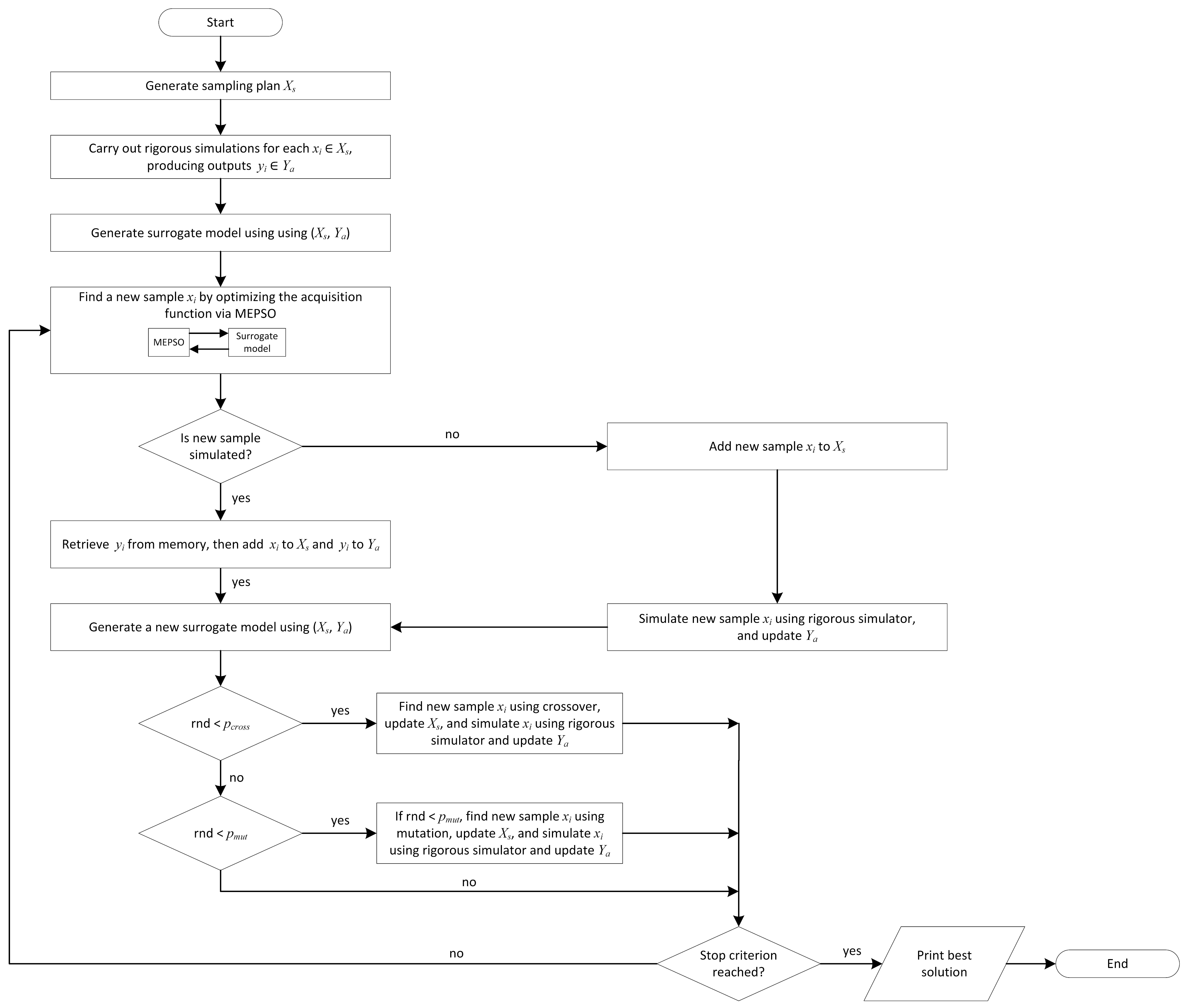
• The proposed novel method integrates machine learning and optimization via active learning, enhancing the surrogate model within evolutionary optimization by training on limited simulated samples and incorporating additional configurations for a self-updating metamodel, resulting in improved predictive accuracy.
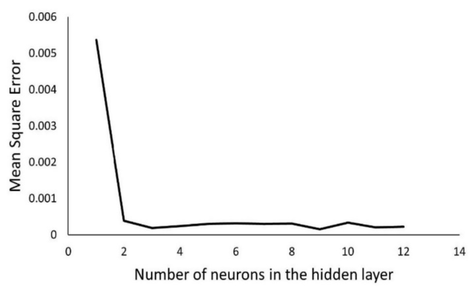
• Utilization of an artificial neural network for prediction and a faster version of particle swarm optimization (MEPSO) for optimization, demonstrating reduced complexity and faster convergence compared to conventional PSO.
• An active learning strategy selects three distinct approaches for simulating offspring at each new generation, involving the optimal MEPSO outcome, crossover, and mutation, aiming to decrease optimization time and enhance convergence of the optimal solution set.
• Application of the developed framework on an actual commercial building with widespread Canadian construction technologies, offering valuable insights for building industry stakeholders in both the public and private sectors.

This paper contributes to the existing literature by developing an efficient algorithm to analyze energy retrofit projects, specifically for Canadian commercial building stock. The workflow of the MEVO algorithm has been detailed in the following section.

2. Methodology

This paper presents a novel metamodel-based evolutionary optimization (MEVO) for finding optimal building retrofit solutions. This surrogate model-based optimization algorithm was implemented in Python and coupled to EnergyPlus, which was used as a building performance simulator. SketchUp was used as the graphical user interface of EnergyPlus for developing the geometry of the building model. These programs hold reputable accreditations and are widely utilized within commercial and academic circles. EnergyPlus is a widely used and reliable BPS tool that uses text-based input/output (ASCII) files, enabling easy alteration of input data files (.IDF) and processing output files (.CSV). Python was used as a console tool for handling EnergyPlus input/output files, post-processing the data, implementing optimization processes, and generating and updating surrogate models. Python is highly regarded for its proficiency in handling text file processing tasks. Additionally, it offers reliable support and exceptional capabilities in data processing, machine learning, and statistical analysis. The performance of the newly developed optimization framework was examined through a comparative analysis with well-established algorithms in the domain of building energy optimization, namely particle swarm optimization (PSO) and genetic algorithm (GA). Furthermore, it was compared with micro evolutionary particle swarm optimization (MEPSO), a new metaheuristic optimization algorithm [22], and an integral component of the metamodel-based evolutionary optimization (MEVO) framework. Lastly, MEVO was compared with Bayesian optimization due to its structural similarities. The proposed methodology consists of the five following steps:

• Defining the case building and calibrating the generated model.
• Incorporating the retrofit options and generating a parametric model.
• Formulating the objective function.
• Implementing the optimization strategy (MEVO).
• Evaluating the performance of MEVO optimization by comparing it to MEPSO, PSO, GA, and Bayesian optimizations.

The proposed methodology was evaluated in terms of its speed and convergence in Section 3.1 and Section 3.2. Finally, in Section 3.3, the optimal solution achieved through optimization was used to evaluate the energy savings comparisons before and after retrofit.

2.1. Optimization Strategy

The primary algorithm employed in this research, metamodel evolutionary optimizer (MEVO), aims to attain optimal solutions through multiple iterations of the micro evolutionary particle swarm optimization (MEPSO) algorithm. MEVO employs an iterative approach to evolve a population of individuals to pursue optimal solutions. In this process, each individual is characterized by a vector of decision variables and a bit-string that encodes a specific building configuration or energy retrofit scenario. Given the time-consuming nature of executing the building performance simulation (BPS) for each individual, MEPSO utilizes a trained surrogate model to explore the solution space. Initially, the surrogate model was trained using BPS simulations of the initial potential solutions (x_i) to establish a foundation for evaluation. The surrogate model was continually refined with newly generated sampling points throughout the iterative process, employing three distinct incremental learning mechanisms.

The MEVO framework incorporates three distinct mechanisms for the generation of potential new sampling points: Optimization of an acquisition function employing micro evolutionary particle swarm optimization (MEPSO) to obtain the best solution as one of the new sampling points, as well as two evolutionary operations, namely crossover and mutation, inspired by genetic algorithms. The crossover mechanism combines two of the most promising solutions identified to generate a new solution. On the other hand, the mutation mechanism replicates the best solution found and introduces modifications to some or all elements of the solution vector, resulting in a transformed solution.

It has been highlighted that the MEPSO algorithm uses the surrogate model rather than the BPS to evaluate solutions, resulting in significant time saving. Subsequently, to ensure the results’ reliability, the newly generated sampling points, derived from the best solution attained through MEPSO, crossover, and mutation, are subjected to simulation utilizing the BPS methodology. Figure 1 shows the architecture of the MEVO algorithm.

2.1.1. MEVO: Metamodel Evolutionary Optimizer

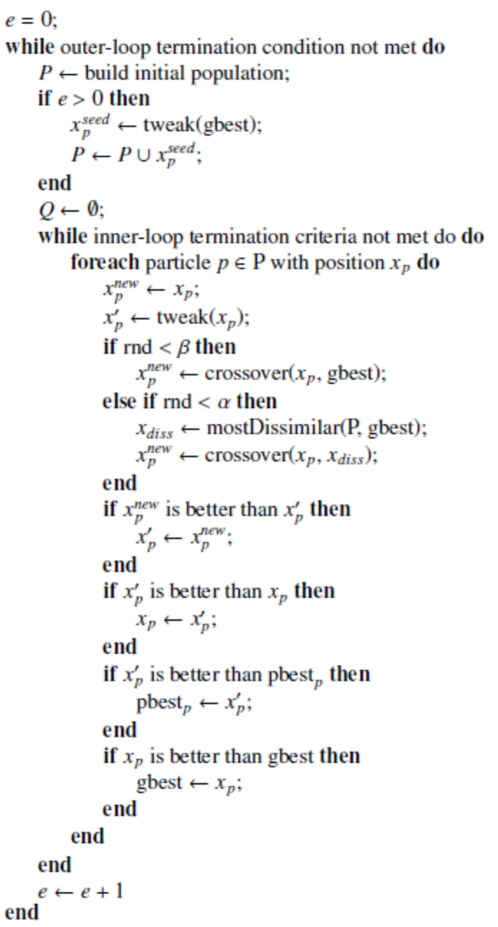
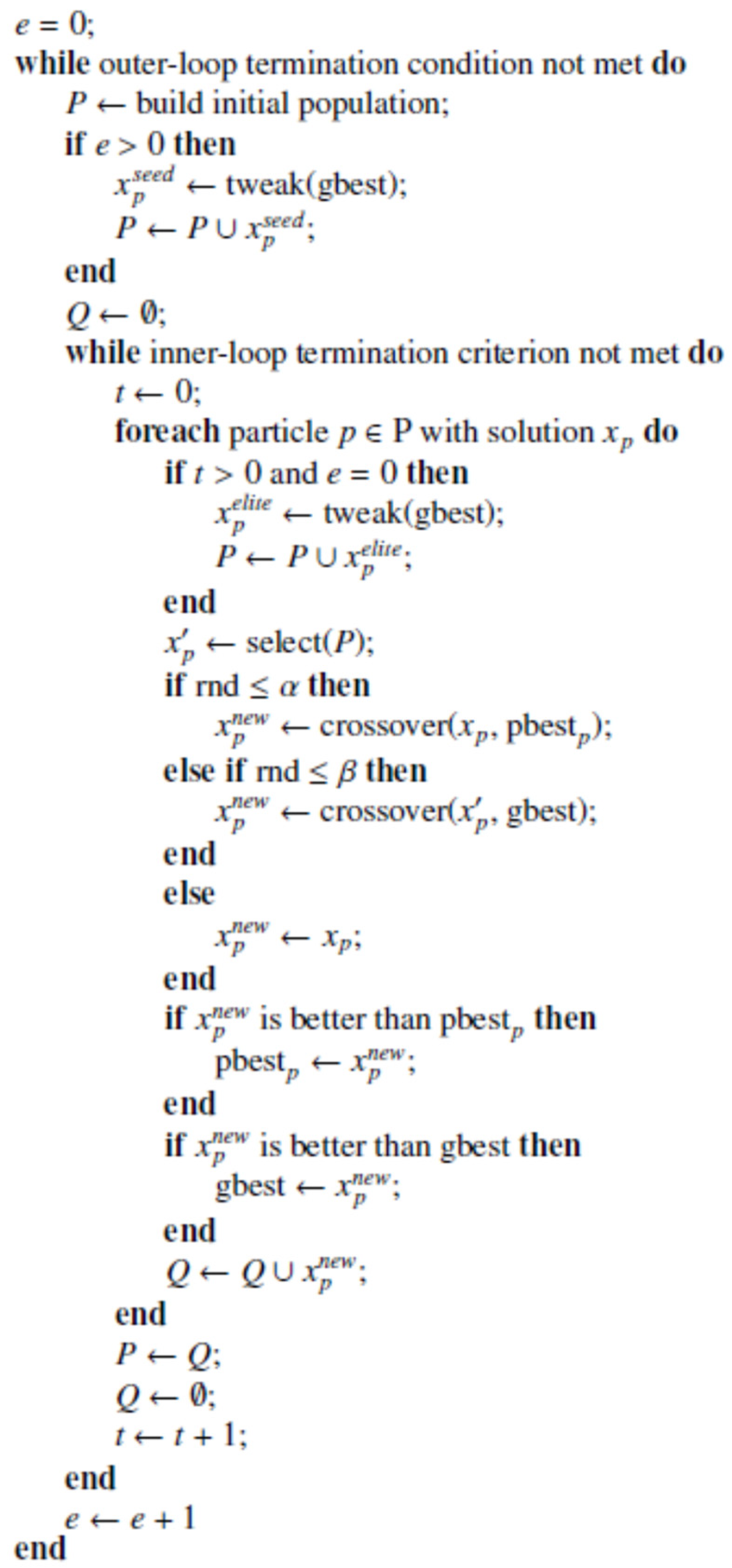
The first step involves generating a sampling plan, denoted as ${\mathit{X}}_s$, which comprises an initial set of samples representing values for the decision variables. The sampling plan can be represented as ${\mathit{X}}_s={\left[{\mathit{x}}_1 {\mathit{x}}_2 \dots {\mathit{x}}_1\right]}^T$, where the vector represents a sample in which each element represents a decision variable. These samples must be well distributed in the search space to be effective, which can be achieved using different approaches, such as Monte Carlo sampling (MCS), Latin hypercube design (LHS), Hammersley sequence sampling (HSS), and orthogonal array sampling (OAS) [27]. The objective of various sampling strategies, often called design of experiments (DoE), is to choose specific points within the design space to optimize information acquisition for each simulation run while concurrently minimizing the time required for sampling [13]. This paper applied the LHS method due to its simplicity and computational speed. Once the initial sampling plan was obtained, the building model was then simulated for each sample in the sampling plan. Each sample, ${\mathit{x}}_i\in {\mathit{X}}_s$, and its simulation value,$y_i\in {\mathit{Y}}_a$, was considered a sampling point. Altogether, the sampling points constitute the dataset $\left({\mathit{X}}_s,{\mathit{Y}}_a\right)$, which was used to train the surrogate model. Following this, a loop was initiated, wherein the next sampling point is selected by minimizing the acquisition function, which the surrogate model defines. Moreover, the termination criterion is the maximum number of iterations, which was set to 50 in all experiments.

Two metaheuristic optimization algorithms, MEPSO-I and MEPSO-II, detailed in Section 2.1.2, were employed to optimize the acquisition function. MEPSO-I and MEPSO-II denote internal optimization algorithms in MEVO-I and MEVO-II, respectively. If a sample has not been simulated, a simulation is executed on that sample, producing an output, y_i,, and the sample is added to the sampling plan,${\mathit{X}}_s$. A new surrogate model was generated when new samples were added to the sampling plan. If the sample obtained with the acquisition function was already simulated, its objective function value, y_i, is retrieved from memory, and the sampling point is included in the surrogate model. Following this, two evolutionary operators, crossover and mutation, were applied based on their given probabilities to generate the new sampling points. The best solutions were ranked as a preliminary step for crossover, and two-parent solutions were selected among the best n solutions. The crossover operator combines these two solutions and generates a new solution if a random number is less than a given probability, $P_{cross}$. Subsequently, if a random number is less than a given probability, $P_{mut}$, a mutation was carried out on the best solution obtained by that point, generating a new solution. The loop was then repeated until the termination criterion was reached.

2.1.2. MEPSO

The micro evolutionary particle swarm optimization (MEPSO) algorithm is derived from the traditional particle swarm optimization (PSO) algorithm [26]. While MEPSO retains the concept of particles imitating swarm behavior, it introduces a different approach to updating particle positions. Thus, instead of using velocity vectors, MEPSO employs crossover operations to calculate new particle positions. The algorithm incorporates MEPSO in its iterative process. The MEPSO algorithm, similar to the micro-genetic algorithm mentioned by the authors of [28], employs a small population size. This choice offers several advantages, including faster convergence and reduced memory usage for storing the population. Each particle in MEPSO retains its current solution, current fitness, and the best solution it has found so far (referred to as $p_{best}$), following a similar structure to the PSO algorithm.

The MEPSO algorithm consists of two nested loops. The outer loop implements an elitist restart, where a new population is created, the optimal individual from the inner loop is transferred, and then the inner loop is restarted. The initial population is created in the first epoch, and the inner loop is initiated. A new population is created before restarting the inner loop for subsequent epochs. The optimal solution in the previous epoch is modified using a real-valued mutation and copied to a randomly selected particle in the new population.

The mutation in MEPSO introduces a variation in solutions by incorporating a random value into one of its elements. The applied mutation technique is the pseudo-Gaussian mutation, wherein instances of zero deviation are more commonly encountered than instances of non-zero deviation. This approach means that the mutation usually results in a slight modification around the existing solution, but occasionally, it may introduce a more significant change. Assuming a solution $\mathit{x}=\left(x_1,\dots ,x_n\right)$, the mutation modifies $\mathit{x}$ into ${\mathit{x}}^{\prime }$ using the below formula in Equation (1):

$$\forall x_i,{\mathit{x}}_i^{\prime }{}^{}=\{\begin{array}{cc}{x}_i& \mathrm{if} r>\mu \\ x_i\cdot \sigma \cdot random\left(0,1\right)& \mathrm{if} r\le \mu \end{array}$$

(1)

where $\sigma$ and $\mu$ are parameters for the real numbers’ mutation sampled between 0 and 1.0, and $r$ is a random number. The epoch was incremented and repeated if a termination condition had not been met.

Two variations of the algorithm have been developed: MEPSO-I and MEPSO-II. The pseudocode for MEPSO-I and MEPSO-II can be found in Figure 2 and Figure 3, respectively. One distinction between MEPSO-I and MEPSO-II pertains to the initial population generation process. MEPSO-I generates the initial population based on the entropy diversity criterion mentioned by the authors of [29], while MEPSO-II employs the Latin hypercube sampling (LHS) method. MEPSO-II implements an elitism strategy for the first epoch, where the optimal solution in the previous iteration is carried over to the next one [30].

Furthermore, the algorithm uses $\alpha$ and $\beta$ as control parameters within its internal loop for enhanced convergence. If a random number between 0 and 1 is less than α, a crossover (α crossover) occurs between the current particle’s solution and the subsequent solution:

• The solution of the most dissimilar particle compared to the best global solution of the swarm (in the case of MEPSO-I).
• The best solution that the particle has discovered so far ($p_{best}$) (in the case of MEPSO-II).

The Euclidean distance determines the most dissimilar solution from the optimal global solution. The solution with the largest Euclidean distance from the best global solution is identified as the most dissimilar by comparing all particles in the population. If $\alpha$ crossover did not occur, and if $\beta$ is greater than a randomly generated number between 0 and 1, a crossover is executed between the solution of the particle and the subsequent solution:

• The best global solution of the swarm (in the case of MEPSO-I).
• A solution of a particle selected with the tournament selection method, as described by the authors of [30] (in the case of MEPSO-II).

The crossover operation was performed using the following procedure. For a real variable,${\mathit{x}}_i\in \left[a_i,b_i\right]$, given two solutions,${\mathit{x}}_1=\left(x_{11},\dots ,x_{1n}\right)$ and ${\mathit{x}}_2=\left(x_{21},\dots ,x_{2n}\right)$, the crossover generates two offspring solutions, ${\mathit{y}}_1=\left(y_{11},\dots ,y_{1n}\right)$, and ${\mathit{y}}_2=\left(y_{21},\dots ,y_{2n}\right)$. This crossover was executed based on the blend method [31], and follows the following formula in Equation (2):

$$\begin{gathered} y_{1i}={\mathsf{\delta }}_i{x}_{1i}+\left(1-{\mathsf{\delta }}_i\right)x_{2i} \\ {y}_{2i}=\left(1-{\mathsf{\delta }}_i\right)x_{1i}+{\mathsf{\delta }}_i{x}_{2i} \end{gathered}$$

(2)

where $\mathsf{\delta }$ is formulated as $\mathsf{\delta }=\left(\mathrm{random}{\left(-\mathsf{\gamma },1+\mathsf{\gamma }\right)}_1,\dots ,\mathrm{random}{\left(-\mathsf{\gamma },1+\mathsf{\gamma }\right)}_n\right)$. If the formula produces values outside of the allowed range $\left[a_j,b_j\right]$, the offspring is adjusted according to the following rules in Equation (3):

$$\begin{array}{c}\mathrm{if} y_{ij}<a_{j, \mathrm{set} }{y}_{ij}=a_j\\ \mathrm{if} y_{ij}>b_{j, \mathrm{set} }{y}_{ij}=b_j\end{array}$$

(3)

If the current solution of a particle surpasses its $p_{best}$, the $p_{best}$ is updated accordingly. Subsequently, if the solution of a particle demonstrates a fitness value better than that of the best global particle, the best global particle is substituted with the particle mentioned above.

2.2. Problem Formulation

To accurately determine the present value of expenses and incomes over a retrofit lifespan, it is essential to consider both the energy price escalation and discount rates. By incorporating these factors, the calculations can be performed with increased precision. The present value calculations encompass the costs associated with natural gas and electricity. The objective function minimizes the lifecycle cost of the retrofit. Therefore, the best solution is found by minimizing the lifecycle cost, as expressed by Equation (4):

$$\min LCC=I+q{U}_{cost}$$

(4)

where $LCC$ represents the net present value of cash flows; $I$ is the investment cost of the retrofit; $q$ is a present value factor; and $U_{cost}$ is the total cost of electricity and natural gas per year calculated based on Equation (5):

$$U_{cost}=p_{e}E+p_{g}G$$

(5)

where $E$ is the electricity consumption in J/year, $G$ is the natural gas consumption in J/year, $p_e$ is the electricity price in $/J, and p_g is the natural gas price in $/J. Both $E$ and $G$ are calculated using the building performance simulator, using the values of insulation thickness of the walls, the U-value, and the solar heat gain coefficient (SHGC) of the windows as decision variables. Then, the annual total heat transfer is used to estimate electricity and natural gas consumption. q is based on the geometric gradient present value factor calculated through Equation (6):

$$q=\{\begin{array}{cc}\frac{\left[1-{\left(\frac{1+g}{1+d_r}\right)}^t\right]}{d_r-g}& \mathrm{if} d_r \ne gr>\mu \\ \frac{t}{1+d_r}& \mathrm{if} d_r=g\end{array}$$

(6)

where $t$ is the life span of the building, $d_r$ is the actual discount rate, and $g$ is the escalation rate through which the energy price increases from one year to the next. $d_r$ is calculated with the nominal discount d_n and the inflation rate e, as shown below in Equation (7):

$$d_r=\frac{1+d_n}{1+e}-1$$

(7)

The necessary data to calculate the lifecycle cost of Equation (4) are shown in

Table 1. Parameters used in the calculation of the objective function.

Parameter	Description	Value
pe	Electricity price in $/kWh	0.143 CAN$/kWh
pg	The natural gas price in $/kWh	0.0135 CAN$/kWh
t	Life span of the building	50 years
dn	Nominal discount	5%
e	Inflation rate	3%
g	Energy price escalation rate	2%

.

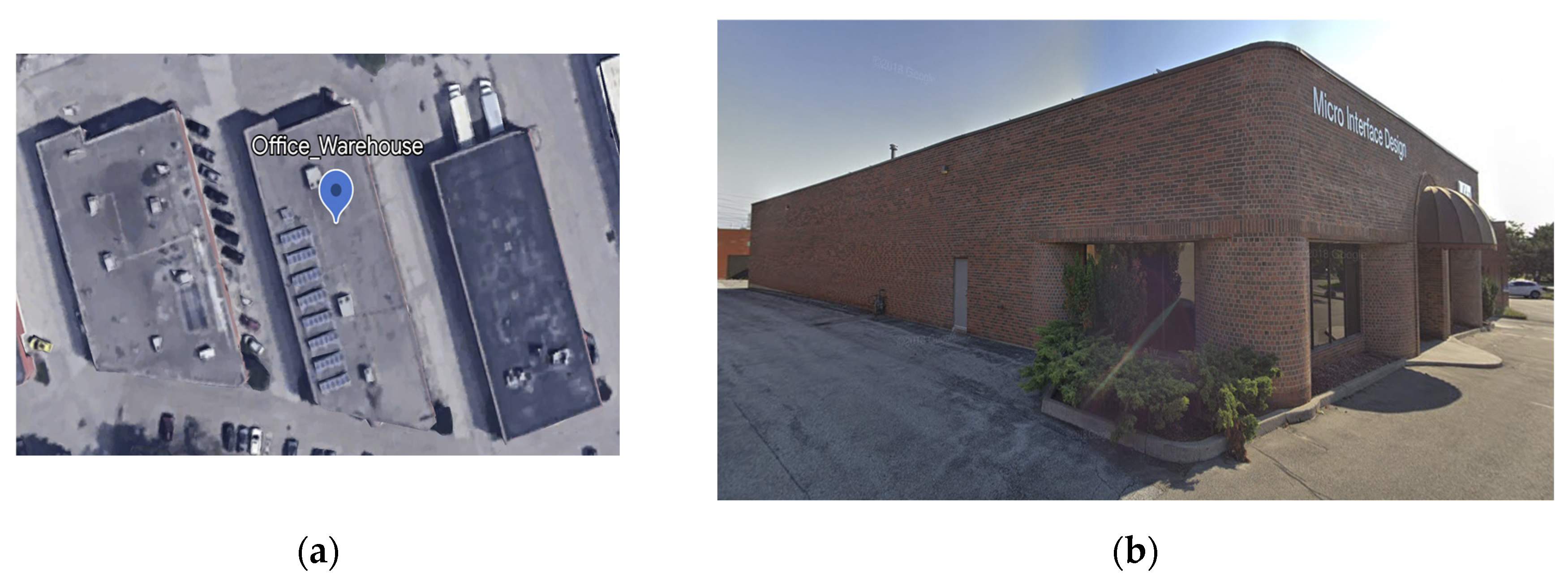
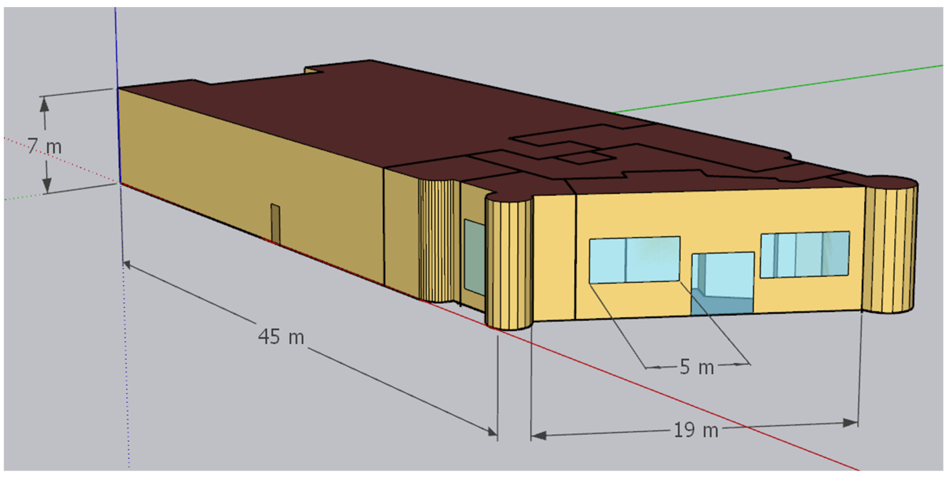
2.3. Case Study Building

The case study is a one-story commercial building in Markham, Ontario, Canada [32] (see Figure 4). It comprises office and workshop space, covering approximately 330 m² and 720 m², respectively, with a 7 m height. The building accommodates 15 people and operates from 10:00 to 18:00 on weekdays. Natural gas is used for space heating and hot water, while electricity is utilized for cooling, lighting, and equipment. Constructed in 1985, before the first building energy code was implemented in 1997 [33], the building’s envelope exhibits poor thermal performance. In this respect, the external walls of the office area are, from the inside to the outside, made of gypsum board, fiberglass insulation, concrete wall, and brick veneer. The workshop area has a similar wall composition but lacks an insulation layer, with an overall thickness of 30 cm. Consequently, the U-value of the office area’s external walls ranges from 1.2 W/m²K to 1.4 W/m²K, while the workshop area’s external walls have a U-value of 2.8 W/m²K, as measured by QEA Tech Company. This poor thermal performance of the exterior walls and windows presents significant potential for energy savings through an energy-efficient retrofit of the building’s enclosure. Additionally, as a typical single-story office building in North America, the retrofit solutions can be applied to similar structures. The gross areas of the windows, doors, and exterior walls are 48 m², 23 m², and 1100 m², respectively.

An eight-zone energy model was developed using SketchUp for geometry and EnergyPlus for dynamic performance simulation to analyze the building’s energy performance (see Figure 5). The workshop area was represented as a single thermal zone, while the office area was divided into seven thermal zones due to variations in its use, orientation, and setpoint temperatures. The necessary data about building characteristics, occupancy profiles, and energy consumption patterns were gathered by conducting surveys, performing building walkthroughs, and analyzing energy bills. The HVAC and domestic heating systems were simulated using OpenStudio, with two packaged rooftop units designated for the warehouse and office areas. The heating coil utilized natural gas with an efficiency of 89%, while the cooling coil was defined as DX single speed with a COP of 3. During occupied hours, the heating setpoint was set to 20 °C in the office area and 17 °C in the warehouse area. For cooling, the setpoint was 22 °C in the office area and 25 °C in the warehouse area during unoccupied hours. Heating setbacks were applied at 16.5 °C and 17 °C for the office and warehouse areas, respectively, while the cooling setback in both areas was set to 26 °C. The hourly annual simulation of the building model took approximately 12 s on a laptop computer equipped with an 11th Gen Intel Core i7-1185G7 CPU of 3 GHz, running Microsoft Windows 10 Enterprise.

2.3.1. Comparison of Simulation Results with Actual Building Energy Consumption

The office building’s natural gas and electricity energy consumption data were available between 25 October 2019 and 13 November 2020, facilitating the assessment of the model predictions. The hourly weather file consisted of actual weather data from January to December 2019 and 2020 obtained from the Government of Canada’s website [34] and solar radiation data sourced from the NSRDB (the National Solar Radiation Database) [35].

After analyzing the energy consumption data, the model was calibrated by adjusting various parameters, such as the R-values of the floor and roof, infiltration, lights, energy consumption, set points, and setbacks. Calibration was conducted following ASHRAE Guideline 14 [36], which requires the normalized mean bias error (NMBE) between measured and modeled monthly energy consumptions to be within ± 5% to ensure confidence in the model’s predictions. The calibrated EnergyPlus model predicted the building’s monthly natural gas and electricity consumption. The NMBE for monthly natural gas consumption was −1.81%, indicating a close match between the calibrated model and the actual data. Similarly, the NMBE for monthly electricity consumption was −0.56%, falling within the acceptable range specified by ASHRAE 14. In addition, the R² was calculated for both natural gas and electricity, with a monthly overall R² of 0.87 and 0.85, respectively.

Notably, the annual percentage error is predominantly driven via natural gas consumption, which exhibited a magnitude of 2.26% compared to a much lower value of 0.77% for electricity consumption. This outcome was expected due to the use of natural gas for space heating and hot water, although the exact ratio was unknown. The calibrated model predicted an annual natural gas consumption of 335,573 kWh/year and electricity consumption of 90,814 kWh/year. The measured natural gas and electricity consumption values were 343,350 kWh/year and 90,120 kWh/year, respectively.

2.3.2. Retrofit Options

The building retrofitting optimization problem consists of minimizing the lifecycle cost of the retrofit through three retrofit options as decision variables (insulation thickness, window U-factor, and SHGC) of the optimization process, presented in

Table 2. Lower and upper values of the decision variables.

Decision Variable	Lower Value	Upper Value
The thickness of the insulation material (m)	0.0252	0.127
Window’s U-factor (W/m2K)	1.3	1.8
Solar heat gain coefficient	0.1	0.3

. The insulation material has a conductivity of 0.03628 W/mK, a density of 176 kg/m³, a specific heat capacity of 176 J/kgK, a thermal absorbance of 0.9, a solar absorptance of 0.7, and a visible absorptance of 0.7.

2.4. Algorithm Evaluation

The performance evaluation of the proposed algorithm was conducted by comparing it against metaheuristic algorithms, namely MEPSO-I, MEPSO-II, GA, and PSO, and Bayesian optimization, which was implemented using the EGO (efficient global optimization) algorithm. For each test of the algorithms, 30 independent runs were conducted. The optimization solution, optimum cost, and computation time were recorded for each run. Subsequently, the solution’s worst, best, mean, standard deviation and average computation time were calculated based on the 30 runs. The optimizer calculated the lifecycle cost (LCC) using the cooling and heating consumption values derived from EnergyPlus. The following overall performance indicators were utilized to evaluate the performance of the algorithms:

• Mean best cost (MBC)—represents the average of the final or best cost observed in the last population across all runs.
• Worst cost (WC)—indicates the highest cost observed among all runs.
• Best cost (BC)—represents the lowest cost observed among all runs.
• Standard deviation (SD)—measures the variability of the final or best cost observed in the last population across all runs.
• Mean computation time (MCT)—denotes the average processing duration in minutes across all runs.

In all runs of MEVO-I and MEVO-II, 50 samples were generated using LHS and then simulated. The resulting samples were utilized to construct a neural network, with the LHS samples as inputs and the lifecycle cost values as outputs. The outcomes of the 50 simulations were stored in a file for later use in the 30 runs. The initial 50-sample generation process took 9.078 min. The neural network employed in this study is a multi-layer perceptron (MLP) neural network created using the Scikit-learn library [37]. The weights and biases of the neural network were determined using the limited memory Broyden–Fletcher–Goldfarb–Shanno (LBFGS) algorithm. The selection of training of the neural network architecture was achieved by varying the number of neurons in the hidden layer from 1 to 12, utilizing the dataset from the initial 50 simulations. In all cases, the logistic sigmoid function was employed as the activation function for the hidden layer. The neural network’s performance, generated with the initial sampling points, was evaluated using the mean square error (MSE) and R² for the whole dataset from the initial 50 simulations. Figure 6 presents the performance of different numbers of neurons in the hidden layer. Although the architecture with the lowest MSE suggests a superior model, the best results were obtained with eight neurons in the hidden layer, yielding an MSE of 3.13 × 10⁻⁴ and an R² value of 0.995. The architecture of the neural network remained constant throughout the iterations of the algorithm, but the neural network model was updated after adding the sampling points using the acquisition function and evolutionary operators. An analysis of the quantitative adequacy of the surrogate model demonstrated that it accurately described the original simulation data in all iterations. During each iteration, whenever a new surrogate model was generated, the root mean square error (RMSE) and R² were used as goodness-of-fit measures. The average RMSE and R² values for MEVO-I were 0.0176 and 0.9941, while for MEVO-II, the corresponding average values were 0.0188 and 0.9931, respectively. These results confirm the suitability of the surrogate model in replicating the original simulations throughout the iterations of the 30 runs.

Table 3. Parameter settings of algorithms MEVO, MEPSO, GA, and PSO.

Algorithm	Parameter
MEVO-I	The maximum number of iterations	50
	Probability of crossover	0.1
	Probability of mutation	0.1
	MEPSO integrated into MEVO
	Alpha	0.6
	Beta	0.9
	Maximum number of epochs	5
	Maximum number of internal loop iterations	5
	Individuals in the internal loop	20
MEVO-II	The maximum number of iterations	50
	Probability of crossover	0.1
	Probability of mutation	0.1
	MEPSO integrated into MEVO
	Alpha	0.02
	Beta	0.96
	Maximum number of epochs	5
	Maximum number of internal loop iterations	10
	Individuals in the internal loop	20
MEPSO-I	The maximum number of epochs	1
	Maximum number of internal loop iterations	7
	Individuals in the internal loop	20
	Alpha 1	0.6
	Beta 2	0.9
MEPSO-I	The maximum number of epochs	4
	Maximum number of internal loop iterations	5
	Individuals in the internal loop	20
	Alpha 2	0.02
	Beta 2	0.96
PSO	Inertia weight 2	0.8
	Cognition coefficient	2.05
	Social coefficient	2.05
	The termination criterion	Maximum of 25 iterations with 20 particles
GA	Crossover fraction	0.5
	Mutation fraction	0.5
	Population size	50
	Generations	30

¹ The values of alpha and beta were obtained by optimizing the Biggs EXP4 function [38] with 80 samples generated with LHS. ² The velocity equation described by the authors of [39] was implemented using the described parameters for PSO in Table 3, which were recommended by the authors of [35].

summarizes the parameters of the optimization algorithms used in this study. These parameters ensure a good trade-off between reliability and computational burden. Moreover, the convergence of distinct algorithms varies according to their respective structures, necessitating different numbers of iterations. Utilizing the MEVO approach offers a distinct advantage in reducing the need for extensive EnergyPlus simulations by leveraging surrogate models.

3. Results and Discussion

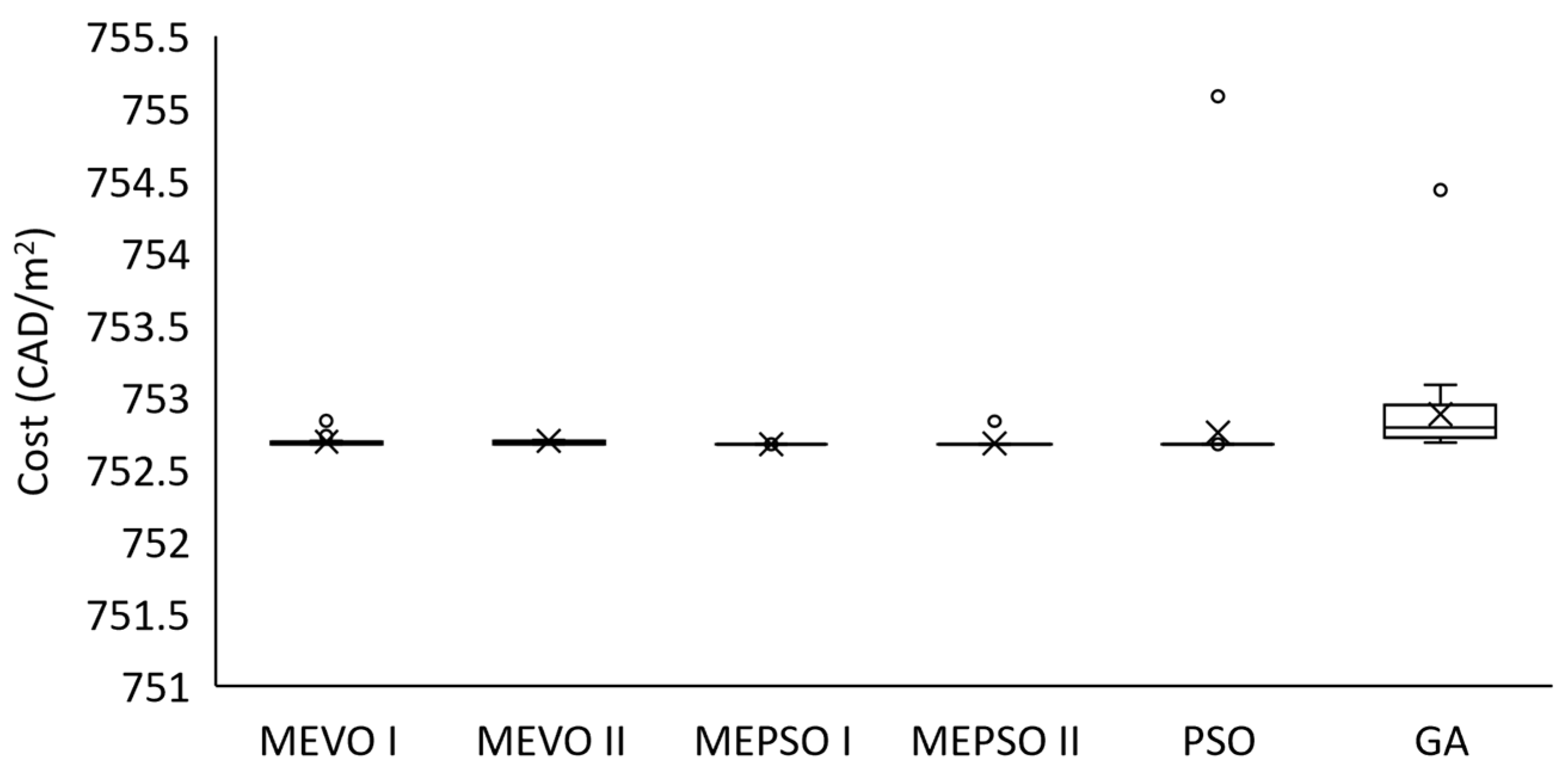
3.1. Comparison between MEVO and Metaheuristic Optimization Algorithms

Comparisons between MEVO and the metaheuristic optimization algorithms MEPSO I and II, PSO, and GA were conducted in the following analyses.

Table 4. Comparison of the performances of MEVO-I and MEVO-II with the metaheuristic optimization algorithms.

	MEVO-I	MEVO-II	MEPSO-I	MEPSO-II	GA	PSO
MBC (CAD/m2)	752.6928	752.6986	752.6746	752.6807	752.8825	752.7562
Best cost (CAD/m2)	752.6740	752.6741	752.6740	752.6740	752.6873	752.6741
Worst cost (CAD/m2)	752.8377	752.8558	752.6876	752.8335	754.4349	755.0850
Standard deviation (CAD/m2)	0.0333	0.0506	0.0025	0.0291	0.3176	0.4398
Mean computation time (min)	13.412 +9.078	11.8871 +9.078	81.3136	89.1136	110.6959	99.2034

presents the optimization algorithms’ average, best, worst, and standard deviation (SD) of the solution cost and the average computation time. Additionally, Figure 7 illustrates the boxplots that compare the cost distributions. The results indicate that the MEVO algorithms yield a solution quality similar to the metaheuristic optimization algorithms, as indicated by their mean best cost (MBC), best cost (BC), and standard deviation. The comparison of cost distributions among the algorithms, as illustrated in Figure 7, reveals that MEVO-I and II display solution variances similar to the metaheuristic algorithms, except for GA, which displays the most significant variance.

On the other hand, the MEVO algorithms were four to six times faster than the other algorithms. It should be emphasized that the additional 9.078 min (see Table 4) was only applied to the first run, which involves the generation of the initial 50 samples used for constructing the initial neural network. These findings indicate that even with fewer simulations, the MEVO algorithms are likely to achieve lower cost values than the metaheuristic algorithms, all while requiring significantly less computation time. The lower computational time of MEVO algorithms can be attributed to their inherent nature compared to the metaheuristic algorithms. Indeed, MEVO saves significant computational time by avoiding extra simulations by utilizing a surrogate model and its unique iterative learning mechanisms. In contrast, MEPSO I, II, GA, and PSO only explore the solution space through the execution of the building performance simulation on each solution.

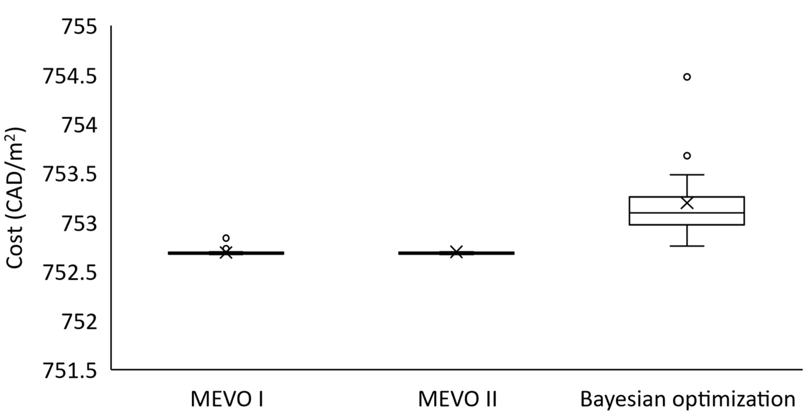
3.2. Comparison between MEVO and Bayesian Optimization

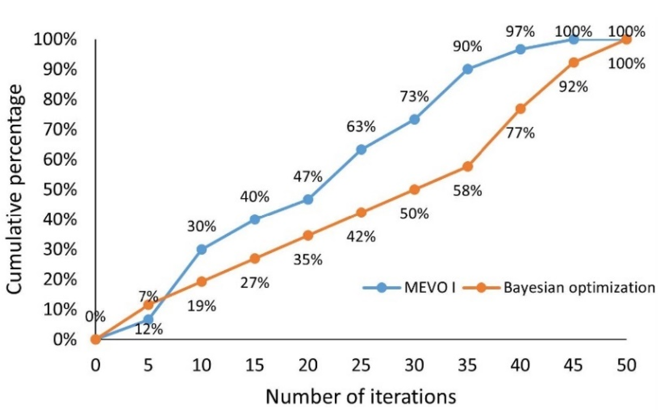
Section 3.1 showed how MEVO, a surrogate-based optimization algorithm, produces a solution quality similar to metaheuristic algorithms in less time. Here, we compare MEVO against Bayesian optimization, a widely used surrogate-based optimization algorithm that, similar to MEVO, implements the iterative approach.

Table 5. Performance of MEVO and Bayesian optimization.

	MEVO-I	MEVO-II	Bayesian Optimization
MBC (CAD/m2)	752.6928	752.6986	753.1964
Best cost (CAD/m2)	752.6740	752.6741	752.7597
Worst cost (CAD/m2)	752.8377	752.8558	754.4766
Standard deviation (CAD/m2)	0.0333	0.0506	0.4039
Mean computation time (min)	13.412 +9.078	11.8871 +9.078	11.8684 +9.078

and Figure 8 compare MEVO with the Bayesian optimization algorithm called EGO. EGO employs a Gaussian process to construct a surrogate model and selects new sampling points based on maximizing the expected improvement function. The expected improvement function is maximized in each iteration to identify the next sampling point. The energy simulation model is then executed at the new sampling point, and the surrogate model is updated to incorporate the results. The Gaussian process implementation utilizes the Gaussian process regressor from Scikit-Learn, using default parameters.

In Bayesian optimization, the number of additional simulations corresponds to the number of iterations. Therefore, to compare MEVO with Bayesian optimization, the number of iterations was set to match the average number of additional simulations in the proposed algorithms, which was 60 for both MEVO-I and II. All the parameters of the Bayesian optimization were kept constant for all 30 independent runs conducted to test each algorithm. As before, the optimization solution, optimum cost, and computation time were recorded for each run. With the initial sampling plan construction time of 9.078 min, both algorithms showed a close computational time, as shown in Table 5. The similarity in computational time was attributed to the number of additional simulations in MEVO being similar to that of Bayesian optimization. The number of simulations added via the crossover and mutation mechanisms is offset by the filter that checks whether the sample has already been simulated so that its objective–objective function is retrieved from memory, not from the BPS. Regarding the MBC, MEVO-I yielded better results than Bayesian optimization. Moreover, regarding solution distribution, Bayesian optimization exhibited more scattered results than the MEVO algorithms, as depicted in Figure 8, meaning that MEVO presents more repeatability, reducing the burden of running the algorithm many times.

A left-tailed Wilcoxon rank-sum test was conducted to assess the significance of the results between MEVO and Bayesian optimization. This test aimed to determine whether MEVO exhibits a significantly better solution quality in the 30 runs than Bayesian optimization. Left-tailed p-values were calculated to test the hypothesis that the median of MEVO is lower than Bayesian optimization’s (BO) median. The Wilcoxon rank-sum test between MEVO-I and BO yielded a p-value of 1.9394 × 10⁻¹¹, while the test between MEVO-II and BO yielded a p-value of 3.5170 × 10⁻¹¹. A 5% threshold was applied to assess the significance level to determine whether the MEVO algorithms demonstrate a statistically significant improvement over Bayesian optimization. The test results indicated that MEVO I and II exhibit a significantly better solution quality, as their p-values are smaller than 0.05. In other words, the alternative hypothesis (H₁: A < B) was supported, confirming that the observations from MEVO (A) tend to be lower than the observations from Bayesian optimization (B). The better solution quality of MEVO over Bayesian optimization can be attributed to the crossover and mutation mechanisms present in the former but absent in the latter.

It is worth mentioning that the results also indicated that the Bayesian optimization algorithm yields similar mean best cost (MBC), best cost (BC), worst cost (WC), and standard deviation (SD) values compared to GA and PSO. However, unlike MEVO, Bayesian optimization exhibits a poorer performance than MEPSO I and MEPSO II. As discussed by the authors of [20], convergence analysis is valuable for evaluating how rapidly an algorithm approaches the optimal solution and determining the relevance of continuing the improvement process after a certain number of iterations.

The following methodology was employed to assess and compare the rate of convergence of both algorithms:

• Calculation of the convergence index $\left(c_{i,j}\right)$ as per Equation (8):

  $$c_{i,j}=\frac{y_{i,j}}{{\overline{y}}_i}$$

  (8)

  where c_i,j represents the convergence index for iteration i within a specific run j, y_i,j denotes the best objective function value achieved up to iteration i in run j, and ${\overline{y}}_{i }$ signifies the mean of the objective function values obtained within run j.
• Determination of the iteration at which convergence is achieved using Equation (9):

  $$t_j^{conv}=min\left\{t_{1,j},\dots ,t_{max}\right\}$$

  (9)
• Subsequently, compute the frequency distribution of t_j values for run j = 1 to j = t_max and the corresponding cumulative percentages using bins of size five.

Figure 9 illustrates the cumulative percentage frequencies concerning the number of iterations. It is clear that for MEVO-I, 90% of the runs reach convergence before the 35th iteration. In contrast, with Bayesian optimization, only 58% of the runs achieve convergence before the 35th iteration. Moreover, when Bayesian optimization achieved convergence in 77% of the runs, MEVO achieved convergence in 97% of the runs. While decreasing the number of iterations in MEVO has a relatively minor impact on the average solution quality, it reduces the time required for the optimization process.

3.3. Scenario Analysis

The solution yielding the best lifecycle cost of 752.6740 CAD/m² was achieved using MEVO-I, as indicated in Table 4 and Table 5. This solution involves incorporating an insulation layer with a thickness of 0.0493 m, installing windows with a U-value of 1.3 W/m²K, and a solar heat gain coefficient (SHGC) of 0.1. The monthly electricity and natural gas consumption before and after the retrofit are compared in Figure 10 and Figure 11. Notably, the retrofit resulted in significant natural gas savings during the coldest months, specifically from December to February. The observed outcome can be attributed to the effective prevention of heat losses, achieved through additional insulation and the installation of high-performance windows. Moreover, the most substantial electricity savings occurred from June to August due to the reduced demand for space cooling resulting from the lower SHGC and U-value of the windows.

It has been highlighted that the MEVO framework is characterized by the effective utilization of artificial neural networks, enabling higher computational capabilities compared to typical metaheuristic algorithms. Consequently, due to the decreased number of required simulations, the reduced computational burden enables the investigation of a wide range of scenarios. Accordingly, this study explored different scenarios by adjusting the project’s lifespan from 20 years to 50 years (the average lifetime of a building varies from 30 years to 50 years for commercial buildings, but low-quality construction can reduce it [2]) and the discount rate from 3% to 10%.

Table 6. Solutions and energy consumption reduction for different values of the project lifespan.

Life Span (years)	Insulation (m)	Window U-Value (W/m2K)	SHGC	Natural Gas Consumption (kWh)	Electricity Consumption (kWh)	Natural Gas Consumption Reduction	Electricity Consumption Reduction
20	0.0254	1.3000	0.1000	306,390.8615	80,531.0916	8.70%	11.32%
30	0.0317	1.3000	0.1000	301,558.3723	79,842.1703	10.14%	12.08%
40	0.0391	1.3000	0.1000	297,064.1325	79,203.8643	11.48%	12.78%
50	0.0493	1.3000	0.1000	292,286.1111	78,579.7222	12.90%	13.47%

and

Table 7. Solutions and energy consumption reduction for different discount rates.

Discount Rate (years)	Insulation (m)	Window U-Value (W/m2K)	SHGC	Natural Gas Consumption (kWh)	Electricity Consumption (kWh)	Natural Gas Consumption Reduction	Electricity Consumption Reduction
3%	0.0711	1.3000	0.1000	285,227.7778	77,651.3889	15.00%	14.49%
5%	0.0493	1.3000	0.1000	292,286.1111	78,579.7222	12.90%	13.47%
7%	0.0341	1.3000	0.1000	299,961.6717	79,616.0683	10.61%	12.33%
10%	0.0254	1.3000	0.1000	306,390.8615	80,531.0916	8.70%	11.32%

provide an overview of the outcomes of the solutions, including natural gas and electricity consumption and respective changes compared to the base case, corresponding to different project lifespans and various discount rates.

These findings indicate that the change in discount rate has a more pronounced impact on energy consumption than the change in lifespan. Specifically, when the discount rate was lowered to 3%, the resulting solution exhibited higher insulation and more efficient windows than the best solution determined through the lifespan assessment.

The total energy consumption and insulation investment cost were calculated for each solution using the optimization results from all the runs. Figure 12 displays the relationship between the total energy consumption and the insulation investment cost, demonstrating a decrease in the total energy consumption as the insulation investment cost increases. This finding confirms the anticipated behavior of two conflicting objectives.

4. Conclusions and Future Work

The innovative methodology proposed in this study integrates machine learning and optimization through incremental learning, improving the surrogate model within evolutionary optimization. The proposed predictive model was initially trained on a limited set of simulated samples to ensure computational efficiency. However, as the optimization progressed, additional configurations were simulated and subsequently integrated into the training dataset. Consequently, the metamodel undergoes self-updating through an iterative procedure of generating sampling points, enhancing its predictive precision. This study employed an artificial neural network model for prediction alongside a faster PSO variant (MEPSO) for optimization, showcasing heightened efficiency and quicker convergence in contrast to traditional PSO. The incremental learning strategy encompasses three distinct simulation approaches for offspring generation: optimal MEPSO outcome, crossover, and mutation, strategically aimed at reducing the optimization time and enhancing the optimal solution’s convergence. The developed framework was applied to a practical scenario involving an actual commercial building with prevalent Canadian construction technologies, providing valuable insights for stakeholders across both public and private sectors in the building industry. The collective integration of these components contributes to a holistic approach that enriches the building energy optimization field. The proposed methodology involves five key steps: defining and calibrating the model, incorporating retrofit options, formulating the objective function, implementing the MEVO optimization strategy, and evaluating MEVO’s performance against MEPSO, PSO, GA, and Bayesian optimization in the context of building energy retrofit. The results implied the following conclusions for the performed comparison:

• MEVO algorithms are faster than direct optimization using MEPSO-I, MEPSO-II, GA, and PSO. When direct optimization is performed with the metaheuristic optimization algorithms, the computation time ranges from 81.3 min to 110.7 min. In comparison, MEVO ranges from 11.88 min to 13.81 min for the second run and from 20.9 min to 22.5 min for the first run. Shorter computation times allow the decision maker to explore several scenarios in less time, such as the effect of different life spans, discounts, or energy price escalation rates.
• The solution quality of MEVO is similar to results obtained with direct optimization using the metaheuristic optimization algorithms. The results indicate that MEVO yields similar mean best cost (MBC), best cost (BC), worst cost (WC), and standard deviation (SD) values compared to the metaheuristic optimization algorithms used for direct optimization: GA, PSO, MEPSO-I, and MEPSO-II. In comparison, Bayesian optimization only yields similar mean best cost (MBC), best cost (BC), worst cost (WC), and standard deviation (SD) values compared to the GA and PSO.
• MEVO surpasses Bayesian optimization in terms of solution quality. The Wilcoxon rank-sum test indicates that both MEVO-I and II exhibit significantly better solution qualities, as their p-values are considerably smaller than 0.05 (1.9394 × 10⁻¹¹ and 3.5170 × 10⁻¹¹, respectively). The better solution quality of MEVO over Bayesian optimization can be attributed to the crossover and mutation mechanisms in MEVO.
• MEVO presents more repeatability, which reduces the burden of running the algorithm many times. MEVO-I and II display solution variances similar to the metaheuristic algorithms with the lowest variances (MEPSO-I, MEPSO-II, and PSO). Moreover, Bayesian optimization exhibited more scattered results regarding solution distribution than the MEVO algorithms.
• The computational time of MEVO is similar to Bayesian optimization. A possible explanation is that the number of simulations added via the crossover and mutation mechanisms is offset with the filter that checks whether the sample has already been simulated so that its objective function value is retrieved from memory and not from the BPS. However, this must be verified for other case studies where the simulation model takes longer to compute.
• In comparison to Bayesian optimization, MEVO requires fewer iterations to converge. For example, while 58% of the runs converged with Bayesian optimization, 90% of the runs converged with MEVO. In addition, it was observed that when Bayesian optimization achieved convergence in 77% of the runs, MEVO exhibited convergence in 97% of the runs. Decreasing the number of iterations in the MEVO algorithm had a comparatively lesser impact on the mean solution quality while simultaneously reducing the duration of the optimization process.

It should be noted that certain limitations must be recognized, providing a foundation for future investigations. First, the effect of different methods for designing computer experiments that uniformly cover the search space in larger dimensional spaces could be investigated. Second, further algorithm modifications are needed to cope with multi-objective problems and use a mix of discrete and continuous variables. Third, the performance of MEVO was assessed by conducting a comparative study with established algorithms in the field of building energy optimization, including PSO and a GA. A comparison was made between MEVO and MEPSO, a critical element of the MEVO framework. Lastly, MEVO’s performance was contrasted with Bayesian optimization owing to their shared structural characteristics.

Nevertheless, future research could assess how MEVO performs compared to other recently developed iterative algorithms with different structures, such as RBFOpt, to discover algorithmic superiority within specific problem domains. Ultimately, the developed algorithm is characterized by a fast iterative surrogate model structure and offers promising computational capabilities compared to static surrogate models. Accordingly, it lays the foundation for more computationally expensive studies, such as retrofitting other building types with complex structures and more decision variables.

References

1. United Nations Environment Programme; Global Alliance for Buildings and Construction. 2021 Global Status Report for Buildings and Construction towards a Zero-Emissions, Efficient and Resilient Buildings and Construction Sector; Technical Report; Global Alliance for Buildings and Construction: Paris, France, 2021; Available online: https://wedocs.unep.org/xmlui/handle/20.500.11822/34572 (accessed on 16 August 2023).
2. IEA. Energy Technology Perspectives 2020. Available online: https://www.iea.org/reports/energy-technology-perspectives-2020 (accessed on 16 August 2023).
3. IEA. Key World Energy Statistics 2021. Available online: https://www.iea.org/reports/key-world-energy-statistics-2021 (accessed on 16 August 2023).
4. Attia, S.; Hamdy, M.; O’Brien, W.; Carlucci, S. Computational optimisation for zero energy buildings design: Interviews results with twenty eight international expert. In Proceedings of the BS2013: 13th Conference of International Building Performance Simulation Association, Chambéry, France, 26–28 August 2013; Available online: https://www.aivc.org/resource/computational-optimisation-zero-energy-buildings-design-interviews-results-twenty-eight (accessed on 16 August 2023).
5. Ascione, F.; Bianco, N.; Mauro, G.M.; Vanoli, G.P. A new comprehensive framework for the multi-objective optimization of building energy design: Harlequin. Appl. Energy 2019, 241, 331–361. [Google Scholar] [CrossRef]
6. Ciardiello, A.; Rosso, F.; Dell’Olmo, J.; Ciancio, V.; Ferrero, M.; Salata, F. Multi-objective approach to the optimization of shape and envelope in building energy design. Appl. Energy 2020, 280, 115984. [Google Scholar] [CrossRef]
7. Mostafazadeh, F.; Eirdmousa, S.J.; Tavakolan, M. Energy, economic and comfort optimization of building retrofits considering climate change: A simulation-based NSGA-III approach. Energy Build. 2023, 280, 112721. [Google Scholar] [CrossRef]
8. Tavakolan, M.; Mostafazadeh, F.; Eirdmousa, S.J.; Safari, A.; Mirzaei, K. A parallel computing simulation-based multi-objective optimization framework for economic analysis of building energy retrofit: A case study in Iran. J. Build. Eng. 2022, 45, 103485. [Google Scholar] [CrossRef]
9. Melo, A.; Versage, R.; Sawaya, G.; Lamberts, R. A novel surrogate model to support building energy labelling system: A new approach to assess cooling energy demand in commercial buildings. Energy Build. 2016, 131, 233–247. [Google Scholar] [CrossRef]
10. Sharif, S.A.; Hammad, A. Developing surrogate ANN for selecting near-optimal building energy renovation methods considering energy consumption, LCC and LCA. J. Build. Eng. 2019, 25, 100790. [Google Scholar] [CrossRef]
11. Razmi, A.; Rahbar, M.; Bemanian, M. PCA-ANN integrated NSGA-III framework for dormitory building design optimization: Energy efficiency, daylight, and thermal comfort. Appl. Energy 2022, 305, 117828. [Google Scholar] [CrossRef]
12. Chegari, B.; Tabaa, M.; Simeu, E.; Moutaouakkil, F.; Medromi, H. An optimal surrogate-model-based approach to support comfortable and nearly zero energy buildings design. Energy 2022, 248, 123584. [Google Scholar] [CrossRef]
13. Kubwimana, B.; Najafi, H. A Novel Approach for Optimizing Building Energy Models Using Machine Learning Algorithms. Energies 2023, 16, 1033. [Google Scholar] [CrossRef]
14. Gengembre, E.; Ladevie, B.; Fudym, O.; Thuillier, A. A Kriging constrained efficient global optimization approach applied to low-energy building design problems. Inverse Probl. Sci. Eng. 2012, 20, 1101–1114. [Google Scholar] [CrossRef]
15. Tresidder, E.; Zhang, Y.; Forrester, A.I.J. Acceleration of building design optimisation through the use of kriging surrogate models. In Proceedings of the First Building Simulation and Optimization Conference, Loughborough, UK, 10–11 September 2012; Available online: http://apps1.eere.energy.gov/buildings/energyplus/ (accessed on 30 August 2023).
16. Gilan, S.S.; Goyal, N.; Dilkina, B. Active learning in multi-objective evolutionary algorithms for sustainable building design. In Proceedings of the Genetic and Evolutionary Computation Conference 2016—GECCO’16, Denver, CO, USA, 20–24 July 2016; Association for Computing Machinery: New York, NY, USA, 2016; pp. 589–596. [Google Scholar] [CrossRef]
17. Bamdad, K.; Cholette, M.E.; Bell, J. Building energy optimization using surrogate model and active sampling. J. Build. Perform. Simul. 2020, 13, 760–776. [Google Scholar] [CrossRef]
18. Lahmar, S.; Maalmi, M.; Idchabani, R. Multiobjective building design optimization using an efficient adaptive Kriging metamodel. Simulation 2023. [Google Scholar] [CrossRef]
19. Mirzaei, K.; Safari, A.; Jalilzadeh, S.; Mostafazadeh, F.; Tavakolan, M.; Safari, M. Environmental, social, and economic benefits of buildings energy retrofit projects: A case study in Iran’s construction industry. In Proceedings of the Construction Research Congress 2020: Infrastructure Systems and Sustainability, Tempe, Arizona, 8–10 March 2020; pp. 693–701. [Google Scholar] [CrossRef]
20. Yang, X.; Chen, Z.; Zou, Y.; Wan, F. Improving the Energy Performance and Economic Benefits of Aged Residential Buildings by Retrofitting in Hot–Humid Regions of China. Energies 2023, 16, 4981. [Google Scholar] [CrossRef]
21. Li, H.; Gutierrez, L.; Toda, H.; Kuwazuru, O.; Liu, W.; Hangai, Y.; Kobayashi, M.; Batres, R. Identification of material properties using nanoindentation and surrogate modeling. Int. J. Solids Struct. 2016, 81, 151–159. [Google Scholar] [CrossRef]
22. Roman, N.D.; Bre, F.; Fachinotti, V.D.; Lamberts, R. Application and characterization of metamodels based on artificial neural networks for building performance simulation: A systematic review. Energy Build. 2020, 217, 109972. [Google Scholar] [CrossRef]
23. Westermann, P.; Evins, R. Surrogate modelling for sustainable building design—A review. Energy Build. 2019, 198, 170–186. [Google Scholar] [CrossRef]
24. Wortmann, T. Genetic evolution vs. function approximation: Benchmarking algorithms for architectural design optimization. J. Comput. Des. Eng. 2019, 6, 414–428. [Google Scholar] [CrossRef]
25. Jones, D.R.; Schonlau, M.; Welch, W.J. Efficient Global Optimization of Expensive Black-Box Functions. J. Glob. Optim. 1998, 13, 455–492. [Google Scholar] [CrossRef]
26. Solano-Rojas, B.J.; Villalón-Fonseca, R.; Batres, R. Micro Evolutionary Particle Swarm Optimization (MEPSO): A new modified metaheuristic. Syst. Soft Comput. 2023, 5, 200057. [Google Scholar] [CrossRef]
27. Garud, S.S.; Karimi, I.A.; Kraft, M. Design of computer experiments: A review. Comput. Chem. Eng. 2017, 106, 71–95. [Google Scholar] [CrossRef]
28. Batres, R. Generation of operating procedures for a mixing tank with a micro genetic algorithm. Comput. Chem. Eng. 2013, 57, 112–121. [Google Scholar] [CrossRef]
29. Bessaou, M.; Siarry, P. A genetic algorithm with real-value coding to optimize multimodal continuous functions. Struct. Multidiscip. Optim. 2001, 23, 63–74. [Google Scholar] [CrossRef]
30. Luke, S. Essentials of Metaheuristics: A Set of Undergraduate Lecture Notes, 2nd ed.; Lulu: Richmond, VA, USA, 2013; Available online: https://cs.gmu.edu/~sean/book/metaheuristics/Essentials.pdf (accessed on 9 October 2023).
31. Haupt, R.L.; Haupt, S.E. Practical Genetic Algorithms, 2nd ed.; Wiley Interscience: Hoboken, NJ, USA, 2004. [Google Scholar]
32. Dadras, Y.; Kavgic, M.; Alaei, O. Investigation of the thermal transmittances calculated using new infrared technology developed by qea tech. In Proceedings of the 16th Canadian Conference on Building Science and Technology, Vaughan, ON, Canada, 27–28 October 2022; pp. 2014–2023. [Google Scholar]
33. Meacham, B.J.; Associates, M.; Mifiree, C. Performance-Based Building Regulatory Systems: Structure, Hierarchy and Linkages. J. Struct. Eng. Soc. New Zealand 2004, 17, 37–51. [Google Scholar]
34. Historical Data-Climate-Environment and Climate Change Canada. Available online: https://climate.weather.gc.ca/historical_data/search_historic_data_e.html (accessed on 16 August 2023).
35. Sengupta, M.; Xie, Y.; Lopez, A.; Habte, A.; Maclaurin, G.; Shelby, J. The National Solar Radiation Data Base (NSRDB). Renew. Sustain. Energy Rev. 2018, 89, 51–60. [Google Scholar] [CrossRef]
36. American Society of Heating, Refrigerating and Air-Conditioning Engineers. In ASHRAE Guideline 14-2014: Measurement of Energy, Demand and Water Savings, ASHRAE Guideline; American Society of Heating, Refrigerating, and Air-Conditioning Engineers, 2014.
37. Pedregosa, F.; Varoquaux, G.; Gramfort, A.; Michel, V.; Thirion, B.; Grisel, O.; Blondel, M.; Prettenhofer, P.; Weiss, R.; Dubourg, V.; et al. Scikit-learn: Machine Learning in Python. J. Mach. Learn. Res. 2011, 12, 2825–2830. [Google Scholar]
38. Biggs, M.C. Minimization Algorithms Making Use of Non-quadratic Properties of the Objective Function. IMA J. Appl. Math. 1971, 8, 315–327. [Google Scholar] [CrossRef]
39. Sengupta, S.; Basak, S.; Peters, R.A., II. Particle Swarm Optimization: A Survey of Historical and Recent Developments with Hybridization Perspectives. Mach. Learn. Knowl. Extr. 2019, 1, 157–191. [Google Scholar] [CrossRef]
Figure 1. The architecture of the MEVO algorithm.
Energies 16 07026 g001
Figure 2. The architecture of the MEPSO-I algorithm integrated into the MEVO-I algorithm.
Energies 16 07026 g002
Figure 3. The architecture of the MEPSO-II algorithm integrated into the MEVO-II algorithm.
Energies 16 07026 g003
Figure 4. Building map (a) and the actual building (b).
Energies 16 07026 g004
Figure 5. The modeled building in SketchUp.
Energies 16 07026 g005
Figure 6. Performance of different neural networks.
Energies 16 07026 g006
Figure 7. Box plot comparing MEVO-I and MEVO-II with the metaheuristic optimization algorithms. The × and ο show the mean best cost and outliers, respectively.
Energies 16 07026 g007
Figure 8. Box plot comparing MEVO-I and MEVO-II with the Bayesian optimization algorithms. The × and ο show the mean best cost and outliers, respectively.
Energies 16 07026 g008
Figure 9. Cumulative percentage curves of  t j c o n v  values.
Energies 16 07026 g009
Figure 10. Comparison of electricity consumption.
Energies 16 07026 g010
Figure 11. Comparison of natural gas consumption.
Energies 16 07026 g011
Figure 12. The relationship between the total energy consumption and the insulation investment cost.
Energies 16 07026 g012