Hybrid-Model-Based Digital Twin of the Drivetrain of a Wind Turbine and Its Application for Failure Synthetic Data Generation

Abstract

Computer modelling and digitalization are integral to the wind energy sector since they provide tools with which to improve the design and performance of wind turbines, and thus reduce both capital and operational costs. The massive sensor rollout and increase in big data processing capacity over the last decade has made data collection and analysis more efficient, allowing for the development and use of digital twins. This paper presents a methodology for developing a hybrid-model-based digital twin (DT) of a power conversion system of wind turbines. This DT allows knowledge to be acquired from real operation data while preserving physical design relationships, can generate synthetic data from events that never happened, and helps in the detection and classification of different failure conditions. Starting from an initial physics-based model of a wind turbine drivetrain, which is trained with real data, the proposed methodology has two major innovative outcomes. The first innovation aspect is the application of generative stochastic models coupled with a hybrid-model-based digital twin (DT) for the creation of synthetic failure data based on real anomalies observed in SCADA data. The second innovation aspect is the classification of failures based on machine learning techniques, that allows anomaly conditions to be identified in the operation of the wind turbine. Firstly, technique and methodology were contrasted and validated with operation data of a real wind farm owned by Engie, including labelled failure conditions. Although the selected use case technology is based on a double-fed induction generator (DFIG) and its corresponding partial-scale power converter, the methodology could be applied to other wind conversion technologies.

1. Introduction

In modern times, wind energy conversion is one of the most promising and reliable energy technologies. Europe already has 220 GW of wind capacity installed and there are plans to install an additional power of 105 GW over the next five years [1]. Actors involved in this energy source are continuously researching this technology with the aim of achieving the best levelized cost of energy (LCOE). According to WindEurope, operation and maintenance (O&M) expenses account for 25–35% of LCOE of wind turbines [2], where corrective maintenance is responsible for 30–60% of O&M costs [3]. The current potential of digitalization and artificial intelligence (AI) can greatly contribute to the increase in the energy production of wind farms, reducing unplanned interruptions, optimizing O&M, and extending the lifetime of the components.

Wind turbines systems can be classified depending on the type of generator, gearbox and power converter used. A double-fed induction generator (DFIG) with a multiple stage gearbox and a partial scale converter is a widely used technology [4]. In the DFIG topology [5], there is a direct connection between the stator windings and the constant frequency grid while the rotor winding connection to the grid is made through a pulse width modulation (PWM) power converter, using a set of slip rings. The power converters can control the rotor circuit current, frequency, and phase angle shifts [6]. This kind of induction generator can operate in a range of ±30% of synchronous speed, achieving a high energy yield, a power fluctuation reduction and the capability of controlling reactive power. A drawback of the DFIG is the inevitable need for slip rings.

A wind turbine is also equipped with a control system, which is responsible for assuring the correct operation of the wind turbine along its entire power curve and keeping the wind turbine within its normal operating range. Wind turbines contain electrical, mechanical, hydraulic, or pneumatic systems, and require sensors to monitor the variables that determine the required control action. The most common variables sensed in a control system are wind speed, rotor speed, active and reactive power, voltage, and the frequency of the wind turbine’s connection point. Moreover, the control system is responsible for stopping the wind turbine if necessary. One control strategy is the pitch angle control [7], which is a good option for variable-speed operations in wind turbines generating more than 1 MW. Using this control, the blades can be correctly oriented with respect to the wind direction in order to avoid extremal values (too high or too low) of the power output. The pitch system is based on a hydraulic system, which requires a computer system or an electronically controlled electric motor.

There are several studies that analyse the critical failure modes of the wind turbine drivetrain system, specifically the electric generator and power conversion system [8,9,10]. While identifying the sources of failure in the electric generator [11], the typologies of failures can be of different kind. Thermal failures can occur due to the effect that currents and overcurrents circulating through the windings have on the insulation and considering that a maximum temperature is withstood depending on the type of insulation and operating conditions. Electrical failures can also occur due to the peaks of voltage that can be applied to the conductor under normal operating conditions and in anomalous situations, such as surges coming from the converter. Environmental failures can be caused by environmental conditions that could degrade insulating material or create corrosion phenomena. Mechanical failures are mainly caused by vibrations. Finally, thermo-mechanical failures are caused by cyclic operating conditions with sudden or continuous variations in temperature, which have different effects depending on the cable material and its accessories (insulation, screens, etc.). The electric generator and the power converter have a greater impact on the reliability, failure rate, and unavailability of the wind turbine. Their failure rate is 15% per year for the electric generator and 6.8% for power converters of offshore wind farms [12,13]. These components are equipped with sensors (temperature, vibrations, electric parameters and others) and connected to the wind turbine supervisory control and data acquisition (SCADA) and condition-based monitoring (CBM) systems. Thus, a long historical real operation dataset exists for each turbine of a wind farm. Sometimes, this dataset includes recorded anomalies or failure in the operation of the turbine.

Data-driven models extract knowledge from real measurements that apply AI (artificial intelligence) techniques, which analyse large amounts of data to identify meaningful patterns in them. In the field of wind energy generation, there are several approaches for this type of model. For instance, the spectral analysis of current signals has been used for health monitoring of stator and rotor windings, as well as the main bearing of wind turbines [14]. In [15], a data-driven model is directly constructed with the objective of detecting and isolating sensor and actuator failures in wind turbines, while the study of [16] develops a hierarchical bank of negative selection algorithms (NSAs) to detect and isolate common failures in wind turbines. The study of [17] uses a data-driven failure diagnosis and isolation (FDI) method for wind turbines. It consists of the implementation of long short-term memory (LSTM) networks for residual generators. The decision-making process is made by applying a random forest algorithm. These FDI methods are designed using experimental and historical data generated both under normal and failure conditions; therefore, the availability of well-developed databases that include labelled anomaly/failure data is mandatory. The accuracy of data-driven methods is generally poor for cases not included in a training dataset. In addition, black box models (e.g., deep learning models) show a low explainability, making it difficult for domain experts to interpret results and gain the required trust to make decisions based on the output of the models.

As a solution to this main drawback of data-driven models, DTs that use physics-based models are developed to make the DT self-explanatory. The term “digital twin” can be defined as “a virtual representation of a real-life system or asset with the same behaviour”. It allows system states to be calculated using integrated models and data, aiding the decision-making process over its life cycle from design to decommissioning. The concept of DT was first described in David Gelernter’s 1991 book Mirror Worlds [18], and the term “digital twin” was first mentioned in a roadmap report developed by John Vickers (NASA) in 2010. The DT concept consists of two distinct parts: (1) the physics-based model representing the asset and (2) the connection of the model with the real asset. This connection refers to the information transferred (automatically or manually) from the asset to the DT and the information that could be transferred from the DT to the asset and the operator. In this way, a DT can accurately estimate an asset’s condition.

A DT is based on mathematic models that represent physical phenomena, making it possible to understand the behaviour of the real asset in each moment. In addition, using this physics-based model, it is possible to create synthetic data for events that have never happened before, acquiring knowledge of the behaviour in some conditions that in other cases would not be possible. Data-driven models can identify and prevent events that were measured in the past. However, the training process of the data-driven algorithms, either non supervised or supervised, always relies on historical data. DTs, on the contrary, provide two new information sources: firstly, physics-based models can allow us to understand their real behaviour, and secondly, physical simulation enables the generation of synthetic data for potential new scenarios, such as potential anomalies or failure conditions. Moreover, hybrid models, considered to be a combination of physics-based models and data analytics, provide a powerful tool for diagnosis and prognosis [19]. Hybrid models developed with this purpose are a good basis for DT creation.

The main advantage of a DT design for a specific industrial setting is the potential to simulate realistic scenarios that are difficult or costly to create in the real system. These scenarios might be used for the prescriptive analysis of new operating conditions, or for testing extreme conditions and responses to anomalies or failures. The main challenge is to develop a simulation method that can be parametrized to output scenarios that differ from normal operation and, in some cases, to simulate conditions that have never been seen before in the real system. The authors of [20] describe four main approaches for the generation of simulated scenarios based on: (1) a simplified physical model; (2) a more complex DT design to model the specific properties of the real scenario; (3) a parametrized statistical generative model built upon prior knowledge of the relationships between variables; and (4) generative models trained with existing real data distribution.

The methodology proposed in this paper brings together approaches 2 and 4 to develop a hybrid digital twin that combines physics-based models and data-driven models to match a specific operation context, both in normal and extreme or failure conditions. In addition, the DT preserves the constrains, significance and explainability of a physical model, overcoming some of the main limitations of a purely statistical generative model (i.e., generative adversarial networks). The physics-based model for the drivetrain of a wind turbine is developed using MATLAB Simulink R2020b.

The paper is organized as follows: Section 1 describes the developed technical approaches and the literature review related to such technical approaches, as well the problems of using data-driven approaches in comparison with hybrid models. Section 2 explains the proposed methodology for developing a hybrid-model-based digital twin and the advantages of combining both physics-based and data-driven models. Moreover, this section describes the principles of synthetic data generation and how such principles can be applied to failure data generation. In Section 3, this methodology is concretely applied to a use case: the drivetrain of a 1.5 MW wind turbine with DFIG technology. Section 4 contains the conclusions and perspectives of future research.

2. Methodology for a Hybrid Model Creation, Synthetic Failure Data Generation and Failure Classification Applied to a Digital Twin

DT development involves several technical tasks combining domain-specific knowledge and data analytics skills. First, the equipment or system deterministic model in normality conditions (so-called normality model) must be generated (e.g., by simulation model). This process includes the representative modelling of underlying physical phenomena and the rigorous selection of design parameters. Then, the constructed model must be validated using real data in non-failure conditions and optimizing certain model parameters values to increase the model accuracy and representativeness against the real equipment behaviour.

In addition, a DT conceived for failure conditions diagnosis includes a suite of physics-based models able to simulate different anomaly or failure scenarios. These failure models might be used for a cause–effect analysis and to establish condition indicators (CI) and they constitute an excellent basis for real failure conditions synthetic data generation [21]. Finally, machine learning (ML) classification techniques (supervised or non-supervised) might be applied for the diagnosis or early detection of failures. The implementation of all these models and algorithms in a digital platform and their online use constitute a complete DT for anomaly/failure diagnosis.

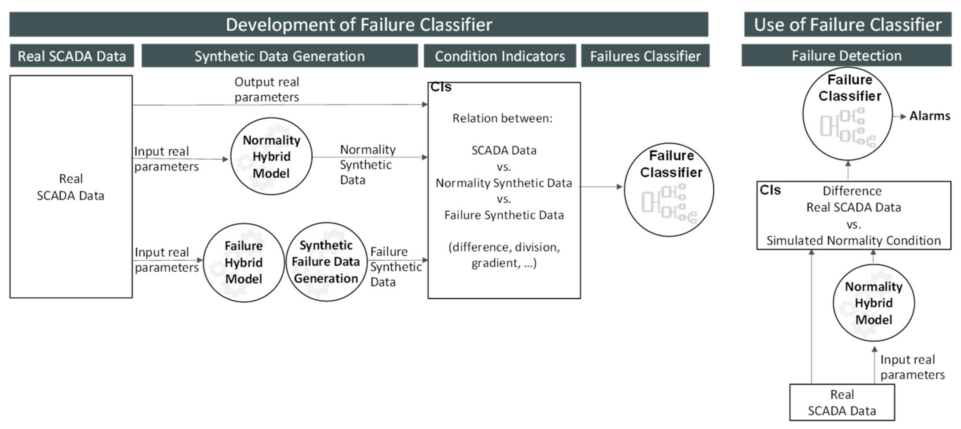
This chapter describes and analyses the methodology for the development and use of an equipment or system DT based on hybrid models for failure classification, making use of a normality hybrid model and a synthetic data generation process. Figure 1 summarizes the whole methodology, and each key component is explained in the following chapters.

2.1. Normality Hybrid Model

The normality hybrid model of the DT is composed of a physics-based model trained with real operation SCADA data in normality conditions.

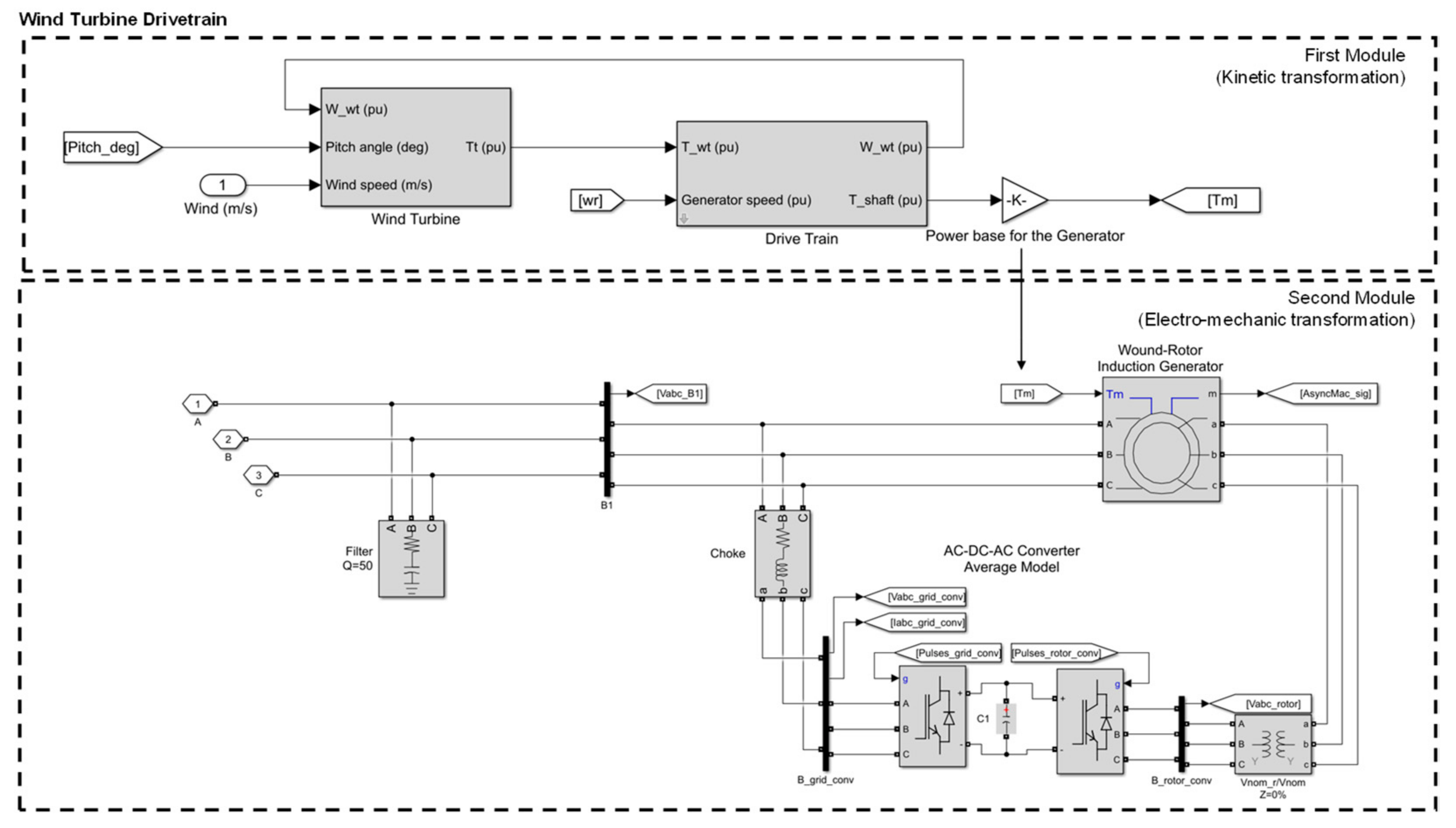
The paper considers the drivetrain of a wind turbine with DFIG technology as a reference use case in which the proposed DT development methodology is illustrated and applied. Figure 2 shows how the physics-based model is divided in two modules that could be used either coupled together or separately, depending on the available operational data. The first module represents the conversion from kinetic energy from the wind to mechanical power, taking the real values of the wind speed measured at the turbine and the pitch angle of the blades as inputs. The second module represents the electro-mechanical conversion. It takes the mechanical torque in the shaft of the DFIG as the input and the generated electric power and its related signals, such as phase currents and voltages or electromagnetic torque, are the outputs. Moreover, this second module includes a power converter and control system that enables the optimal operation of the drivetrain.

The physics-based model is constructed considering the system design parameters. Depending on the nature of the equipment it may be difficult to obtain the complete set of design parameters. In this case, estimations are required, which may impact model performance. Finally, the physics-based model is trained using real operation SCADA data (Figure 3). Training consists of optimizing the values of certain independent design parameters whose exact values are estimated between given realistic intervals.

The objective function of the training process is the minimization of “residue” defined as the difference between the physics-based model output (prediction) and the SCADA real operation data (e.g., output power) for the given real inputs (e.g., wind speed or torque). The resulting calibrated physical model is known as the normality hybrid model.

2.2. Failure Hybrid Model

Once the normality hybrid model is constructed, it can be extended or adapted to include anomaly or failure situations. This new model is called a failure model. Following the same process used in the normality hybrid model, this model is trained using the operation real SCADA data. Similarly, calibration consists of optimizing the values of certain independent design parameters that represent failure, whose exact values are estimated between given realistic intervals.

This resulting new model is also trained with historical and actual operational data of both normal and failure operation. This is achieved using real failure operation data inputs, which are fed to the failure models. In other words, when the normality hybrid model is adapted to represent a failure and trained with failure data (data representing failure operation), the normality hybrid model becomes a failure hybrid model. Feeding the failure models with failure data enables the values of the failure model parameters that define the failure models to be calibrated. The selected values of these failure model parameters are obtained by minimizing the difference between the prediction obtained by the failure model using failure operation data inputs and their corresponding well-known real operation data failure outputs. As a result, the so-called failure hybrid model of the power conversion system (drivetrain) of a wind turbine is obtained, which considers both data of the drivetrain in normal operation and in failure operation.

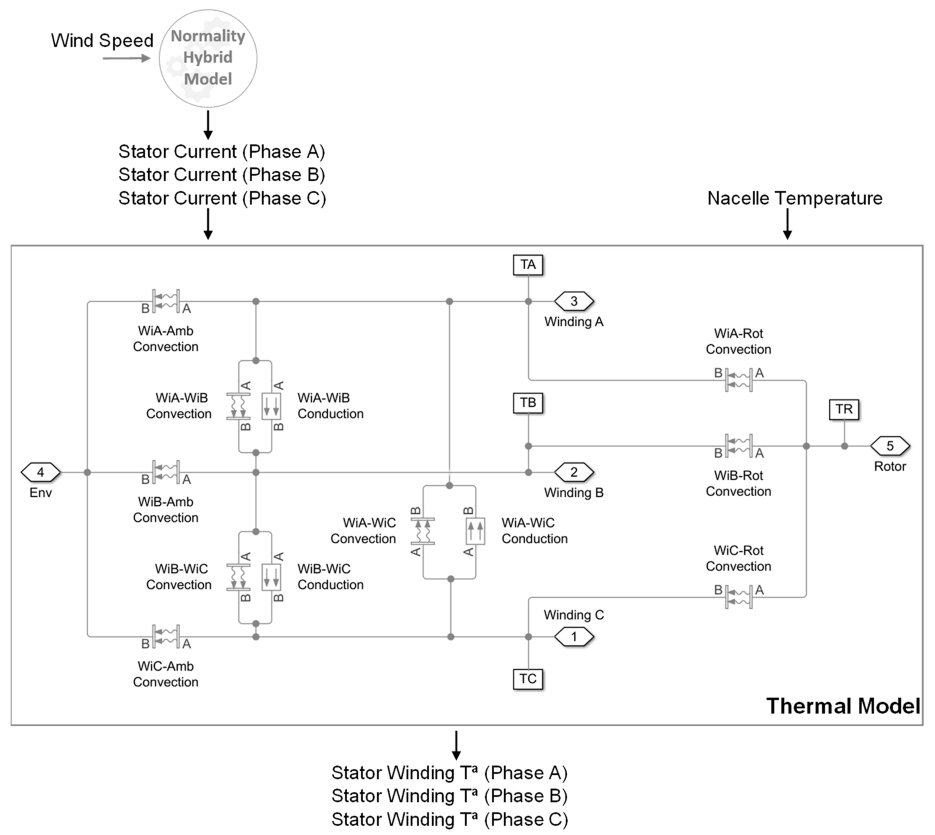
In this case, the overheating of the DFIG stator winding is studied. For this scenario, a thermal model is added to the normality hybrid model (Figure 4).

This thermal model takes as input the real values of the nacelle temperature and the stator phase currents. These values of these stator currents can be estimated by the normality hybrid model or any other value that can be useful for testing the thermal behaviour of DFIG stator windings. The obtained predicted output corresponds to the temperature of the DFIG stator winding.

2.3. Failure Synthetic Data Generation

The methodology analysed in the article has a fundamental contribution in the generation of synthetic data. The generation of synthetic data is a key point because it allows immediate availability of operation data (either normality or failure data), that are difficult to obtain from simple observation of the reality. In addition, the training of classification models for failure prognosis is much enriching using a broad and balanced dataset that represents a variability of behaviour.

Ref. [22] proposes GANs for the generation of synthetic data for wind turbine failure diagnosis research. This article proposes a method to generate synthetic data using the hybrid model and a statistical process. The statistical process characterizes the probability distributions of the occurrence of normal and failure operating scenarios.

The generation of synthetic scenarios in a DT is often deterministic; therefore, the given input data (i.e., wind speed, nacelle temperature and blade pitch angle) always calculate the same output data (i.e., active power, winding temperature, etc.). This process does not consider the variance present in the real data due to factors not modelled by the DT. Hence, the DT does not have the ability to interpolate within the space of the training data and cannot generate truly new scenarios, nor can it include the full extent of the variability observed in the data. In the case of the generation of normal condition scenarios, this determinism is compensated by the amount of training data in such conditions. It is reasonable to assume that these data include a comprehensive range of conditions that represent the entire feature space.

However, this might not be the case for the generation of failure conditions. Although the failure hybrid model has been calibrated to simulate the instances belonging to this type of conditions present in the training SCADA data, this does not guarantee that these instances are a representation of the entire anomalous feature space. In fact, the frequency of anomalous conditions and failures is relatively low in SCADA data, and often these instances are not annotated (labelled). Hence, relaying merely on a deterministic model to generate synthetic failure scenarios would provide a narrow data sample constrain to patterns already seen before.

To resolve this limitation, the DT can incorporate stochastic failure models for the generation of failure scenarios. Each of these models can generate an unlimited number of synthetic failure scenarios for a particular failure type based on real observations in SCADA data.

The corresponding models are trained to approximate the distributions of the variables that define a failure. In addition, some failures cannot be considered instantaneous, but as a pattern in time that leads to a malfunction, a safety stop or a break. This is especially important if synthetic generated failures are to be used to train models that can produce early warnings before a failure is likely to occur.

Both the join probability distribution of the operating variables prior to and during a failure and their physical constrains are initially defined by domain knowledge and can then be updated with observations from real SCADA data. The generation of new failure scenarios is based on random sampling of these probability distribution. Hence, the synthetic scenarios generated by the model are based on real SCADA observations but are not identical to any of those. The process for the synthetic failure data generation of Figure 1 is detailed in Figure 5. It consists of two steps: an observation step and a synthetic data generation step. The observation step aims to identify the probability density function (PDF) that characterizes the failure scenario occurrence. For this, SCADA data are filtered to identify scenarios that correspond to a failure type $f_k$, where k is part of a set of failures K modelled by the DT, such that $k\in K$. A failure scenario is defined by a set of fixed physical constrains defined by domain knowledge and a set of parameters (condition indicators) to be tuned in function of the observed features in failure scenarios from SCADA data.

The PDFs of the parameters are learnt from the observed instances in the SCADA data. These instances might be exclusively sourced from a single turbine or, in case of an insufficient number, they can be sourced from different turbines that share some design and operations characteristics. The decision to include instances from more than one turbine should be made on the basis of turbine similarity and the variability of failure parameters, which depends on operation and design characteristics. The distribution of most parameters might be approximated by a normal PDF with the required precision. However, other distributions might need to be considered for certain parameters. In the case of having access to SCADA data with several instances of a given failure for more than one turbine, a hierarchical parameter modelling might provide a better balance between accuracy and generalization. The learnt PDFs of the parameters are used to update the prior parameter distributions of the corresponding failure model. The data generation process step consists of generating data sets for normality and failure scenarios. As shown in Figure 6, the normality scenario data sets are generated either by running the normality hybrid model or selecting those SCADA data labelled as normal data.

The failure scenario data sets are stochastically generated following the observed and identified PDF, then running and obtaining the results from the failure hybrid model.

2.4. Potential Application of the Hybrid Models Conforming the Digital Twin

The development of data-driven algorithms for diagnosing normality or failure conditions is a complex task that involves: (i) defining the condition indicators (CIs), (ii) labelling normality and failure operation data, (iii) conceptualization of the classification model, (iv) validation of the model (e.g., number of false positives and negatives), and (v) evaluation of the generalization capacity of the model analysing whether it is representative for a set of machines. The DT can add value to this endeavour by providing additional synthetic data to strengthen the dataset.

Figure 7 shows a proposed schema of a supervised classifier training process for failure diagnosis where the explained models in the previous sections are leveraged. The classifier is trained with a labelled dataset composed of real SCADA data, augmented with synthetic data generated via the process described in the previous section.

In addition, the normality hybrid model is used as a baseline to create new CIs that may improve the accuracy of the classifier. These CIs are calculated by comparing real operation SCADA data with respect to synthetic failure data and/or normality data generated by the normality hybrid model.

Finally, Figure 8 shows the execution phase, where CIs are created by comparing real SCADA data with the data simulated by the normality hybrid model. When the values of these CIs meet certain criteria detected by the classifier, an early alarm is generated.

3. Results of Application of the Methodology to a Use Case: 1.5 MW DFIG Wind Turbine

The methodology described in previous section was applied and validated with real SCADA data from a wind turbine in operation owned by Engie. The drivetrain of this wind turbine comprises a 1.5 MW DFIG and its corresponding back-to-back power converter.

Three years of real operational data were organized and preprocessed before use. During the data exploration and pre-processing of SCADA data, relationships between physic parameters were analysed, in order to detect possible outliers, which were removed.

Once the initial data analysis was carried out, the physical model of the power conversion was developed in Simulink-Matlab R2020b (Figure 9). Information on the design parameters of both the generator and power converter was used as a basis for constructing the model. However, some other values were calculated or estimated due to the lack of information. Wind speed and pitch angle are the input parameters needed to operate the model. The result is the generated electric power, currents, and voltages, among others.

The DFIG block implements a three-phase wound rotor asynchronous machine, operating in the generator mode. It uses a fourth-order state-space model to represent the electrical part of the machine, whereas the mechanical part is represented by a second-order system. As can be seen in the equations contained in

Table 1. Equivalent circuits and equations involved in a DFIG conversion.

Electrical System
$V_{qs}=R_s{i}_{qs}+\frac{d{\phi }_{qs}}{dt}+\omega {\phi }_{\mathrm{qs}}$	(1)	${\phi }_{\mathrm{qs}}=L_s{i}_{qs}$$+L_m{i}_{qr}^{\prime }$	(6)
$V_{ds}=R_s{i}_{ds}+\frac{d{\phi }_{ds}}{dt}+\omega {\phi }_{\mathrm{ds}}$	(2)	${\phi }_{\mathrm{ds}}=L_s{i}_{ds}$$+L_m{i}_{dr}^{\prime }$	(7)
$V_{qr}^{\prime }=R_r^{\prime }{i}_{qr}^{\prime }+\frac{d{\phi }_{qr}^{\prime }}{dt}+(\omega -{\omega }_r) {\phi }_{dr}^{\prime }$	(3)	${\phi }_{\mathrm{qr}}^{\prime }=L_r^{\prime }{i}_{qr}^{\prime }$$+L_m{i}_{qs }$	(8)
$V_{dr}^{\prime }=R_r^{\prime }{i}_{dr}^{\prime }+\frac{d{\phi }_{dr}^{\prime }}{dt}+(\omega -{\omega }_r) {\phi }_{qr}^{\prime }$	(4)	${\phi }_{\mathrm{dr}}^{\prime }=L_r^{\prime }{i}_{dr}^{\prime }$$+L_m{i}_{ds }$	(9)
$T_e=1.5p\left({\phi }_{\mathrm{ds}}{i}_{qs}-{\phi }_{\mathrm{qs}}{i}_{ds}\right)$	(5)	$L_{\mathrm{s}}=L_{ls}+L_m$	(10)
		$L_{\mathrm{r}}^{\prime }=L_{lr}^{\prime }+L_m$	(11)
Mechanical System
$\frac{d}{dt}$ωm = $\frac{1}{2H}$ (Te − F ωr − Tm)	(12)
$\frac{d}{dt}$ Θm = ωm	(13)

, all the electrical parameters are referred to in the stator. All the rotor and stator parameters are expressed in the arbitrary two-axis reference dq frame.

The parameters involved in the resolution of DFIG conversion equations are those indicated in

Table 2. Parameters involved in the DFIG operation.

Parameters	Definition
Rs, Lls	Stator resistance and leakage inductance
Lm	Magnetizing inductance
Ls	Total stator inductance
Vqs, iqs	q axis stator voltage and current
Vds, ids	d axis stator voltage and current
ϕqs, ϕds	Stator q and d axis fluxes
p	Number of pole pairs
ω	Reference frame angular velocity
ωm	Mechanical angular velocity
ωr	Electrical angular velocity (ωm × p)
Θm	Mechanical rotor angular position (Θm × p)
Θr	Electrical rotor angular position (Θm × p)
Te	Electromagnetic torque
Tm	Shaft mechanical torque
J	Combined rotor and load inertia coefficient (set to infinite to simulate locked rotor)
H	Combined rotor and load inertia constant (set to infinite to simulate locked rotor)
F	Combined rotor and load viscous friction coefficient
L′r	Total rotor inductance
R′r, L′lr	Rotor resistance and leakage inductance
V′qr, i′qr	q axis rotor voltage and current
V′dr, I wouldr	d axis rotor voltage and current
ϕ′qr, ϕ′dr	Rotor q and d axis fluxes

.

3.1. Normality Hybrid Model of the Use Case

The initial parameters of the physics-based model are an assumption of the true parameters controlling the operation of a given turbine. Nevertheless, the true value of these parameters can be estimated using an optimization algorithm. The algorithm aims to find the combination of parameter values that minimize the difference between the output of the physics-based model and the measured SCADA data. In this case, the parameters are tuned (or calibrated) using a surrogated optimization algorithm (surrogateopt) in Matlab [23]. This optimization algorithm is a global solver specially indicated for cases where the objective function is computationally expensive. The algorithm searches for a global minimum of a cost function $\underset{x}{\min }f\left(x\right)$ with multivariate input variable $x$ subject to linear and non-linear constrains, and some finite bounds. The resulting objective function can be non-convex and non-smooth. The algorithm starts by learning a surrogate model of the function considered as objective, using the interpolation of radial basis function through random evaluations of the objective function within the given bounds. In the next phase, a merit function is minimized by approximating the minimization of the objective function. This merit function $f_m$ is based on a weighted combination of the evaluation of the surrogate model calculated in the previous phase, and the distance between the points sampled from the objective function.

$$f_m\left(x\right)=wS\left(x\right)+\left(1-w\right)D\left(x\right)$$

(14)

$$S\left(x\right)=\frac{s\left(x\right)-s_{min}}{s_{max}-s_{min}}$$

(15)

$$D\left(x\right)=\frac{d_{max}-d\left(x\right)}{d_{max}-d_{min}}$$

(16)

where $S\left(x\right)$ is a scaled surrogated output and $D\left(x\right)$ is a scale distance between points evaluated by the objective function. This distance reflects the uncertainty in the estimations of the surrogate model. The minimization of the merit function, $\underset{x}{\min }{f}_m\left(x\right)$, is performed using a random search. The obtained global minimum is then evaluated by the objective function and the result used to update the surrogate model. Now the minimization of the merit function is calculated using the updated model. This process continues for a given number of iterations or until a point is found for which the objective function is below a threshold.

In the case of the drivetrain of the wind turbine, the objective function is defined as the mean absolute percentage error (MAPE) between the active power estimated by the physics-based model and the active power measured by the SCADA system.

$$\mathrm{MAPE}=\frac{100\%}{n}{{\displaystyle \sum }}_{i=1}^n\left|\frac{Pk{W}_i^{sim}-Pk{W}_i^{real}}{Pk{W}_i^{real}}\right|$$

(17)

Thirteen parameters are involved in the optimization process: four parameters associated with electro-mechanic conversion (electric generator, power converter and wind turbine control), three parameters related to aero-dynamical conversion, three parameters of the control strategy, and finally, three parameters associated with the mechanical drivetrain (

Table 3. Parameters involved in the optimization process.

Electric Generator	Power Converter	Control	Mechanical Drivetrain
Stator winding resistance	Power converter grid-side coupling resistance	DC bus voltage regulator gains	Wind turbine inertia constant
Rotor winding resistance	Power converter grid-side coupling inductance	Speed regulator gains	Shaft mutual damping
Generator inertia constant	Converter line filter capacitor	Wind speed at nominal speed and at Cp max	Shaft spring constant
Generator friction factor

).

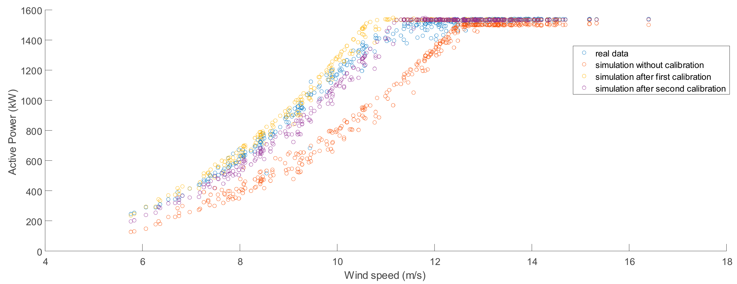
The calibration was made in two steps: in the first step, six variables were considered, while in the second step, five more variables were added.

Table 4. Design and calibrated values of parameters involved in the optimization process.

Parameters to Be Calibrated	Design Values	Calibrated Value
Stator winding resistance (pu)	0.016	0.0036
Rotor winding resistance (pu)	0.023	0.001
Generator inertia constant	0.685	0.1
Generator friction factor	0.01	0.01
Power converter grid-side coupling resistance (pu)	0.03	0.0232
Power converter grid-side coupling inductance (pu)	0.3	0.4811
Converter line filter capacitor (VAr)	120,000	89,200
DC bus voltage regulator gains	400, 8	323, 6.36
Speed regulator gains	0.6, 3	0.69, 2.67
Wind speed at nominal speed and at Cp max (m/s)	11	10
Wind turbine inertia constant (s)	4.32	2
Shaft mutual damping	1	1
Shaft spring constant	1.5	0.5

shows both the initial values defined for each parameter (design value), as well as the values adopted after second calibration (calibrated value).

The new values of the calibrated parameters are established, always keeping their physical sense. In fact, an interval with a lower and upper threshold was established for each parameter during the optimization process.

As a result, the mean absolute percentage error (MAPE) between the real active power measured in the SCADA and the value obtained in the simulation using the calibrated models improved from 15% to 2.4% (Figure 10).

3.2. Failure Hybrid Model of the Use Case

Once the physic model was calibrated, it was used to simulate the failure conditions. In this use case, the overtemperature in the stator winding was analysed. A thermal circuit was added to the already developed normality hybrid model in Simulink to estimate the temperatures in each phase of the stator winding. It must be considered that the isolation class of the stator winding is a Class F, meaning that it is designed to withstand temperatures of up to 155 °C. As shown in Figure 11, this thermal circuit takes into account heat transference generated by the stator currents considering the conduction (between the winding of each one of the three stator phases) and convection (between the winding of each one of the three stator phases, between each stator winding and the environment and between each stator winding and the rotor). The values of radiation were neglected.

Conductive heat transfer blocks model heat transfer in the thermal network by conduction through a layer of material. The rate of heat transfer is governed by Fourier’s law (18) and is proportional to the temperature difference, material thermal conductivity, area normal to the heat flow direction, and inversely proportional to the layer thickness.

$${\mathrm{Q}}_{\mathrm{cond}}=\frac{k}{s} A dT$$

(18)

Convective heat transfer blocks model heat transfer in a thermal network by convection due to fluid motion (in this case, the air). The rate of heat transfer (19) is proportional to the temperature difference, heat transfer coefficient and surface area in contact with the fluid.

$${\mathrm{Q}}_{\mathrm{conv}}=\mathrm{h}{\mathrm{c}}_{ }A dT$$

(19)

The inputs that feed the thermal model are the stator currents and the room temperature where the electric generator is installed (in this case the temperature of the nacelle), while the outputs are the temperatures of each phase of the stator winding.

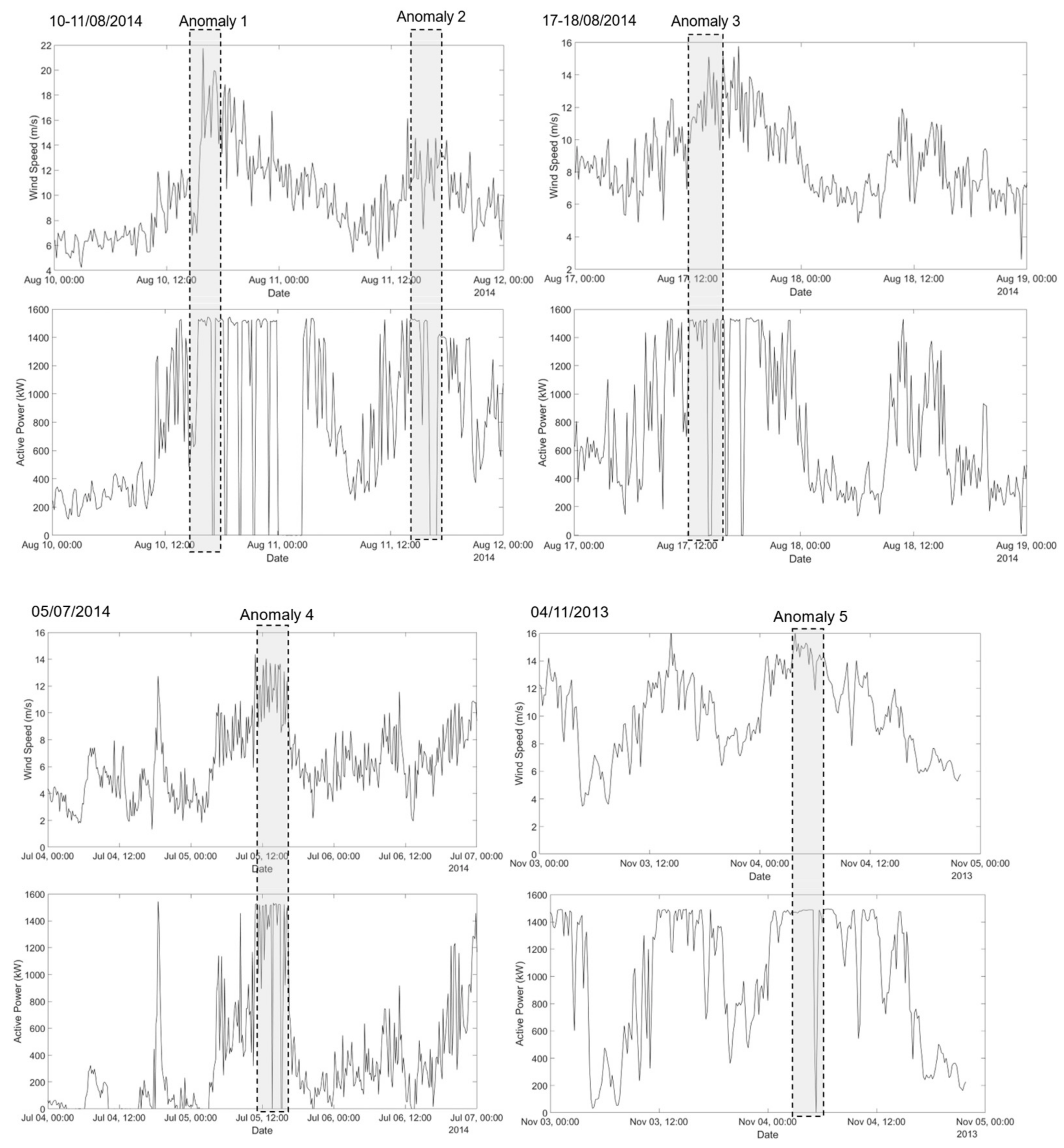
In the real data made available during this study, there are five anomaly cases labelled as overtemperature in the stator winding (Figure 12).

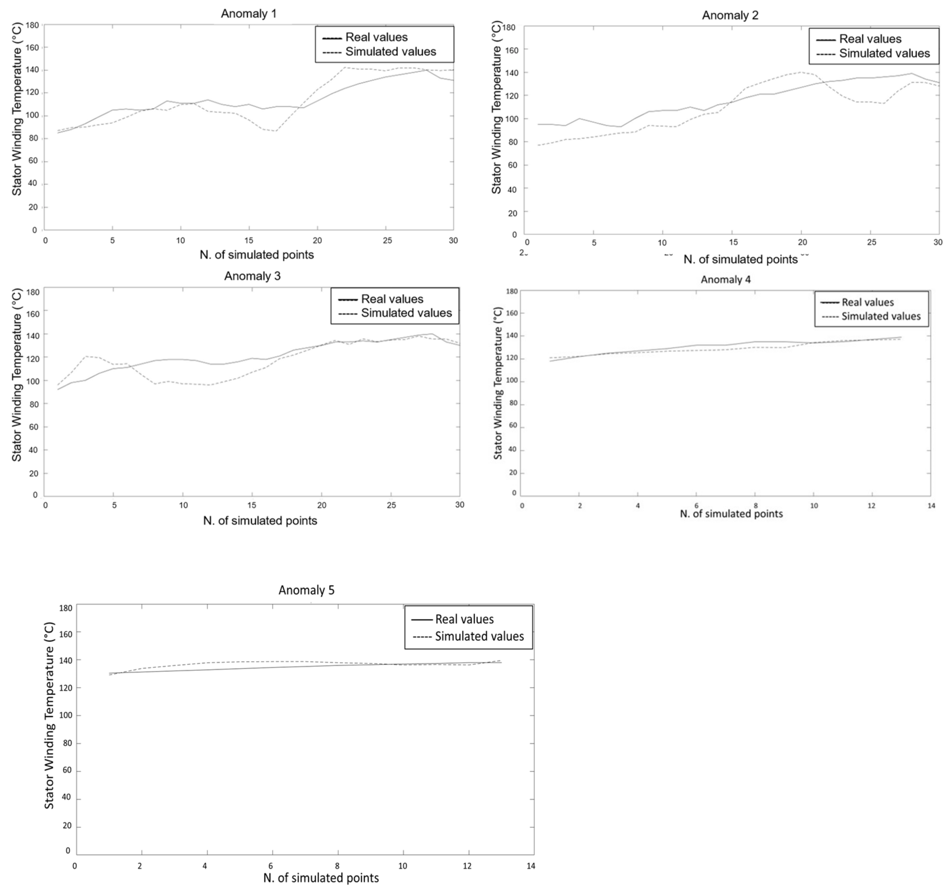
The failure modelling was validated using data during these five anomaly cases, obtaining results for the estimated stator winding temperatures, as shown in Figure 13, compared with the real SCADA winding temperature.

The MAPE between the real stator winding temperature measured in the SCADA and the value obtained in the simulation using the calibrated model has a value of 11%, with a maximum percentage error of 16% in the worst scenario. This value still has room for improvement if more accurate design data become available for the thermal model.

3.3. Synthetic Failure Data Generation in the Use Case

A failure model for stator winding overheating was trained with real data from five labelled failures. For this failure mode, four parameters (CIs) were identified: failure or anomaly duration, ambient temperature, nacelle temperature, and wind speed.

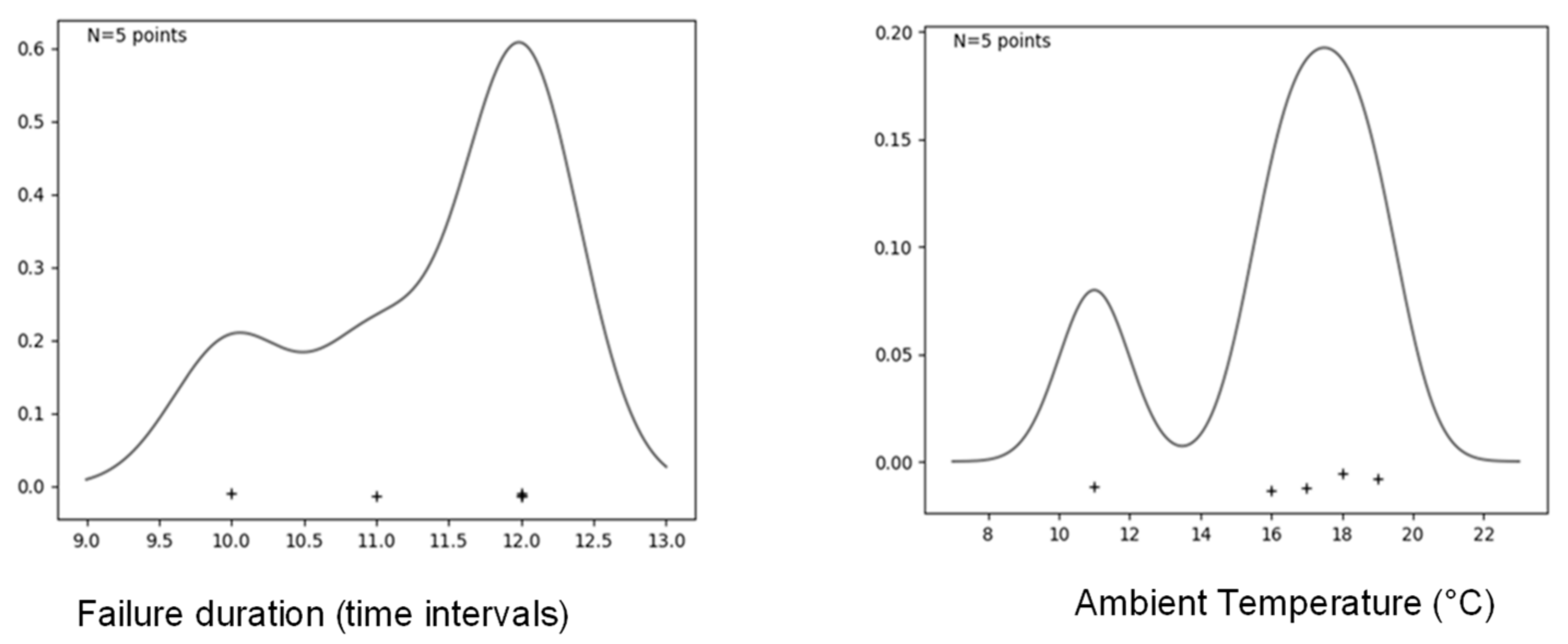
The failure duration and ambient temperature are assumed to be uniform during the whole duration of the failure. The distribution of these values in the training data is approximated with a kernel density function (KDE) with a Gaussian kernel (Figure 14). Continuous line represents the probability density functions of the duration and ambient temperature observed in the failure/anomaly instances from the real SCADA, while cross symbols represent real observations This technique, compared with density estimation by histogram, creates a smooth PDF that does not depend on the choice of binning. Instead, a Gaussian component is fitted to each data point. The Gaussian kernel is defined by the function:

$$K\left(x;h\right)\propto \exp \left(-\frac{x^2}{2h^2}\right)$$

(20)

where the density function estimated at point $x$ of a univariate distribution is:

$$\widehat{f}\left(x;h\right)=n^{-1}{{\displaystyle \sum }}_{i=1}^{n}K\left(x-x_i;h\right)$$

(21)

where $\left(x_1, x_2, \dots , x_n\right)$ are independent and identically distributed random samples from such distribution. The bandwidth $h$ is a smoothing parameter that controls the balance between variance and bias in the resulting density function. The resulting Gaussian mixture is a non-parametric estimator of the probability density function able to represent the uncertainty present in a small data sample. In addition, a domain expert can intuitively control the estimator with a bandwidth parameter based on a descriptive analysis of SCADA data and physical properties of the system.

The PDF of the wind speed and nacelle temperature variables are dependent on the relative time within a given failure or anomaly. Hence, a generative model aims to learn a PDF from which to sample a time series of a given variable, not simply a single value. Such a function can be approximated by recursively fitting an ordinary least squares (OLS) model to the transition between each time point. In this case, the resulting marginal probability distribution at a given point in time is conditional to the value at the previous time point. The statistical model of the predicted value is:

$$X_{t1}=X_{t0}\beta +\epsilon$$

(22)

Additionally, the estimation error $\epsilon$ is assumed to have a normal distribution such that:

$$\epsilon |X_{t0}~N\left(0, {\sigma }^{2}I\right)$$

(23)

where ${\sigma }^2$ is a positive common variance for the elements of the error vector (assuming homoscedasticity) and $I$ is the identity matrix.

The generation of random samples starts by the sampling an unconditional seed at time 0. This seed is randomly sampled from a distribution learnt from the training values at time 0. The distribution is approximated by KDE as seen above for the case of ambient temperature. The next data point in the time series, $X_{t1}$, is sampled from the distribution of $\epsilon$ around the prediction mean value $X_{t0}\beta$. This process iterates for each data point the requested time. Finally, synthetic failure patterns are randomly generated using the learnt statistical distributions (Figure 15) and are fed as inputs into the developed DT.

The DT generates the rest of failure synthetic measurements (e.g., stator winding temperature, and generator output current,) creating a multivariate synthetic failure scenario (Figure 16).

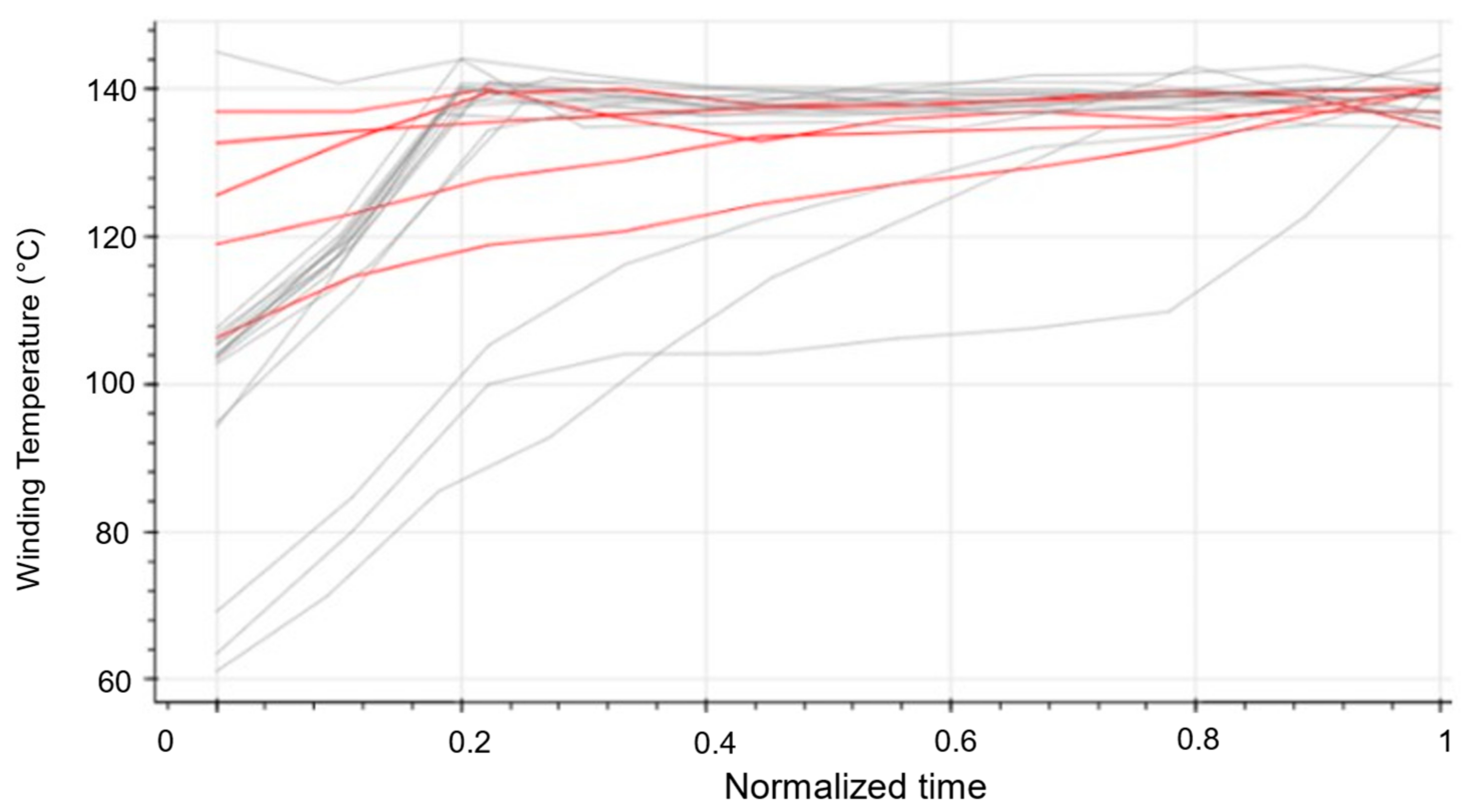
Figure 17 shows both the synthetically generated stator winding temperature values (in grey), and the stator winding real values measured by the SCADA system (in red). It can be noted that most of the synthetically generated data are similar to the real SCADA data. However, few of the synthetically generated data significantly differ from real data due to the starting seed value.

4. Conclusions and Next Steps

This paper proposes an approach for creating a hybrid model-based digital twin that combines the benefits of physics-based models with advanced data analytics techniques.

This study has two main innovation outcomes. On the one hand, a process is established to generate synthetic failure data based on real data leveraging different statistical techniques. On the other hand, the process of failure classification based on machine learning techniques, allows anomaly conditions to be identified in the operation of the wind turbine. These two innovations can provide solutions for the main limitations of current digital twin approaches regarding accuracy, explainability, and the lack of sufficient training data.

The synthetic failure data generation process was validated using real operational data from a 1.5 MW power double-fed induction generator wind farm owned by Engie. In more detail, this has been applied to a specific failure (or anomaly) mode, namely the stator winding overtemperature. The obtained results are satisfactory, although further research is necessary. One of the limitations found in current research is the difficulty in achieving detailed labelled failure information.

In future studies, the authors foresee the following research lines. It is envisaged that a developed methodology for failure diagnosis, leveraging non-supervised and supervised machine learning algorithms, could be applied, as explained in Section 2.4. The results of this research could form the basis for future publications, which will likely be derived from the methodology of this article. These algorithms will be trained using real operational data augmented with synthetic failure data generated using this methodology. Furthermore, the authors plan to assess the generalization capacity of the proposed approach, validating it with additional failure modes and other drivetrain technologies (i.e., permanent magnets). Equally, the developed hybrid models might be further improved by applying state-of-the-art deep learning techniques. Finally, the scalability of the proposed solution should be assessed by implementing and validating it in an online real-time scenario.

5. Patents

The work reported in this manuscript is associated with a patent with application number EP22382724.7.