Abstract
Most of current prosumer-energy-management approaches are focused on economic optimization by self-consumption maximization. Nevertheless, a lack of energy management strategies (EMS) that tackle different interaction possibilities among community-clustered solar plus battery prosumers has been detected. Furthermore, such active prosumer EMS may include participation in ancillary service markets such as automatic frequency restoration reserves (aFRR) through an optimized battery-energy storage-system (BESS) operation, as well as incorporating community-level energy management. In this study, an optimal EMS that includes aggregated aFRR-market participation of five solar plus battery prosumers participating in an energy community (EC), with the aim of reducing total costs of ownership for each individual prosumer is proposed. For its validation, different scenarios have been analyzed. The results show that the proposed EMS allows a levelized cost of energy (LCOE) reduction for all community members with respect to the base-case scenario. Moreover, the most profitable scenario for all prosumers is still the only PV.
1. Introduction
1.1. General Context
The climate crisis is challenging the world to reshape societies’ functioning. In this sense, one of the biggest challenges is to transform the energetic paradigm by substituting conventional and polluting energy production with innovative renewable energy sources (RES). In addition, these technologies have already been demonstrated to be reliable and cost-effective [1]. Nevertheless, many European countries continue to develop high dependency on fossil fuels.
With the aim of getting the most out of each European country’s renewable resources the European Internal Energy Market Directive (2019/944) steps towards active consumers who contribute to system flexibility, incentivizes smart grids through higher investment and information transparency and introduces a new actor in the electricity sector: the aggregator. The purpose of the aggregator is based on operating several distributed RESs in a coordinated manner, creating a sizeable capacity similar to a conventional generator (microgrid or virtual power plant) with the aim of acting as a unique entity or market unit in wholesale, retail or ancillary service markets and, therefore, contributing to the system’s flexibility [2]. This new agent manages different figures so that they get the capability of intervention in electricity markets: daily market (DM) and continuous intraday market (CIM) as well as, ancillary service (AS) markets such as the automatic frequency restoration reserve (AFRR) and, therefore additional benefits that could not have been obtained individually can be achieved. Likewise, given its versatility it is likely to become a highly promising business in the near future.
Regarding the Spanish case, the Spanish Royal Decree 244/2019 replaced RD 15/2018, which exposed urgent measurements for energy transition. This new measure allows self-consumption activity. Therefore, consumers will be able to produce their own electricity and even sell their surpluses, becoming prosumers. These alternatives can be individual or shared through an internal grid, and surpluses or deficits can be poured in the LV distribution grid. Further, the constant cost reductions that come with the technology improvement makes even more attractive complementing household photovoltaic (PV) generators with battery-storage devices. This binomial enables solar energy consumption whenever it is needed and, therefore, can improve overall efficiency by maximizing autarky and minimizing technical constraints.
A RES plusbattery scheme represents an enabler tool to maintain the balance. On the other hand, the role of the aggregator is managing distributed prosumers’ facilities in exchange of providing them a saving, as well as perceiving a revenue because of offering ancillary services to the transmission system operator (TSO). Therefore, optimum energy-storage-management techniques provide the flexibility needed and will benefit the rest of the stakeholders.
As has been indicated, all these distributed resources can be clustered in configurations such as microgrids (MG) or virtual power plants (VPP). In order to differentiate them, some features can be highlighted [3]: by definition, a VPP is a cluster of distributed generation facilities that have the capacity of intervening in energy and ancillary markets due to resource aggregation. VPPs are grid-tied, do not require storage (economic advantage) and rely more on communications. On the other hand, microgrids consist of distinct hardware such as protections or inverters. In addition, while most microgrids cover a limited area with complex algorithms, VPPs are geographically spread and require simpler algorithms. Nevertheless, there exists a main reason that makes VPPs more suitable for pooling processes: not having to face legal and administrative hurdles. Therefore, this solution can be much more easily implemented in existing legal and technical frameworks.
EMSs play a crucial role when offering flexibile services since these enable the optimal schedule, operation and dispatch of a DER-based portfolio. That is why the following section focuses on existing EMSs and provides, consequently, a review of those applied to microgrid and VPP applications.
1.2. Energy Management Strategies for Microgrids and VPPs
Regarding MGs, diverse EMSs with different objectives have been reported in the literature. Most of them can be classified in terms of the associated benefits they aim to achieve which can be technical, economic, environmental and social (mainly techno-economic and economic–environmental). Remarkably, EMSs can also be categorized by the DERs involved and/or the utility grid–energy-market interaction, most of them being focused on economic optimization.
From the techno-economic point of view, objectives such as load-peak shaving, voltage regulation, energy-loss minimization (or energy-efficiency maximization) and/or reliability enhancement can be set. Most of them are mixed with economical optimization objectives such as lowest levelized cost of energy (LCOE) obtainment or minimization of grid intake for enhanced revenue. For instance, in [4] Ramli et al. proposed a multi-objective self-adaptative differential evolution algorithm (MOSaDE) for cost minimization, RES share maximization and lost power-supply-probability optimization. This EMS was evaluated in the Saudi Arabian framework considering PV, wind turbine (WT), BESS and diesel generators’ contributions. In [5], a multi-agent system for a MG real-time operation was developed achieving DER-production maximization, operational cost reduction and MG–utility grid power-exchange optimization. The proposal is a two-stage scheduling (day-ahead and real-time) strategy for PV panels, a fuel cell, distributed generators and a battery bank which considers demand-side management (DSM) and suggests a common communication interface (IEEE FIPA) for these devices. The EMS was validated in a real-time digital simulator.
Pursuing MG management in energy markets, in [6], the authors propose a MG centralized control technique that considers economic scheduling, load-generation forecasting, security assessment and DSM functions. The strategy bids in 15 min intervals and minimizes energy costs by central-load-microsource–controller interaction taking into account market prices, DERSs’ bids, demand-side bidding and production limits. In [7] a day-ahead scheduling strategy was developed for wholesale and ancillary market participation. Several ASs are provided by applying a robust optimization approach within the PV, WT, BESS and combined heat and power-based system (CHP-based system). Maleki et al. report in [8] a particle swarm optimization Monte Carlo-based algorithm for a PV, wind turbine and battery-based MG in Iran. The strategy attempted to find the optimum number and sizing of generation–storage units while dealing with uncertainties and optimizing the total costs for different times of the year (i.e., different RES share).
Several studies propose optimization algorithms for optimal sizing of hybrid source-based MGs in a standalone framework. In [9] the system reliability was analysed in terms of loss of energy and load expectations for a PV, WT, fuel cell and battery bank-based system. Aside, an economic optimization analysis was conducted for different locations, times of the year and RES-share degrees in Iran. A similar sizing optimization study was reported in [10]. In this case, an artificial bee-swarm-optimization algorithm has been proposed for total annual cost and loss of power-supply minimization.
Economic–environmental EMSs are also widely studied in the literature. Within these, CO2 emissions or physical footprint minimization stand out. Maximizing RES share can be seen as a doubly beneficial goal because it maximizes revenues while reducing emissions. In [11] Di Somma et al. applied a stochastic multi-objective linear programming technique for total daily energy cost and CO2-emissions minimization in a PV, BESS, heat pump and CHP system-based environment. A similar study was carried out by Rezvani et al. [12]. In [13] and [14] CO2 and LCOE-minimization objectives were pursued simultaneously. Nevertheless, while in [13] a genetic algorithm was used for a RES and conventional source-based system, in [10] historical data-based optimization was developed in rural and urban MGs in India. Aluisio et al. reported in [15] an optimization procedure for day-ahead scheduling in a PV, WT, BESS and CHP-based MG aiming to minimize operation and emission costs. These four methods have been tested using SCADA/EMS hierarchical and Modbus communication-network systems. In this sense, in [16] a techno-economic analysis of a solar-PV and DC battery storage system for a community energy sharing is implemented.
In [17] the coordination of VPPs with the system operators and their commercial integration in the electricity markets was analysed. In [18,19] an integrated model to undertake a multi-disciplinary assessment of a potential EC was proposed. Fonseca et al. [20], contributed to the management and optimization of individual and community DER following a price and source-based EC-management program, in which consumer’s day-ahead flexible loads were shifted according to electricity-generation availability, prices, and personal preferences, to balance the grid and incentivize user participation. In this sense, in [21] a novel decentralized energy-scheduling framework for demand response on energy communities in the case of limited overall capacity of distribution networks was presented. Hosseini, in [22], proposed a framework for the day-ahead energy scheduling of a residential microgrid. Moreover, users shared a number of RESs and an energy-storage system. The author assumed that the microgrid could buy/sell energy from/to the grid. The objective of scheduling is minimizing the expected energy cost while satisfying device/comfort/contractual constraints, including feasibility constraints on energy transfer between users and the grid under RES generation and user-demand uncertainties.
1.3. Identified Gaps
A major part of the literature related to MG EMSs is focused on economic optimization techniques. In terms of energy resources, a wide range of technologies are implemented for enhanced MG resiliency and/or RES share maximization, leading therefore to minimum operational and emission costs. Regarding market participation, as far as it has been evaluated, day-ahead scheduling for wholesale market intervention has been found to be the most abundant research topic. Fewer studies tackle AS market intervention and the ones that do are mostly focused on spinning reserve supply through distributed generators (i.e., gas or diesel engines). None of the studies analysed considered BESS ageing because most of them use storage devices for backup power instead of for selling AS. Likewise, no virtual microgrid (VMG)-management strategy has been found, i.e., all configurations considered customer or remote MGs where all components were connected downstream of the point of common coupling (PCC).
Therefore, after reviewing the literature related to the research topic, the lack of a PV plus BESS residential prosumer-focused EMS has been identified. Moreover, a need for strategies for configurations that include aFRR-market participation through a BESS-optimized operation that reduces total energy costs has been identified. Even though this type of configuration limits MG management in terms of resiliency and sufficiency, it has been regarded as an attractive alternative due to the recent self-consumption incentives and the possibility of building a community-based and cost-effective approach. Therefore, considering a fully deterministic model where the aggregation strategy uses historical data has been found to be a focus of interest in order to obtain the most accurate results possible in a given scenario, even if real-time operation involves uncertainties in demand, generation and price signals. Thus, one of the first steps of this work has been to build a preliminary accurate management model so in further steps it can lead to the implementation of optimization tools that would deal with such uncertainties.
In summary, the main contributions of this paper are:
- Introduce concepts about ECs, their scope and limitations and evaluate the benefits offered by EC in different scenarios;
- Propose an algorithm that tackles EC management and its later participation in electricity markets;
- Develop an optimal EMS that includes aggregated aFRR-market participation of five solar plus battery prosumers participating in an energy community (EC), with the aim of reducing total costs of ownership of each individual prosumer is proposed;
- Create a scalable and modifiable algorithm that allows analyzing the different self-consumption configurations legislated in the Spanish RD 244/2019. The developed tool can study all these by switching on/off the community mode, the BESS and/or PV production;
- Design a tool that allows the identification of the main drivers that would make the strategy proposed by the EMS profitable for each type of prosumer, analyzing different scenarios.
To reach that goal this paper is structured as follows: in Section 2, the proposed methodology and used equations are described and an analysed use-case is presented; Section 3 focuses on detailing the obtained results and the comparative analysis between scenarios; lastly, in Section 4, the most remarkable conclusions and future research lines are presented.
2. Methodology
This section’s aim is to expose the developed strategy for solar plus battery-based VMG management within the Spanish framework as case of study. As mentioned before, the main goal of the project was to develop an EMS that benefits both system operators and end-users by providing frequency stabilization while reducing prosumers’ annual electricity costs.
Thus, first a contextualization of the strategy is provided. Second, a general overview and the scope of the strategy are discussed. Next, the study case is described in detail, enabling a later understanding of the VPP operation. In a further step, DM and CIM participation principles are discussed. Finally, a summary of the proposed technique is provided.
2.1. Contextualization
This work proposes an algorithm that tackles EC management and its later participation in electricity markets. In this sense, the algorithm consists of several hierarchically structured layers that communicate with each other. The hierarchy of the EC is composed of three main levels of energy management. First, a household or home-scale scheduling is carried out. Then, community-level management is obtained by adjusting their deficits/surpluses with the aim of maximizing the overall self-consumption level. Finally, once adjusted, the community as a MG, is pooled in energy markets as a VPP or single entity by a virtual aggregator.
That results in an algorithm that operates through two-stage scheduling: a day-ahead planning and a real-time re-scheduling (see Figure 1).
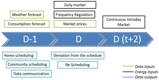
Figure 1.
Two-stage scheduling of the energy community.
2.2. General Overview and Scope
The MG-management strategy comprises the first two management levels of the hierarchy (home and community). In the first level, the individual household self-consumption maximization is pursued by controlling BESS charge and discharge cycles depending on the relationship between solar production and consumption. In this level, power flows through the smart meter are controlled to avoid outages and maintain compatibility. Once all prosumers have been individually managed, community-level scheduling is developed. In this level, the main goal is the same, maximizing PV plusBESS energy consumption but under an EC vision, i.e., when prosumers’ deficits and surpluses exist within the same hour, these are matched and excess/lacking energy is bid in the DM. If not, the state of charge (SoC) of each prosumer is checked in order to take advantage of or cover any member’s excess or needed energy. If all SoCs are within the operating limits, no bids will be sent; or if, conversely, no exchanges can be scheduled, the excess or lacking energy will be sent as an offer to the operator the day ahead.
Nevertheless, the DM offers sent to the market operator are not definitive because FRR market participation modifies individual SoCs. Therefore, CIM intervention is usually required for two main reasons: to correct the DM bid sent the day before, maintain a secure SoC, and optimize expenses of all prosumers by trading and doing energy arbitrage. This second CIM intervention is part of the strategies developed by the VPP operator. For an optimized real-time operation, information flow between community manager and VPP operator is crucial; therefore, in Section 2.4, the data exchange is detailed.
Regarding the scope of the methodology, it is divided into two main objectives:
- To obtain extra monthly savings in the electricity bill by aggregating prosumers and offering aFRR services to the TSO. For that aim, as mentioned, optimized energy trading techniques have also been implemented for enhanced operation and revenue maximization;
- To analyse future scenarios for energy consumers in economic terms within 15 years after evaluating the profitability of the EMS on a year basis. These scenarios are: (1) utility grid consumption or business as usual (BaU); (2) installing only PV panels and participating in the net billing scheme developed recently; (3) adding a BESS to the net billing scheme; and (4) joining an energy community based on the proposed EMS. The developed tool can study all these by switching on/off the community mode, the BESS and/or PV production.
2.3. Definition of the Case of Study’s Scenario
The energy-community object of study is composed of five prosumers who have different consumption profiles among them. Remarkably, all the input data was obtained from real data sources for the November 2021 to November 2022 period. Among these, solar irradiance information was obtained from the weather agency’s website [23] and from the closest weather station to each prosumer, and energy consumption data were obtained from real metering data reported on their distribution-company application [24].
After obtaining the consumption data for each user, the PV and BESSs were sized, and solar production was calculated following common criteria. Solar arrays’ configuration was designed following the solar peak hours (SPH) criterion aiming to obtain an annual solar coverage ratio (SCR) of 100%. Briefly, with this criterion the equivalent hours of maximum daily irradiance (SPH) were obtained with historical hourly irradiance (Gmaxday) data by using Equation (1). Afterwards, the amount of required solar panels was calculated with Equation (2) using yearly mean SPH obtained in 2.1. Finally, monthly mean SCR was calculated using Equation (3):
with Gmeanday being the mean hourly solar irradiance [W/m2], hday the 24 h per day [h], Gmaxday which was considered 1000 [W/m2], nPV the number of PV panels [−], PPV the power of the panel [kW] which was considered 0.3 kW each, ηsyst the efficiency of all the systems [pu] which was considered 90% (i.e., 10% conduction and module losses), SPHmean yearly mean SPHs [h], SPHmonth monthly mean SPHs [h] and Econ_meanday the mean daily consumption of a given household.
SPH = (Gmeanday·hday)/Gmaxday,
nPV = (Econ_meanday PPV·ηsyst)/SPHmean,
SCR = (nPV·PPV·ηsyst·SPHmonth)/Econ_meanday,
The annual PV production has been calculated using Equation (4):
with Etotalyear being the total annual solar irradiance [kW·h/m2], ηpanel the efficiency of each PV panel which was considered 18.2% [pu], Spanel the surface of each PV panel which was considered 1.6 [m2] and nPV the number of PV panels resulting from Equation (2).
EPV_year = (Etotalyear·ηpanel·Spanel·nPV),
For BESS capacity (Ebat) sizing, taking into account self-consumption maximization and aFRR requirement premises, Equation (5) was applied:
with Econ_meanday being the mean daily consumption of a given household, aut the autonomy required for the battery [fraction of daily hours] (i.e., 0.25 for 6 h) and DoD expected daily depth of discharge [pu].
Ebat = (Econ_meanday aut)/DoD,
All data comprising market values were extracted from the Spanish transmission system operator (TSO) database [25], i.e., pool prices, regulated prices, aFRR bands and aFRR prices. Because the data are provided in hour periods, this information was directly included in the algorithm.
In addition, device costs were obtained from a local RES-facility installer for a higher accuracy considering workforce, additional components, the VAT and government grants for the given year.
Table 1 shows the resulting data for each facility once they were sized and each’s PV production was calculated. The given values refer to each location, weather station, contracted power, solar and storage capacities, annual consumption and resulting annual PV production.

Table 1.
Resulting data of user’s self-consumption facilities.
2.4. Home, Community and VPP Operation
After scheduling each self-consumption facility on an hourly basis, an aggregated or community-level planning was carried out considering the results obtained in the lower level. Finally, once the whole community was managed the day before, an upper-level management was developed by the VPP operator. Apart from adjusting the deviations between the day-ahead planning (D-1) and real-time operation (D) derived from aFRR-market participation, some strategies were also set during operation in order to maintain SoC within secure values and maximize the revenue for grouping. Remarkably, home and community algorithms were not just performed in D-1 but also in D for re-scheduling 2 h before operating the aggregated plant. Regarding algorithm time horizon, it was run continuously for a whole year, hour by hour.
At the foundation level, a device-level EMS based on the hourly difference (Edif) between PV production (EPV) and consumption (Econ) inputs was developed. The proposed algorithm will charge or discharge each battery (being Ebat the capacity in kW·h), considering the efficiency (eff_bat = 90% for both processes) and depending on the current SoC (home SoC) and the value of Edif each hour. Therefore, a negative value means discharging the battery and a positive (PV > consumption) the charge. Equations (6) and (7) show how the battery is discharged or charged, respectively, for updating the SoC for the next time-step (t + 1), i.e., the beginning of the next hour:
SoC (i, t + 1) = SoC (i, t) + ((Edif (i,t)/eff_bat)/Ebat (i))·100,
SoC (i, t + 1) = SoC (i, t) + ((Edif (i,t)·eff_bat)/Ebat (i))·100.
It is important to remark that the upper and lower SoC limits are set in 85% (maximum SoC, SoCmax) and 15% (minimum SoC, SoClim), respectively, in order to maintain the available frequency band (10% up and 10% down). SoC security limits, which aim to avoid severe cycling, are set in 95 and 5%. When SoC limits are reached or will be reached during that time-step, the algorithm generates a variable named Eint that represents the interchangeable energy between community members and/or market. This variable stores the difference between the energy that needs to be discharged from (Equation (8)) or charged in (Equation (9)) the battery and the available energy or storage capacity for each time-step. When the lower limits are reached, Eint has a negative value and, conversely, when no storage is available, excess energy is saved as positive. If the battery has already reached limits, all the energy (Edif) will need to be imported/exported (Equation (10)). On the contrary, if batteries can stand the demand, that time-step, Eint will be zero. The calculations are carried out as follows:
and
where Eav represents the available energy in each BESS for each time-step. Its upper (Eav_max) and lower (Eav_min) limits are SoC limits in energy values. Through this, the interchangeable energy is calculated by using the presented equations. Hence, this level calculates the hourly SoCs and Eint, which are the inputs at the community level. Reaching this point, no energy has been auctioned yet as a DM offer (Emkt_DM), because it is still necessary to evaluate the system at the community level, i.e., to check if energy sharing is possible. In order to have a better understanding of the operation of the home-level algorithm, its flux diagram is shown in the Figure 2.
Eint (i, t) = Edif (i,t) + (Eav (i,t) − Eav_min(i))·eff_bat,
Eint (i, t) = Edif (i,t) − (Eav_max(i) − Eav (i,t))/eff_bat,
Eint (i, t) = Edif (i,t),
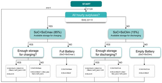
Figure 2.
Home-level algorithm’s diagram flux.
Once individual scheduling has been carried out, collective planning starts. This management level takes some of the outputs from the level below as inputs. For instance, SoChome, which becomes SoCcommunity, and the interchangeable energy (Eint: Eexp[+] and Eimp[−]) of each prosumer for each time-step. Once it knows these parameters, the EMS aims to maximize the overall self-consumption ratio by adjusting the existing surpluses–deficits and/or by balancing individual SoCs through different techniques. The results of this community-EMS-level the day ahead are market bidding offers for each hour of the day and, as known, the forecast is considered successful because fixed historical data have been used (a more accurate strategy would need to consider these parameters under a level of uncertainty). Figure 3 shows the simplified diagram flux of the community-level algorithm.
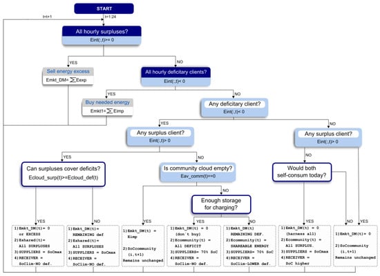
Figure 3.
Simplified community-level algorithm’s diagram flux.
In this community-level algorithm, three alternatives for energy exchangre have been implemented, which are checked in sequential order:
- First check If in a given time-step all prosumers have deficits or surpluses, then all that energy will be needed to be bought or sold. Therefore, the sum of Eimp/exp will be the bid offer that hour to the DM (Equations (11) and (12)). Typically, this may happen during night hours when the battery is fully discharged and energy demand exists or, conversely, during sunny hours with low consumption and fully charged BESS.Emkt_DM (t) = ∑Eimp (i, t)Emkt_DM (t) = ∑Eexp (i, t).
- Second check If in a given time-step there are prosumers with energy deficit and surplus, then the excess (Ecloud_surp) and deficit (Ecloud_def) energy would be stored in the cloud, as shown in Equations (13) and (14), for a later proportional share (Eshared). The shared energy would depend on the amount of energy stored in both clouds so, as shown in Figure 3, if surpluses exceed deficits, all individual surpluses will be shared and, conversely, if deficits exceed surpluses, all these will be given to users with an energy deficit; i.e., Eshared will be Eexp or Eimp, respectively. In case surpluses and deficits do not match, an equitable share will be programmed as shown in Equations (15) and (16). By these, it is aimed to maximize the overall self-consumption ratio while promoting fair participation. This energy sharing is conducted through the existing utility grid and, therefore, the corresponding energy-access toll per each power unit will need to be paid. When the hourly surplus is higher or lower than the existing deficits, the difference between these is saved and individualized as Esurp lor Edef, respectively, as shown in Equations (17) and (18). These parameters are converted to Esurp_comm (remaining surplus energy) and Eneed_comm (remaining deficit energy), which are the ones that are checked for a third time before sending the definitive offer to the DM (Emkt_DM). Typically, this may happen during mid-day hours when consumption patterns among prosumers differ a lot.Ecloud_surp (t) = ∑Eexp (i, t)Ecloud_def (t) = ∑Eimp (i, t)Eshared (i,t) = (Eexp (i, t)/Ecloud_surp (t))·Ecloud_def (t)Eshared (i,t) = (Eimp (i, t)/Ecloud_def (t))·Ecloud_surp (t)Esurp (t) = Eexp (i, t) − Eshared (i, t)Edef (t) = Eimp (i, t) − Eshared (i, t).
- Third check. If in a defined time-step prosumers with energy deficit/surplus or high/low SoC exist, the battery will discharge to cover deficits or charge batteries. In the first case, if any prosumer’s SoC is between 70–85% and its demand is expected to be covered during the day (to avoid purchasing during expensive hours), then this will make available (Eav_comm) its battery to discharge up to 70% so as to cover totally or partially others’ deficits (Eneed_comm), as shown in Equations (19) and (20). Then, in the same manner as the second check, proportional sharing is programmed (Ecommunity) and remaining hourly deficits are bid to the DM as shown in Equations (21) and (22), respectively. Conversely, if any prosumer’s SoC is between 15 and 30% and others still have surpluses, as long as both are expected to cover their demand during that day, this will charge the battery until all hourly surpluses are harnessed (see Equation (23)). In this case, no market bid would be sent because all surpluses would have been utilized and there would be no energy deficit. Therefore, the only expense corresponds to the shared energy. In this case, the energy sharing is conducted through the existing grid, which requires that tolls be paid.
SOC (i, t + 1:end) = SOC (i, t + 1:end) + (SOC (i, t + 1) − 70)
SOC (i, t + 1:end) = SOC(i,t + 1:end) + (Eneed_comm(t)/Eav_comm)·(SOC (i, t + 1) − 70)
Ecommunity (i, t) = ((Eneed_comm(t)/Eav_comm(t))·Efalta (i,t)
Emkt_DM (t) = Esurp_comm − Echarge_comm
SOC (i, t + 1:end) = SOC(i,t + 1:end) + (30·Esurp_comm(t)/Echarge_comm) − (SOC(i, t + 1))
Ecommunity (i, t)= ((Esurp_comm(t)/Echarge_comm(t))·(30 − SOC (i,t))·Ebat (i)
Once all of the community has been managed, the corresponding hourly DM offers would be sent to the market operator. At this point the energy purchase is programmed in order to minimize grid-intake expenses. Hence, the DM scheduling only seeks to offer uninterrupted supply by adjusting the community. In fact, this trading optimization, which can be regarded as energy arbitrage, is carried out by the VPP operator by means of different strategies that are presented in Section 2.5. As to variable communication with the VPP operator, the ones transferred are the updated SoCs (SOCcommunity) and hourly bids (Emkt_DM) the day before and the global SoC of the operation day (globalSOCreal), which is the weighted average of the individuals (SOCcommunityactualizado) once re-scheduled in the community on a real-time basis (see Figure 4).
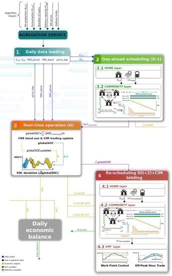
Figure 4.
Simplified methodology of the EMS, which comprises MG and VPP controls.
The role of VPP operators is to balance the community operating in the target markets. Therefore, his two main tasks consist of dealing with the imbalances caused by FRR markets in the day-ahead scheduling and maximizing the economic revenue of his portfolio during operation.
Deviations occur because FRR participation hourly modifies the SoC of the batteries by increasing it when regulation is downwards (energy absorbed from the grid because production > demand) and decreasing it when regulation is upwards (energy poured into the grid because production < demand). In addition, energy arbitrage for SoC control and off-peak-hour purchase strategies have been implemented. Figure 4 shows the simplified step-by-step methodology.
Hence, after describing the developed methodology, the following section focuses on explaining in detail the DM participation of the community. This comprises bidding proceedings and the followed sequence in order to contextualize CIM adjusting.
2.5. Daily Market Participation
The day-ahead or DM participation consists of each hourly bid sent to OMIE the day before operation.
After, the preliminary plan is sent to the TSO for a verification of its technical viability. All bids must be sent before 12 h, so real-time operation of that day and the scheduling for the following one happen at the same time. This fact implies uncertainty because all factors that modify real-time state will affect the oncoming day, i.e., it is complex to send an accurate DM bid because there are still twelve hours left of operation that are susceptible to modifying the SoC with which prosumers will start the next day. To comply with market-gate closure, it is considered that all prosumers start the following day with 35% of SoC. The deviation must be corrected by the VPP operator in the CIM so that all values stay within limits when operating. Therefore, real-time operation would be the sum of the day-ahead planning and CIM re-scheduling. At the day start-up, an initial SoC of 50% is considered and the schedule for that day is identified as correct because no day-ahead planning exists then. Figure 5 shows the timeline of this process:
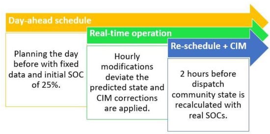
Figure 5.
DM bidding and real-time superposition timeline.
2.6. Continuous Intraday Market Participation
CIM intervention consists of sending a bid hourly to the market during the operation day with a margin of two hours. Several factors intervene in such offers in this case study. For instance, FRR SoC deviations, schedule adjustments derived from the aforementioned and optimization strategies implemented by the VPP operator.
FRR or secondary reserve services every hour modify global and, therefore, individual SoC curves; this is the reason why re-scheduling is necessary at the community level. A 10% up−10% down frequency band is reserved for such services so individual limits already consider this requirement. The requested percentage of the frequency band and the retribution perceived are fixed data but are entered as unknown in the algorithm, i.e., these parameters just affect during operation as in reality no anticipation is possible. Therefore, this level of the proposed algorithm is divided into two processes, the re-scheduling and the optimization:
- The re-scheduling process is based on operation-day planning with real SoC values. At this point, the current SoC of all batteries is already known and, therefore, it is possible to schedule more accurately, at least for the oncoming two hours, having just as uncertainty frequency-service deviations of the next two. Through this process real deficit/surplus and exchanges are estimated and communicated to the VPP operator so that they correct DM offers in the CIM and the final plan complies with all requirements.
- Optimization strategies aim to maximize the profitability. Two main strategies can be distinguished:
- Off-peak hour trading (OPT): its goal is to purchase energy during the cheapest hours of the day so that prosumers dispose of a SoC close to 55% by the time they start consuming (6–7 am approximately). Thanks to this, severe energy purchasing during more expensive hours is avoided.
- Work point control (WPC): its main objective is to maintain the SoC of the community within its limits by trading in the CIM. Apart from it, this strategy also considers market prices within two hours and seeks to optimize the trading depending on the existing price, i.e., the control maintains a secure SoC while conducting energy arbitrage. For instance, if batteries are close to upper limits, these will discharge more or less energy depending on the price. The opposite would happen if lower limits were about to be reached. Figure 6 depicts the selected limits for the WPC strategy:
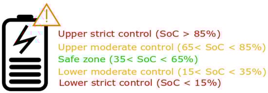 Figure 6. WPC strategy’s limits.
Hence, the developed EMS comprises a community scheduling into a VPP configuration whose timeline goes from the day-ahead planning (D-1) to a real-time operation (D) that can effectively work thanks to CIM anticipation (Dt + 2). DM offers added to CIM adjustments and strategies represent the final bids, which are later translated to a daily economic balance. Finally, a definitive hourly SoC value is obtained. Figure 7 summarizes the variable communication between stages:
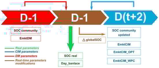
Figure 7.
Variable communication between EMS stages.
3. Results
This section focuses on explaining all the results obtained from the several simulations that were carried out. This section consists of five main axes: first, the bases and the equations applied in the four study cases and the electricity-market assessment derived from the EMS are exposed; then, the investment costs of each prosumer are given; afterwards, the obtained results of the study cases and the market assessment are provided and; later on, a sensitivity analysis is carried out so as to identify the most relevant parameters and their influence. Finally, the discussion and the summary is tackled.
3.1. Cases of Study
In this section, the cases of study that have been analysed with the EMS are presented. Four scenarios (A, B, C and D) presented in Table 2 are considered to analyse the viability of the proposed business model, compared with other options that the consumer can adopt.
Table 2.
Definition of the analysed scenarios.
The viability is analysed on a 15-year basis. It is assumed that no replacement of the BESS will be needed because of moderate use during this period. Likewise, no changes in market prices over the 15 years has been considered.
Applied Equation(s)
In the present section the applied equations for the economic analysis and the difference between the selected parameters of each study case are presented. A single equation has been implemented to evaluate the four study cases. Just modifying input parameters and using the same equation was found to be a more comprehensive solution compared to individualized calculations. Equation (25) was used to calculate the economic profitability of each study case:
where the involved parameters in the equation are those defined in Table 3:
Cost15years = 15·(TP·Pinst·364 + ((((−Ebuy·(PVPC) +TE·Ecomm − (EmktCIM_deficit + EmktCIM_strategies_deficit)·PVPC_CIM_deficit) − (Esell·PVPCautoconsumo + (EmktCIM_surplus + EmktCIM_strategies_surplus)·PVPC_CIM_surplus))·Elec_TAX) + others·364)·IVA + panel_price·PPV + workforce_pv + price_bat + workforce_bat − (15·year_balance_r2),
Table 3.
Breakdown of the parameters in Equation (25).
3.2. Electricity Market Assesment
In the present section, the electricity-market assessment resulting from the proposed EMS is presented.
The proposed EMS seeks to offer economic savings to facility owners while providing them uninterrupted RES-based supply. Therefore, obtaining an annual balance lower than study scenario A, i.e., consuming from the utility grid, would be the indicator that represents the effectiveness of the proposed strategy. The perceived savings quantity, which is proportional to the size of the installation, would be translated into a lower payback for facility owners and could make investing in BESSs profitable; i.e., could make the community study case the most interesting. However, the annual economic profitability is the result of optimizing the management method by proper community planning and market participation, a fact that is not ensured until simulating. Study cases depend on a lot of other factors such as device costs or tariff-structure modifications.
The following section presents the equations that were applied for calculating the economic balance result from energy-market intervention. It divides this balance into different concepts and explains how annual energy costs were consequently reduced or increased.
Applied Equations
Annual results are the sum of daily economic balances and are individualized for each prosumer. Furthermore, daily balances are compounds of different concepts, for instance, energy and ancillary service market results. Regarding energy markets, two main sources must be distinguished: energy trading for uninterrupted supply and optimization strategies. The first corresponds to the definitive bids, which are the sum of day-ahead offers and intraday corrections, i.e., prosumers’ needs. As to optimization techniques, these comprise the WPC of the global SoC and the OPT strategy implemented to take advantage of the cheapest prices. Yearly economic balance was calculated as the accumulation of daily market interventions (d = 1:364); both parameters are measured in euros:
Year_balance = ∑Day_balance
Daily economic balance [EUR] is determined by hourly (t = 1:24) market participation (balance_mkt), community exchanges (balance_comm) and frequency of service offering (balance_r2) results as shown in Equation (27):
with balance_mkt being market intervention balance [EUR], balance_comm the daily community exchange expenses [EUR], balance_r2 balance obtained from FRR services [EUR], revenue_mkt [EUR] and expenses_mkt [EUR] the daily earnings and expenses, respectively.
Day_balance = balance_mkt + balance_comm + balance_r2,
balance_mkt = ∑revenue_mkt + ∑expenses_mkt,
Daily earnings (+) and expenses (−) that appear in Equation (28) represent the economic translation of the sum of hourly traded energy. Energy prices that must be applied vary depending on the market that was traded in. For instance, energy traded in CIMs (bid adjustments, WPC and OPT all together) are attached to different prices in comparison to DM energy bids. Equations (29) and (30) show how earnings and expenses were calculated, respectively:
and
Revenue_mkt = (Emkt_DM + Emkt_CIM)·price_day,
Expenses_mkt = gastos_mkt_DM + gastos_mkt_CIM.
As previously mentioned, DM and CIM energy fluxes perceive different prices, that is why Equation (30) distinguishes expenses into two concepts: the prices considered are the regulated tariff or PVPC for DM bidding and 105% of PVPC for CIM, respectively, as shown in Equations (31) and (32). The PVPC has been considered because of the aggregator-supplier model has been assumed so all regulated costs have to be considered, in consequence. Nevertheless, earnings due to exported energy are all retributed applying whole market prices.
and
where the regulated tariff is translated to EUR/W·h and energy fluxes in W·h.
Expenses_mkt_DM = Emkt_DM·PVPC
Expenses_mkt_CIM = Emkt_CIM·PVPC·1.05,
Regarding aFRR-service economic balance, this is composed of an energy and a power term. Thus, the provided energy is a function of the demanded percentage of the offered available band. In this case the band is 10% up and 10% down of each battery. The balance is calculated as shown in Equation (33):
with Euso_up and Euso_down being the used (required % offered energy) upwards and downwards energy [W·h], respectively, price_r2up and price_r2down the price signals for up and down [EUR/W·h], respectively; Pband_up and Pband_down the offered power bands [W] and price_band the price signal for such available band [EUR/W].
balance_r2 = (Euso_up·price_r2up) + (Euso_down·price_r2down) + (Pband_up + Pband_down)·price_band,
Once the annual economic balance is obtained, contracted power costs and taxes are added in order to estimate the total energy costs. These are calculated individually as function of each contribution as shown in Equation (34):
Individual_year_balance = (abs(year_balance)·(Ebat/globalcapacity) + (TP·Pinst·364))·Elec_TAX·IVA.
The percentual variation of them is the economic success indicator of the proposed EMS.
3.3. Facility Invesment Costs
Investment costs have a crucial impact in the study case economic analysis but are applied in the first year. Therefore, all costs have been considered for the given year. These costs comprise several expenses, not just hardware. For instance, the workshop for each technology, which includes cables and protections, additional components such as structures for PV panels, VAT and economic aids from the government, had to be considered in order to obtain more accurate numbers. Considered device costs are the following ones:
- PV panels: 1500 EUR/kWp.
- BESSs are calculated using a linear regression considering commercial prices of Ampére energy models: EUR 7469 (3 kWh), EUR 9379 (6 kWh) and EUR 11922 (12 kWh). As can be guessed, economy scales the affect considerably. In this case, battery sizing has been adjusted to each prosumer’s needs even if a slight oversizing could be worth in economic terms. Finally, in order to be coherent with commercial price assumption, the closest existing models were utilized.
Table 4 represents total individualized costs for each study scenario.
Table 4.
Total facility-investment costs per prosumer and study scenario.
3.4. Obtained Results
The obtained results from the electricity/service market intervention and study scenario simulations are presented. Regarding the first, annual energy cost reduction/increase will be highlighted, distinguishing between the different income sources. Starting from these results, the economic effectiveness of the proposed EMS was proved. Further, study scenario results, which consider all associated costs and a whole lifecycle time-span, are provided. With these, it is aimed to demonstrate that community-based models represent the most cost-effective solutions for future prosumers.
3.4.1. Electricity Market Assessment Result
In the proposed case study, the optimized electricity-market participation seeks to offer economic savings to RES facility investors on a yearly basis. This means that annual energy expenses must be lower than the ones they currently have consuming from the utility grid. Therefore, the resulting annual economic balance for each prosumer must not exceed the A scenario results.
The aggregator–supplier business model is the one chosen for this EMS because, by this, all energy expenses are considered and it is more suitable to compare results with the rest of the study scenarios. Because this model has been designed from the prosumer point of view, neither entrepreneurial costs nor retailer/aggregation margins have been considered; a deeper analysis would have to consider such issues as well as agent communications and all their related expenses.
As represented above in Equation (34), the annual costs for each of the prosumers are the sum of energy and power terms (taxes included). In order to verify the economic performance of the strategy, results must be compared with scenario A, i.e., the current status of such prosumers. Therefore, the costs calculated for the next 15 years must be converted into annual (Current_COE) as shown in Equation (35):
Current_COE = Cost15years/15.
Contracted power costs (C_Powercosts) must be included for each of the prosumers in order to obtain the annual expenses. As they are fixed, these can be calculated using the following equation:
where TP is the power-access toll presented [EUR/kW·day] and Pinst the contracted power [kW], respectively. Elec_TAX and IVA [%] are the applied taxes. Due to simulation constraints, 364 days were considered in all cases for the study.
C_Powercosts = TP·Pinst·364·Elec_TAX·IVA,
Table 5 represents the contracted power by each prosumer and the resulting costs, and Table 6 shows the resulting costs for each of the scenarios compared.
Table 5.
Individual contracted power and the resulting costs.
Table 6.
Previous and current annual costs of energy (COE).
As depicted in Table 6, prosumers with very low annual energy consumption (<2000 kWh) values would increase their COE or expenses for energy supply. The rest of the users, who have higher consumption levels, would reduce their energy expenses. The consequent conclusions that can be extracted from this will be further discussed in Section 3.4.2.
Regarding technical results, two variables need to be analysed in order to verify the success of the proposed strategy: the annual evolution of SoCs and maximum amount of energy/power flowing through the smart meter of each household. Table 7 shows power flows and the suggested modifications regarding contracted power.
Table 7.
Maximum power/energy flow through the meter, the current power and the adjusted value for each prosumer.
As depicted in Figure 8, annual evolution of individual SoCs, none of the individual hourly SoC values surpasses the established limits (5 and 95%, respectively). Even if during scheduling operational limits cannot be exceed, throughout the year due to FRR services these 15 and 85% limits would necessarily be exceeded in order to offer such energy and comply with system and market operators’ requirements.
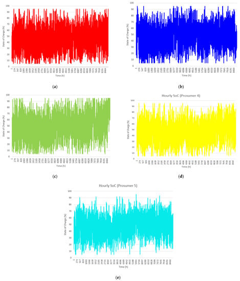
Figure 8.
Annual evolution of individual SoCs. (a) SoC of User 1; (b) SoC of User 2; (c) SoC of User 3; (d) SoC of User 4; (e) SoC of User 5.
Regarding daily SoC control, Figure 9 shows how the SoC would evolve according to the hourly differences between production and consumption and the current SoC value.
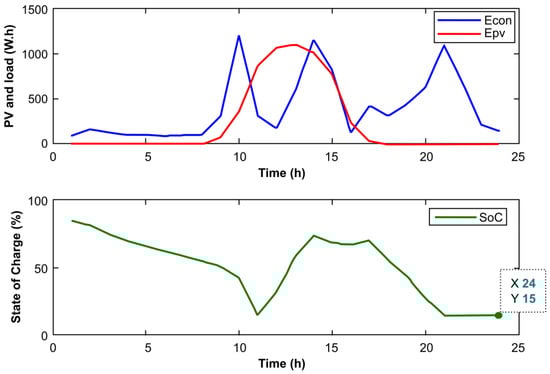
Figure 9.
Daily evolution of individual SoCs according to PV and consumption binomial.
According to the results, it has been demonstrated that the SoC is calculated correctly for each time-step and becomes limited if no energy is available inside. It should be noted that Figure 9 represents the day-ahead scheduling of one prosumer because discharging was stopped when the lower limit of 15% was reached.
3.4.2. Discussion
The economic results from case-study analysis are the indicators that:
- demonstrate which of the future energy consumption modalities or scenarios should be the most cost-effective from the consumer point of view;
- provide the opportunity to understand the relevance of the sizing of RES facilities, i.e., to see what kind of prosumers would be susceptible to adopting this kind of modality;
- identify the main drivers that would enable profitability of the proposed strategy and the rest of the scenarios.
Table 8 represents the associated expenses for each of the study cases/prosumers and the comparison between them.
Table 8.
Economic results of the 15-year study-case analysis.
As presented in Table 8 prosumers with very low annual energy consumption (<2000 kWh) values would increase their COE or expenses for energy supply. The rest of the users, who have higher consumption levels, would reduce their energy expenses and therefore would benefit from the proposed community model.
Another remarkable result is the wide difference between C and D study cases. It was determined that the higher the energy consumption level is, the greater such differences become. Therefore, knowing that the same investment costs have been faced, it can be concluded that the overrun is simply due to ineffective energy trading. Thus, investment-cost reduction, CIM-expense diminishment and different aFRR-market-intervention strategies must be considered key factors in achieving profitability.
Figure 10 shows the percentage breakdown of energy costs obtained in study case D for the three main consumption profiles (low, medium and high) that can be differentiated in the proposed community:
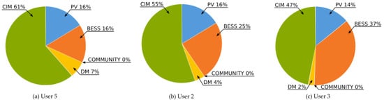
Figure 10.
Case study D total energy cost percentage breakdown of the main three consumption profiles analysed (high, medium and low).
As can be deducted, the weight of investment costs over the total increases the lower the energy needs are. Conversely, high consumption profiles require a much higher expense for energy market trading, mainly in CIMs. This fact along with economy-scale advantage they have, make investment costs less relevant compared to the other types of consumers. Nevertheless, excessive energy trading distances them from profitability in a higher grade in comparison with low to mid-consumers. As to tendencies between study scenarios, the same patterns were identified between scenarios B and C. The weight of the investment decreases and the trade increases accordingly as facility size grows.
Regarding sensible parameters, it is hard to find a combination of drivers that build a realistic scenario where the proposed EMS results are cost-effective for all kind of consumers. Nevertheless, it could be reachable for some of them. For instance, a scenario where PV and BESS total costs decrease reasonably could benefit the whole community.
It can be concluded that nowadays simplified compensation mechanisms are regarded as the most cost-effective solution for consumption levels above 2000 kWh/yr. The obtained results are profitable for mid- to high-consumption levels and slight modifications in market intervention and/or tariff structure could help further improve that goal. Low consumption levels do not seem to be susceptible to be part of the proposed community-based model.
4. Conclusions
Regarding home and community management, it has been demonstrated that the proposed strategy is profitable, technically viable and easily scalable for different community configurations and scenarios.
Despite not having reached cost-effectiveness for all the proposed cases, it has been demonstrated that the strategy is perfectly suitable from the technical point of view and compatible with existing schemes. Furthermore, market timing has been respected and, therefore, the EMS is in concordance with the energy markets it has been participating in.
As has been demonstrated, although not all consumers are suitable for the adoption of the proposed model due to the excessive weight of investment costs, having such wide differences in storage capacities is a huge drawback for the aggregator in terms of operability. In addition, these differences can provoke inequalities between community members that could arise from uneven cooperation situations; i.e., some users would support the community to a higher degree because of having a bigger storage capacity.
The proposed exchange methods are perfectly applicable in a collective self-consumption scheme where dynamic coefficients for prosumers are finally deployed. This condition is necessary in order to harness all the potential of self-consumption in most kinds of modalities because, by their adoption, much higher self-sufficiency and RES penetration would be achieved.
Author Contributions
Conceptualization, I.A.; Methodology, I.A., J.G.-C. and J.M.; Software, A.Z.; Validation, A.Z. and J.M.; Formal analysis, J.M.; Investigation, I.A.; Resources, I.L.; Writing—original draft, I.A.; Writing—review & editing, J.M., A.F.-A. and H.G. All authors have read and agreed to the published version of the manuscript.
Funding
This work is financially supported by the Basque Government under the Grant IT1647-22 (ELEKTRIKER research group), and by the Ministerio de Ciencia e Innovación, the Agencia Estatal de Investigación and the European Union under the Grant TED2021-129930A-I00 funded by MCIN/AEI/ 10.13039/501100011033 and by the “European Union NextGenerationEU/PRTR”.
Data Availability Statement
Not applicable.
Conflicts of Interest
The authors declare no conflict of interest.
References
- IRENA. Renewable Power Generation Costs in 2018; International Renewable Energy Agency: Abu Dhabi, United Arab Emirates, 2019. [Google Scholar]
- IRENA. Innovation Landscape for a Renewable-Powered Future: Solutions to Integrate Variable Renewables; International Renewable Energy Agency: Abu Dhabi, United Arab Emirates, 2019. [Google Scholar]
- Yavuz, L.; Önen, A.; Muyeen, S.M.; Kamwa, I. Transformation of Microgrid to Virtual Power Plant—A comprehensive review. IET Gener. Transm. Distrib. 2019, 13, 1994–2005. [Google Scholar] [CrossRef]
- Ramli, M.A.M.; Bouchekara, H.R.E.H.; Alghamdi, A.S. Optimal sizing of PV/wind/diésel hybrid microgrid system using multi-objective self-adaptative differential evolution algorithm. Renew. Energy 2018, 121, 400–411. [Google Scholar] [CrossRef]
- Logenthiran, T.; Srinivasan, D.; Khambadkone, A.M.; Aung, H.N. Multiagent System for Real-Time Operation of a Microgrid in Real-Time Digital Simulator. IEEE Trans. Smart Grid 2012, 3, 925–933. [Google Scholar] [CrossRef]
- Hatziargyriou, N.D.; Dimeas, A.; Tsikalakis, A.G.; Lopes, J.A.P.; Kariniotakis, G.; Oyarzabal, J. Management of Microgrids in Market Environment. In Proceedings of the 2005 International Conference on Future Power Systems, Amsterdam, The Netherlands, 16–18 November 2005. [Google Scholar]
- Zhou, Y.; Wei, Z.; Sun, G.; Cheung, K.W.; Zang, H. A robust optimization approach for integrated community energy system in energy and ancillary service markets. Energy 2018, 148, 1–15. [Google Scholar] [CrossRef]
- Maleki, A.; Khajeh, M.G.; Ameri, M. Optimal sizing of grid independent hybrid renewable energy system incorporating resource uncertainty and load uncertainty. Electr. Power Energy Syst. 2016, 83, 514–524. [Google Scholar] [CrossRef]
- Hosseinalizadeh, R.; Shakouri, H.; Amalnick, M.S.; Taghipour, P. Economic sizing of a hybrid (PV-WT-FC) renewable energy system (HRES) for stand-alone usages by an optimization-simulation model: Case study of Iran. Renew. Sustain. Energy Rev. 2016, 54, 139–150. [Google Scholar] [CrossRef]
- Maleki, A.; Askarzadeh, A. Artificial bee swarm optimization for optimum sizing of stand-alone PV/WT/FC hybrid system considering LPSP concept. Solar Energy 2014, 107, 227–235. [Google Scholar] [CrossRef]
- Di Somma, M.; Graditi, G.; Heydarian-Forushani, E.; Shafie-khah, M.; Siano, P. Stochastic optimal scheduling of distributed energy resources with renewables and considering economic and environmental aspects. Renew. Energy 2018, 116, 272–287. [Google Scholar] [CrossRef]
- Rezvani, A.; Gandomkar, M.; Izadbakhsh, M.; Ahmadi, A. Environmental/economic scheduling of a micro-grid with renewable energy resources. J. Clean. Prod. 2015, 87, 216–226. [Google Scholar] [CrossRef]
- Katsigiannis, Y.A.; Georgilakis, P.S.; Karapidakis, E.S. Multiobjetive genetic algorithm solution to the optimum economic and environmental performance problem of small autonomous hybrid power systems with renewables. IET Renew. Power Gener. 2010, 4, 404–419. [Google Scholar] [CrossRef]
- Phurailatpam, C.; Rajpurohit, B.S.; Wang, L. Planning and optimization of autonomous DC microgrids for rural and urban applications in India. Renew. Sustain. Energy Rev. 2018, 82, 194–204. [Google Scholar] [CrossRef]
- Aluisio, B.; Dicorato, M.; Forte, G.; Trovato, M. An optimization procedure for Microdrid day-ahead operation in the presence of CHP facilities. Sustain. Energy Grids Netw. 2017, 11, 34–45. [Google Scholar] [CrossRef]
- Gul, E.; Baldinelli, G.; Bartocci, P.; Bianchi, F.; Piergiovanni, D.; Cotana, F.; Wang, J. A techno-economic analysis of a solar PV and DC battery storage system for a community energy sharing. Energy 2022, 244, 123191. [Google Scholar] [CrossRef]
- Sarmiento, J.; Torres, E.; Larruskain, D.; Molina, M.P. Applications, Operational Architectures and Development of Virtual Power Plants as a Strategy to Facilitate the Integration of Distributed Energy Resources. Energies 2022, 15, 775. [Google Scholar] [CrossRef]
- Chaudhry, S.; Surmann, A.; Kühnbach, M.; Pierie, F. Renewable Energy Communities as Modes of Collective Prosumership: A Multi-Disciplinary Assessment, Part I—Methodology. Energies 2022, 15, 8902. [Google Scholar] [CrossRef]
- Chaudhry, S.; Surmann, A.; Kühnbach, M.; Pierie, F. Renewable Energy Communities as Modes of Collective Prosumership: A Multi-Disciplinary Assessment Part II—Case Study. Energies 2022, 15, 8936. [Google Scholar] [CrossRef]
- Fonseca, T.; Ferreira, L.L.; Landeck, J.; Klein, L.; Sousa, P.; Ahmed, F. Flexible Loads Scheduling Algorithms for Renewable Energy Communities. Energies 2022, 15, 8875. [Google Scholar] [CrossRef]
- Hosseini, S.M.; Carli, R.; Jantzen, J.; Dotoli, M. Multi-block ADMM Approach for Decentralized Demand Response of Energy Communities with Flexible Loads and Shared Energy Storage System. In Proceedings of the 2022 30th Mediterranean Conference on Control and Automation (MED), Athens, Greece, 28 June–1 July 2022; pp. 67–72. [Google Scholar]
- Hosseini, S.M.; Carli, R.; Dotoli, M. Robust Optimal Energy Management of a Residential Microgrid Under Uncertainties on Demand and Renewable Power Generation. IEEE Trans. Autom. Sci. Eng. 2021, 18, 618–637. [Google Scholar] [CrossRef]
- Euskalmet-Agencia Vasca de Meteorología, “Datos de estaciones”. Available online: https://www.euskalmet.euskadi.eus/inicio/ (accessed on 1 September 2022).
- i·DE Grupo Iberdrola. Available online: https://www.i-de.es/ (accessed on 1 September 2022).
- e·sios-Sistema de Información del Operador del Sistema. Available online: https://www.ree.es/es/actividades/operacion-del-sistema-electrico/e-sios (accessed on 1 September 2022).


Disclaimer/Publisher’s Note: The statements, opinions and data contained in all publications are solely those of the individual author(s) and contributor(s) and not of MDPI and/or the editor(s). MDPI and/or the editor(s) disclaim responsibility for any injury to people or property resulting from any ideas, methods, instructions or products referred to in the content. |
© 2023 by the authors. Licensee MDPI, Basel, Switzerland. This article is an open access article distributed under the terms and conditions of the Creative Commons Attribution (CC BY) license (https://creativecommons.org/licenses/by/4.0/).