Abstract
The interior permanent magnet synchronous machine (IPMSM) has been widely used in industrial applications due to its several favorable advantages. To further improve the machine performance, an improved nonlinear predictive controller for the IPMSM is proposed. In this paper, the maximum torque per ampere control law is firstly transformed to a linear function, according to the first−order Taylor expansion, and integrated with the control strategy. On this basis, an improved predictive control method is formulated by designing an optimized cost function through the input−output feedback linearization. Then the integral action is introduced to eliminate the influence of the load mutation and improve the steady−state control precision of the system. The stability of the control method is ensured by compelling the outputs to track the desired references without steady−state error. Finally, the simulation was established to verify the effective of the improved control method. Simulation results showed that the machine can reach the given reference speed without steady−state error within a short process, which means the machine has excellent dynamic and static performances. Furthermore, the machine has higher torque−to−current ratio by making full use of the reluctance torque. The simulation results verify the effectiveness of the improved control strategy.
1. Introduction
Currently, the permanent magnet synchronous machine (PMSM) is widely used in industrial applications due to its favorable advantages, such as high power density, high efficiency and good controllable performance [1,2,3]. On some occasions, the PMSM is forced to track the desired speed, whose performance is influenced by the control policy. To increase the machine performance, many control methods have been proposed, including proportional control [4,5], sliding mode control (SMC) [6,7] and predictive control [8,9].
PI control is a classic control strategy providing such advantages as good robustness and high steady−state control precision, whereas its dynamic performance is influenced by the controller parameters. The PMSM is a complex nonlinear system operating in a wide speed range with inevitable disturbances and parameter uncertainties. Hence, a PI control with fixed regulation parameters cannot achieve a satisfying dynamic performance during the entire running process. The SMC has been widely used in some practical applications because of its high response speed and powerful ability to eliminate some disturbances. In [7], a compound control method using improved non−singular fast terminal SMC and disturbance observer compensation techniques was developed. In [10], the nonlinear control strategy for PMSM was proposed by adopting a fast terminal SMC based on the finite time sliding mode observer. In [11], an improved SMC was proposed to promote the drive performance of PMSM. Comprehensive simulation verified that the proposed controller was strongly robust to acute variations of load and machine parameters. In [12], a terminal SMC based on nonlinear disturbance observer is proposed to realize the speed and the current tracking control for the PMSM drive system. However, it is difficult for the SMC to overcome the influence of certain parameter uncertainties not satisfying the matching condition.
The model predictive control (MPC) is an optimization−based control strategy with strong robustness. It can predict future output through the input−output feedback linearization. On this basis, a cost function to evaluate the difference between the predicted output and the trajectory to be tracked is designed, whose optimal solution serves as the input of the system. The PMSM is a nonlinear multivariable system with fast dynamic, and it is sensitive to the disturbances and parameter mismatches. Hence, the discrete time linear MPC in [13] suffers from several limitations, such as the unavoidable steady−state error and high computational effort.
In order to improve the control performance, some improved MPC methods have been put forward [14,15,16]. In [17], a cascade MPC structure including the inner current loop and outer speed loop was developed. Typically, the speed loop MPC is embedded with different disturbance frequency modes to reduce the effect of periodic disturbance. In [18], the model of predictive direct current control based on an optimized cost function is proposed, which can achieve fast dynamic in transient state and reduce the converter losses in steady state. In [19], a cascade−free modulated predictive direct speed control scheme for PMSM drives is presented to improve the machine steady−state performance. In [20], a novel MPC mechanism referred as the Runge–Kutta MPC has been applied for speed control of a commercial PMSM. In [21], an improved MPC method is incorporated into the control design of the speed loop of PMSM, in which a compensated scheme with an extended sliding mode observer is added. In [22], a current MPC is designed for a PMSM where the speed of the motor can be regulated precisely.
The disturbance observer has been proven to be effective in estimating the bounded disturbance [23], and some papers have combined the MPC with the disturbance observer to suppress the effects of external perturbation. In [24], a composite control method combining the deadbeat predictive control and stator current observer is designed, which can reduce the control error caused by model parameter mistake and one−step delay. Another effective way to improve the disturbance attenuation is to bring in the integral action to the MPC [25]. In [26], a robust nonlinear predictive control method is proposed, which introduces the integral item by designing an optimized cost function. The simulation results verify the high performance of the controller in the presence of disturbance and mismatched parameters.
It should be noticed that the mentioned control strategies apply to the surface−mounted PMSM (SPMSM). The d-axis and q-axis inductance of SPMSM are equal, and hence, these controllers can achieve the maximum torque per ampere ratio by impelling the d-axis current to zero. As for the IPMSM, the d-axis and q-axis inductance are not equal. Hence, these predictive controllers cannot make full use of the reluctance torque caused by the interaction of the unequal d-axis and q-axis inductance. In addition, it is necessary to improve the predictive controllers to improve the torque−to−current ratio.
To improve the torque−to−current ratio of IPMSM, a nonlinear predictive control strategy with an improved cost function is proposed in this paper. By integrating the maximum torque per ampere (MTPA) control law with the predictive control strategy, the controller can make full use of the reluctance torque of IPMSM. The controller is verified to have excellent static and dynamic performance. The main content is organized as follows: In Section 2, the mathematical model of the IPMSM is presented. On this basis, the MTPA control law is expounded and transformed to a linear constraint for the armature current. Combined with the mentioned current constraint, an optimized predictive controller applied to the IPMSM is proposed in Section 3. In order to eliminate the steady−state error caused by the load mutation, the integral term is also brought in by designing a revised cost function. Section 4 gives the simulation results of the controller. In addition, the corresponding conclusion is drawn in Section 5.
2. Linear Constraint of the Armature Current
The mathematical model of the IPMSM can be depicted in dq coordinate system by
where ud, uq are the d-axis and q-axis components of the armature voltage; id, iq are the d-axis and q-axis components of the armature current; R, Ld and Lq are the phase resistance, the d-axis and q-axis inductances, respectively; p is the number of pole pairs; ω is the rotor angular speed; ψf represents the permanent magnet flux; J, B and TL are the moment of inertia, the coefficient of friction and the load torque, respectively. The specific parameters of the machine studied in this paper are listed in Table 1.

Table 1.
Main parameters of the machine.
For the IPMSM, there exists the reluctance torque component if id is not zero. So, it is not the best choice to adopt the common current controller which forces the d-axis current to zero. To get the maximum output torque under the minimum current, the maximum torque per ampere (MTPA) control is adopted in this paper.
The equations of the MTPA can be expressed as
where is and Te are the armature current and the electromagnetic torque, respectively. The Lagrange multiplier is adopted to solve this equation, which is expressed as
where λ is the Lagrange multiplier. Then, the partial derivatives of H(id, iq, λ) with respect to id, iq and λ are
Set the partial derivative equations equal to zero; it yields that
Equation (8) is a complex quartic equation about iq, whose solution can be obtained by the numerical method. It should be noticed that the value of iq is positive, whereas id is negative for the condition that Ld < Lq. The nonlinear curves of id and iq varying with Te are given in Figure 1.
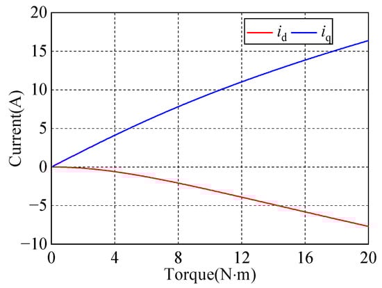
Figure 1.
Curves of id and iq varying with the electromagnetic torque.
In the steady state, the derivative of ω with respect to time is zero. So, the Equation (3) can be transformed into
The electromagnetic torque is approximately equal to the load torque. Under this condition, it can obtain the relational between the steady−state armature current and the load torque through polynomial curve fitting method.
where ids_r, iqs_r are the estimated values of ids, iqs, respectively. The values of the coefficients in Equation (10) are d1 = 7.463 × 10⁻⁴, d2 = −0.031, d3 = −0.071, d4 = 0.084, and q1 = −0.013, q2 = 1.076, q3 = 0.012. Figure 2 exhibits the comparison between the numerical and curve fitting solutions of ids and iqs, respectively. The results achieved by the two methods agree well with each other, which verifies the high precision of the curve fitting method.
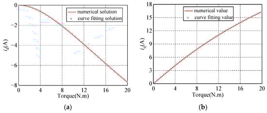
Figure 2.
The numerical and curve fitting solutions of (a) id; (b) iq.
The PM machine mainly operates in steady state with the required speed. So, it is reasonable to give priority to the correlation between the d-axis and q-axis steady−state current. It can assume that the d-axis and q-axis armature current are ids and iqs, respectively, when the machine runs steadily with a given load torque. Then, Equation (10) can be transformed into a piecewise function based on the first−order Taylor expansion, which is diagrammed in Figure 3. For a certain interval, the governing function about id and iq can be expressed as
where μ and ς are two coefficients determined by the load torque.
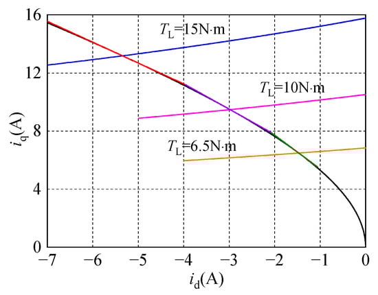
Figure 3.
The first-order Taylor expansion at the certain point.
3. Proposed Controller for the IPMSM
3.1. Design of the Controller
It can adopt Equation (11) as a linear constraint to the d-axis and q-axis armature current of the PM machine. Refer to [26]; the mathematical model of the IPMSM can be expressed as Equation (13). Herein, the constraint of (11) instead of id = 0 is adopted to determine the output parameters.
where x = [id iq ω]T are the state variables, u = [ud uq]T are the inputs, y = [h1(x) h2(x)]T are the outputs, and b denotes the disturbance caused by the load torque. The reference value of h1(x) is 0, and the reference value of h2(x) is the reference speed.
According to Equation (13), the following equations are derived based on the standard Lie derivative.
It is observed that Lg1h1(x) and Lg1Lfh2(x) are the non−singular matrixes. In addition, the elements of Lg1h2(x) are equal to zero. Hence, the relative degrees of the outputs y1 and y2 are ρ1 = 1 and ρ2 = 2, respectively. The total relative degree of the nonlinear system is ρ = ρ1 + ρ2 = 3, which is equal to the number of state variables. Therefore, the nonlinear system can be transformed into a linear model through the input−output feedback linearization. Based on the standard Lie derivative, the ρi−time derivatives of the outputs yi with respect to time are given by
The outputs of the machine are forced by the controller to track the reference trajectory in the predictive period. For this purpose, a cost function should be firstly designed, whose optimum solutions serve as the inputs to the system. As stated in [25], the integral action can eliminate the steady error caused by the disturbance and parameter uncertainty. Herein, the integral term is introduced to the controller by defining a generalized cost function.
where T1 and T2 are the prediction horizons for the current loop and speed loop, respectively. The response speed of the current loop is much faster than the speed loop, so T1 can be set to a positive number smaller than T2.
where c1, c2, c3 and c4 are the coefficients to be designed, and yi_r is the desired reference.
Substituting Equation (19) into Equation (20), the cost function given in Equation (20) transforms to
where
Taking partial derivative of M with respect to u gives
The solutions of the equation ∂M/∂u = 0 are the optimal values such that the cost function is minimized. By solving the function ∂M/∂u = 0, the input voltage of the machine can be determined by
3.2. Constraints of the Controller
The capacity of the inverter is limited. During the transient process, the armature voltage and current may exceed its limit values. Hence, the necessary constraints should be added to the control system. The upper and lower bound limits are chosen based on the maximum output voltage and maximum output current of the inverter. By this method, the machine voltage and current are within the required range, which avoids the damage of excess current to the inverter.
As the armature current id and iq are the state variables and cannot be constrained directly, the current constraints can be achieved by setting proper limitations to the input voltage. The Lie derivatives of the armature current along the field vector g1 are given by
Equation (34) implies that the relative degrees of the armature current id and iq to the input variables are ρ3 = 1 and ρ4 = 1, respectively. So, the predicted current can be expanded into the first−order Taylor series as
The predicted current id(t + τ) and iq(t + τ) satisfy the inequality constraints given in Equation (33). Substituting Equation (33) into Equation (35) yields
Equation (32) together with Equations (36) and (37) constitute the constraints to the proposed controller.
3.3. Stability Analysis
Assume that the disturbance b(t) is bounded. As for the nonlinear system for Equation (13), it can be concluded that the closed loop system under the proposed control law is asymptotically stable. In addition, the outputs will track the desired references with the error approaching zero asymptotically. The proof process is summarized briefly in the following.
The first order derivative of h1(x) along the vector g2 is given by
Combing Equation (31) with Equation (39), the following function about the error e1 is derived.
where
The real parts of the eigenvalues of A1 are negative, indicating that the current loop under the control law (31) is Hurwitz asymptotically stable. On this basis, the error e1 will converge to zero if t→∞ deduced from the Barbalat lemma [27].
Taking the disturbance into consideration, the first and second order Lie derivatives of y2 are given by
Substituting Equation (31) into Equation (43), we can get the governing equation of the error e2 as
where
A2 is a Hurwitz matrix, so there exists a symmetric positive matrixes P, such that
Then, establish a Lyapunov function candidate as
The derivative of V2 with respect to time is expressed as
where ξ = ‖P‖ is a positive value.
Under the condition that b(t) and B(x) are bounded, it can be deduced that the derivative of V2 with respect to time is negative if the integral of e2 is sufficiently large, which shows that the speed loop is asymptotically stable despite the existence of disturbance. Similarly, the output error e2 satisfies e2(t) = 0 when t→∞.
4. Simulation Analysis
The block diagram of the IPMSM predictive control system is shown in Figure 4. To verify the effectiveness of the proposed control method (strategy 1), a comparison with the robust nonlinear predictive controller [26] (strategy 2) is carried out.
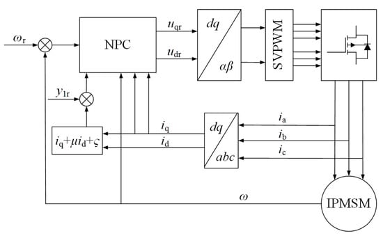
Figure 4.
The block diagram of the predictive control system.
The prediction horizon of the current loop T1 is set to 1ms, whereas that of the speed loop T2 is 5 ms. The sampling time of the system is 0.01ms. It should be noticed that the integral gain c1 and c2 would influence the machine performance. The bigger integral gain will improve the response speed but may cause the undesired overshoot. However, an unfavorable decrease in the integral gain would enlarge the setting time of the system.
During the simulation process, the load torque is set to 5 N·m and the speed reference is 100 rad/s. Figure 5 exhibits the speed response of the IPMSM with two control methods. It can be observed from Figure 5a that the machine can reach the reference speed within a very short period, indicating that the system has excellent dynamic and static performances with strategy 1. Control strategy 2 has similar response speed during the start−up process. However, the phase current would exceed its limited value for this condition. Figure 6 shows the d-axis and q-axis components of the armature current with control strategy 1 and strategy 2. It can be seen that the d-axis current under strategy 2 maintains to zero. By comparison, the d-axis current is not zero but a negative value when strategy 1 is employed.
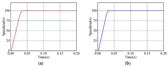
Figure 5.
The speed response of the machine with (a) control strategy 1; (b) control strategy 2.
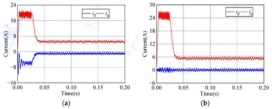
Figure 6.
The d-axis and q-axis current with (a) control strategy 1; (b) control strategy 2.
The three phase currents with control strategy 1 and strategy 2 are compared in Figure 7. As stated in [26], strategy 2 is an unconstrained controller, and the speed response of this control strategy is related to the gradient of the speed trajectory. When the speed trajectory is changing quickly, the armature current would exceed its limit value during the dynamic process, which is reflected clearly in Figure 7b. So, the speed trajectory must be chosen to keep the armature current within its threshold, and the integral gain needs to be adjusted simultaneously. However, the change of integral gain would affect the machine performance. In addition, it is difficult to obtain the appropriate value of these parameters. By comparison, the strategy 1 proposed in this paper solves this problem by adding the voltage and current constraints.
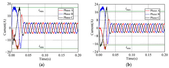
Figure 7.
The phase current with (a) control strategy 1; (b) control strategy 2.
In addition, Figure 8 gives the speed response and armature current curves when the gradient of the speed trajectory is slow with strategy 2. As shown in Figure 8b, the armature current is limited within the threshold value. However, it takes more time for the machine to reach the steady state, which has an adverse influence on the machine dynamic performance. By contrast, the machine with strategy 1 could approach the steady state within 0.05 s, indicating that a better dynamic performance is achieved with the proposed control method.
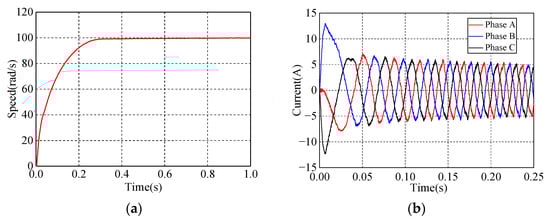
Figure 8.
The (a) speed response; and (b) phase current with control strategy 2 of slow speed trajectory.
For further verification, the load torque of the machine is set to 5 N·m originally, but stepped up to 20 N·m at 1 s. Figure 9 gives the speed response and the phase current curves of the machine, respectively. It can be seen that it takes about 1 s for the steady−state error to maintain to zero as the load torque is increased suddenly up to 400%. Figure 10 shows the d-axis and q-axis components of the current corresponding to the proposed controller. In the steady state, as clearly shown in Figure 10, the d-axis current maintains to about −8A, whereas the q-axis current turns into 16A, approximately. In addition, the two components of the armature current id and iq satisfy the linear constraint given in Equation (9). Figure 11 compares the A phase armature current when the machine operates with the reference speed. The machine is controlled by two different control strategies. On the premise of obtaining the same electromagnetic torque, it is obvious that the steady−state armature current under strategy 1 is smaller than that of strategy 2. It indicates that the proposed controller has a higher torque−to−current ratio than the other control strategy.
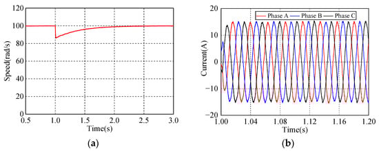
Figure 9.
The (a) speed response; and (b) phase current with control strategy 1 under load mutation.
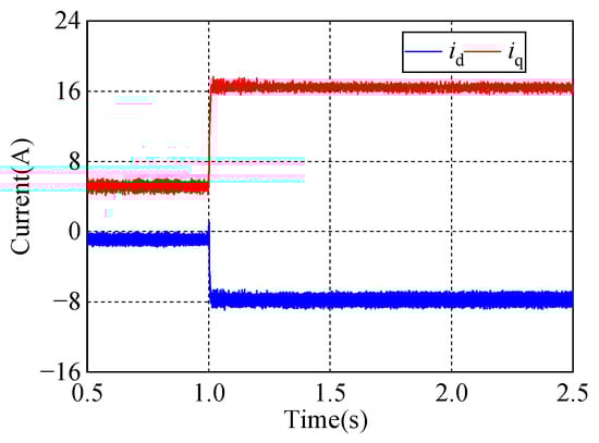
Figure 10.
The d-axis and q-axis current with control strategy 1.
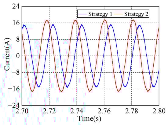
Figure 11.
The A phase current with the two different controllers.
Then, the speed response of the machine for step speed change and rapid speed change conditions are researched. The reference speed is set to 100 rad/s originally, but stepped up to 110 rad/s and 200 rad/s at 1 s, respectively. Figure 12 gives the speed response of the machine. As shown in Figure 12a, the machine can reach the reference speed within 0.02 s without overshoot. For the rapid speed change condition, the machine speed would approach the reference speed rapidly with a little overshoot. Then, the static speed error is eliminated within 0.1 s. Simulation results indicate that the machine has excellent dynamic performances for speed change condition.
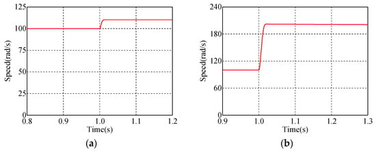
Figure 12.
The speed response for (a) step speed change condition; and (b) rapid speed change condition.
The load torque is set to rated load and the speed reference is rated speed. Figure 13a exhibits the speed response of the IPMSM with the proposed control strategy, and Figure 13b gives the phase current when the machine operates with rated speed and full load. As can be seen in Figure 13, the machine can operate with full load at rated speed. Furthermore, it can be observed from Figure 13a that the machine can reach the rated speed within 1.5 s. The response time is short. Moreover, the machine can reach the rated speed without overshoot, which indicates that the machine has excellent dynamic performances with the proposed control strategy.
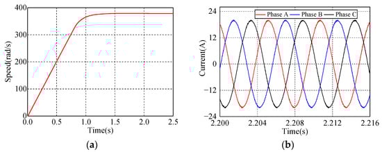
Figure 13.
The (a) speed response; and (b) phase current with proposed control strategy.
Simulation results indicate that: (1) the machine with the proposed controller can reach the specified speed rapidly during the start−up process, and the phase current is within its limited value; (2) the machine can eliminate the disturbance resulting from load change within a short period; (3) the machine can rapidly reach the reference speed for speed change conditions; (4) the machine has a higher torque−to−current ratio. Hence, the machine has excellent dynamic and static performances with the proposed control strategy, which verifies the effectiveness of the control strategy.
5. Conclusions
An improved nonlinear predictive control method for the IPMSM was presented in this paper. To make full use of the reluctance torque of the machine, the d-axis and q-axis components of the armature current were compelled to follow the linear constraint derived by the maximum torque per ampere control rule and first−order Taylor expansion during the running process. On this basis, the predictive controller was established by defining a generalized cost function whose solutions served as the inputs to the system, and the integral term was also introduced to avoid the effect of the external perturbations. The stability of the proposed control method was proved by the Lyapunov function and the Barbalat lemma. The simulation was established to verify the effectiveness of the proposed control method. Simulation results showed that the system has excellent dynamic and static performances. The d-axis and q-axis components of the armature current satisfied the given linear constraint, indicating that the proposed controller has a higher torque−to−current ratio than the one that forced the d-axis current to zero.
Author Contributions
Conceptualization, M.T.; Data curation, M.T. and H.C.; Formal analysis, M.T. and W.Z.; Investigation, M.T. and J.R.; Methodology, M.T.; Project administration, M.T.; Supervision, M.T.; Validation, M.T.; Visualization, W.Z.; Writing—original draft, M.T.; Writing—review and editing, H.C., W.Z. and J.R. All authors have read and agreed to the published version of the manuscript.
Funding
This research was funded by the Shandong Provincial Natural Science Foundation, China, grant number ZR2021QE057.
Data Availability Statement
Not applicable.
Conflicts of Interest
The authors declare no conflict of interest.
References
- Wu, L.; Yin, H.; Wang, D.; Fang, Y. A nonlinear subdomain and magnetic circuit hybrid model for open−circuit field prediction in surface−mounted PM machines. IEEE Trans. Energy Convers. 2019, 34, 1485–1495. [Google Scholar] [CrossRef]
- Hajdinjak, M.; Miljavec, D. Analytical calculation of the magnetic field distribution in slotless brushless machines with U−shaped interior permanent magnets. IEEE Trans. Ind. Electron. 2020, 67, 6721–6731. [Google Scholar] [CrossRef]
- Peng, B.; Wang, X.; Zhao, W.; Ren, J. Study on shaft voltage in fractional slot permanent magnet machine with different pole and slot number combinations. IEEE Trans. Magn. 2019, 55, 8102305. [Google Scholar] [CrossRef]
- Riaz, S.; Lin, H.; Anwar, M.B.; Ali, H. Design of PD−type second−order ILC law for PMSM servo position control. J. Phys. Conf. Ser. 2020, 1707, 012002. [Google Scholar] [CrossRef]
- Liu, G.; Chen, B.; Wang, K.; Song, X. Selective current harmonic suppression for high−speed PMSM based on high−precision harmonic detection method. IEEE Trans. Ind. Informat. 2019, 15, 3457–3468. [Google Scholar] [CrossRef]
- Junejo, A.K.; Xu, W.; Mu, C.; Ismail, M.M.; Liu, Y. Adaptive speed control of PMSM drive system based a new sliding−mode reaching law. IEEE Trans. Power Electron. 2020, 35, 12110–12121. [Google Scholar] [CrossRef]
- Xu, B.; Zhang, L.; Ji, W. Improved non−singular fast terminal sliding mode control with disturbance observer for PMSM drives. IEEE Trans. Transp. Electrif. 2021, 7, 2753–2762. [Google Scholar] [CrossRef]
- Nawaz, M.K.; Dou, M.; Riaz, S.; Sardar, M.U. Current control of permanent magnet synchronous motors using improved model predictive control. Math. Probl. Eng. 2022, 2022, 1736931. [Google Scholar]
- Chen, W.-H.; Ballance, D.J.; Gawthrop, P.J. Optimal control of nonlinear systems: A predictive control approach. Automatica 2003, 39, 633–641. [Google Scholar] [CrossRef]
- Xu, W.; Junejo, A.K.; Tang, Y.; Shahab, M.; Habib, H.U.R.; Liu, Y.; Huang, S. Composite speed control of PMSM drive system based on finite time sliding mode observer. IEEE Access 2021, 9, 151803–151813. [Google Scholar] [CrossRef]
- Jiang, Y.; Xu, W.; Mu, C.; Liu, Y. Improved deadbeat predictive current control combined sliding mode strategy for PMSM drive system. IEEE Trans. Veh. Technol. 2018, 67, 251–263. [Google Scholar] [CrossRef]
- Liu, X.; Yu, H.; Yu, J.; Zhao, L. Combined speed and current terminal sliding mode control with nonlinear disturbance observer for PMSM drive. IEEE Access 2018, 6, 29594–29601. [Google Scholar] [CrossRef]
- Bolognani, S.; Peretti, L.; Zigliotto, M. Design and implementation of model predictive control for electrical motor drives. IEEE Trans. Ind. Electron. 2009, 56, 1925–1936. [Google Scholar] [CrossRef]
- Sun, C.; Sun, D.; Chen, W.; Nian, H. Improved model predictive control with new cost function for hybrid-inverter open-winding PMSM system based on energy storage model. IEEE Trans. Power Electron. 2021, 36, 10705–10715. [Google Scholar] [CrossRef]
- Xue, C.; Zhou, D.; Li, Y. Finite-control-set model predictive control for three-level NPC inverter-fed PMSM Drives with LC filter. IEEE Trans. Ind. Electron. 2021, 68, 11980–11991. [Google Scholar] [CrossRef]
- Abu−Ali, M.; Berkel, F.; Manderla, M.; Reimann, S.; Kennel, R.; Abdelrahem, M. Deep learning-based long-horizon MPC: Robust, high performing, and computationally efficient control for PMSM drives. IEEE Trans. Power Electron. 2022, 37, 12486–12501. [Google Scholar]
- Wang, L.; Chai, S.; Rogers, E.; Freeman, C.T. Multivariable repetitive -predictive controllers using frequency decomposition. IEEE Trans. Control Syst. Technol. 2012, 20, 1597–1604. [Google Scholar] [CrossRef]
- Preindl, M.; Schaltz, E.; Thogersen, P. Switching frequency reduction using model predictive direct current control for high power voltage source inverters. IEEE Trans. Ind. Electron. 2011, 58, 2826–2835. [Google Scholar] [CrossRef]
- Zheng, C.; Yang, J.; Gong, Z.; Xiao, Z.; Dong, X. Cascade-free modulated predictive direct speed control of PMSM drives. Energies 2022, 15, 7200. [Google Scholar] [CrossRef]
- Akpunar, A.; Iplikci, S. Runge-Kutta model predictive speed control for permanent magnet synchronous motors. Energies 2020, 13, 1216. [Google Scholar] [CrossRef]
- Shao, M.; Deng, Y.; Li, H.; Liu, J.; Fei, Q. Sliding mode observer-based parameter identification and disturbance compensation for optimizing the mode predictive control of PMSM. Energies 2019, 12, 1857. [Google Scholar] [CrossRef]
- Tang, M.; Zhuang, S. On speed control of a permanent magnet synchronous motor with current predictive compensation. Energies 2019, 12, 65. [Google Scholar] [CrossRef]
- Yang, J.; Zheng, W.X.; Li, S.; Wu, B.; Cheng, M. Design of a prediction-accuracy-enhanced continuous-time MPC for disturbed systems via a disturbance observer. IEEE Trans. Ind. Electron. 2015, 62, 5807–5815. [Google Scholar] [CrossRef]
- Zhang, X.; Hou, B.; Mei, Y. Deadbeat predictive current control of permanent-magnet synchronous motors with stator current and disturbance observer. IEEE Trans. Power Electron. 2017, 32, 3818–3834. [Google Scholar] [CrossRef]
- Hedjar, R.; Toumi, R.; Boucher, P.; Dumur, D. Finite horizon nonlinear predictive control by the Taylor approximation: Application to robot tracking trajectory. Int. J. Appl. Math. Comput. Sci. 2005, 15, 527–540. [Google Scholar]
- Errouissi, R.; Ouhrouche, M.; Chen, W.-H.; Trzynadlowski, A.M. Robust nonlinear predictive controller for permanent-magnet synchronous motors with an optimized cost function. IEEE Trans. Ind. Electron. 2012, 59, 2849–2858. [Google Scholar] [CrossRef]
- Tao, G. A simple alternative to the Barbalat lemma. IEEE Trans. Autom. Contr. 1997, 42, 698. [Google Scholar] [CrossRef]


Disclaimer/Publisher’s Note: The statements, opinions and data contained in all publications are solely those of the individual author(s) and contributor(s) and not of MDPI and/or the editor(s). MDPI and/or the editor(s) disclaim responsibility for any injury to people or property resulting from any ideas, methods, instructions or products referred to in the content. |
© 2023 by the authors. Licensee MDPI, Basel, Switzerland. This article is an open access article distributed under the terms and conditions of the Creative Commons Attribution (CC BY) license (https://creativecommons.org/licenses/by/4.0/).