Machine Learning Prediction of Nanoparticle Transport with Two-Phase Flow in Porous Media

Abstract

Reservoir simulation is a time-consuming procedure that requires a deep understanding of complex fluid flow processes as well as the numerical solution of nonlinear partial differential equations. Machine learning algorithms have made significant progress in modeling flow problems in reservoir engineering. This study employs machine learning methods such as random forest, decision trees, gradient boosting regression, and artificial neural networks to forecast nanoparticle transport with the two-phase flow in porous media. Due to the shortage of data on nanoparticle transport in porous media, this work creates artificial datasets using a mathematical model. It predicts nanoparticle transport behavior using machine learning techniques, including gradient boosting regression, decision trees, random forests, and artificial neural networks. Utilizing the scikit-learn toolkit, strategies for data preprocessing, correlation, and feature importance are addressed. Furthermore, the GridSearchCV algorithm is used to optimize hyperparameter tuning. The mean absolute error, R-squared correlation, mean squared error, and root means square error are used to assess the models. The ANN model has the best performance in forecasting the transport of nanoparticles in porous media, according to the results.

1. Introduction

The global demand for energy, including oil and natural gas, has increased in recent decades. The world’s energy demand is constantly increasing, and technical development for finding new reservoirs or developing improved oil recovery techniques is always progressing [1]. Nanoparticles are employed in enhanced oil recovery since 60 to 70% of hydrocarbon in most oil fields is not recovered with primary and secondary recovery schemes [2]. For example, silica nanoparticles, which are ecologically safe, can improve oil recovery. Nanoparticles have some unique properties due to their tiny size, such as an increased surface area to which other materials can attach, resulting in stronger or lighter materials. However, some nanoparticles can be linked to rocks by surface filtration, straining, and physicochemical filtration, drastically lowering the porosity and permeability of the porous medium [2,3]. This is true even though the compact size of nanoparticles favors their transfer in porous media. Therefore, several factors, including nanofluid concentration, injection rate, slug size, and particle size, can affect the transportability of nanoparticles in pore throats. The flow of hydrocarbons in porous media has historically been estimated using numerical models; however, they have become challenging for more sophisticated numerical techniques. Recently, petroleum engineering has become one of the many industries where machine learning is frequently used. In order to create artificial datasets for machine learning algorithms to predict nanoparticle mobility, this study uses mathematical continuum models of nanoparticles in porous media. Artificial neural networks, gradient boosting regression, decision trees, random forests, and RF are the machine learning approaches utilized in the prediction throughout this study.

Nanotechnology provides a novel way to govern petroleum recovery processes. Nanoparticles can alter the fluid’s rheology, improving surfactant solution in EOR processes and lowering the interfacial tension between the aqueous phase and the oil interface [4,5]. By altering different rock and fluid characteristics, nanoparticles can improve hydrocarbon recovery. Nanoparticles can convert the rock’s wettability from oil-wet to water-wet [5]. Other features include conductivity alteration, rock and oil interaction, and wettability modification can also be modified. Moreover, changing the fluid’s viscosity, reducing the interfacial tension, and stabilizing the emulsion leads to an increase in recovery of more than 20% above conventional chemical surfactant-polymer flooding [6]. As the high temperature inside the reservoir decreases the effectiveness of surfactant and polymer flooding, the nanofluid combination exhibits a stable behavior at higher temperatures [7]. In oil-wet rocks, oil tends to adhere to the walls of porous media, making the waterflooding process useless since oil droplets cannot easily pass through the matrix’s pores. Recently, it was found that the introduction of nanoparticles can change the wettability of rock to water-wet. Water tends to imbibe to the rock surface in water-wet rock, and as a result of water flooding, oil flows toward the production well, improving oil recovery [8].

When nanoparticles are injected into the hydrocarbon reservoirs, it is important to understand their transport and properties to identify their mobility. The porous media utilized in laboratory research to study the transport of nanoparticles in porous media are columns filled with sand or glass beads. The retention of nanomaterials in those columns depends on the material size, shape, and surface characteristics. The dispersion of silica nanoparticles in polyacrylamide was discussed by Maghzi et al. [9]. The experiment examined the rheological characteristics of silica nanoparticles and polyacrylamide. They discovered an improvement in the polymers’ fluid viscosity and pseudoplastic behavior. The spreading behavior of nanofluids combined with surfactants on a solid surface was examined by Wasan and Nikolov [10]. Ju and Fan [11] observed the wettability alteration brought on by polysilicon nanoparticles using experimental and computational methods.

Youssif et al. [12] conducted experiments to investigate the effects of injecting silica nanoparticles with various concentrations and found that when the concentration of nanoparticles increases, the oil recovery factor increases. Khalilinezhad et al. [13,14] studied the impact of nanoparticles on the flow behavior of an injected flood in a porous medium using the UTCHEM simulator. They concluded that adding nanoparticles to polymers reduces sandstone retention and adsorption after using a polymer shear thinning model to assess the adsorption of nanoparticles on sandstone surfaces. Copper oxide nanoparticle transport in two-dimensional porous media was investigated by Jeong and Kim [15]. They looked at how pores gathered copper oxide nanoparticles. They found that nanoparticle flow velocity and surfactant concentration impacted how quickly they accumulated and deposited. Additionally, they discovered that the density affects the flow velocity such that the flow velocity decreases as the number of aggregates increases. Response surface techniques are employed to manage the Walters-B nanofluid stationary point flow brought on by a Riga surface [16]. Using capillary forces and Brownian diffusion, El-Amin et al. [17,18] developed a mathematical model for nanoparticle water suspensions in two-phase flow in porous media. As part of their investigation, they looked at how infused nanoparticles affected the properties of solids and fluids.

Machine Learning is a branch of artificial intelligence concerned with creating and developing algorithms that allow computers to learn behaviors or patterns from empirical data [19,20]. Traditionally, mathematical models are utilized to simulate hydrocarbon reservoirs. However, they are complicated and take a long time to compute [21]. Given the various computer platforms, parallel methods can help tackle such challenges. These issues could be solved using machine learning techniques. To forecast the nanofluid dynamic viscosity over different temperature ranges, Esfe et al. [22] built an artificial neural network model. A data-driven viscosity prediction model for water-based nanofluids was created by Changdar et al. [23] utilizing deep learning. Based on well-log data and stochastic gradient boosting regression, Subasi et al. [24] developed a machine-learning model to predict reservoir permeability. They explored various machine learning techniques, including random forest, artificial neural networks, K-nearest neighbors (KNN), support vector machine (SVM), and stochastic gradient boosting. They found that stochastic gradient boosting outperformed other assessed models in several evaluation metrics tests, including accuracy and root, mean squared error. Nanoparticle transport behavior in porous media was predicted by Zhou et al. [25] using a data-driven approach to construct the regression and classification models for nanoparticle retention and nanoparticle profiles. They employed one-hot encoding and random forest to fill in all the gaps in their dataset. They performed regression for predicting nanoparticle retention using the CatBoost technique in combination with synthetic minority oversampling. Goldberg et al. in [26] used the RF regression machine learning model to predict the nanoparticle concentration in a column length and the RF classification model to classify the nanoparticles retention profile shape of nanoparticles transport experiments in a fully saturated column, taking into consideration the physicochemical conditions such as nanoparticle size, coating type, and flow velocity. Irfan and Shafie [27] developed an ANN model to predict nanoparticle concentration. They built their dataset using the finite difference method simulator.

The current paper is structured as follows: Section 2 provides the research methodology. Section 3 presents the results and discussion. Finally, in Section 4, the conclusion is presented.

2. Research Methodology

The following actions were taken to perform this research: First, developing a mathematical model to simulate nanoparticle transport in porous media. Second, solving the model numerically and creating an artificial dataset for machine learning. Third, implementing selected machine learning techniques include gradient boosting regression, decision trees, random forests, and artificial neural networks to predict nanoparticle transport in porous media. Finally, performance evaluation metrics are used to assess the predictive models. The dataset is then subjected to preprocessing, eliminating whitespace, scaling, and noise. The dimensionality is decreased by choosing specific attributes. The training was then carried out utilizing the training dataset.

2.1. Machine Learning Modeling

A decision tree (DT) is a statistical machine learning approach used to solve classification and regression problems [28], implementing a sequential decision process. The tree’s branches, nodes, and leaves represent the DT model basics. The DT model mimics human thinking ability, making its tree-like structure easy to understand. The DT algorithm determines how many decision rules predict a result from a given set of inputs. The supervised ensemble machine learning technique known as random forest (RF) is frequently employed to address classification and regression problems. In RF, a large ensemble of decision trees collaborates to find a solution to a problem [29]. Therefore, the class with the most votes is chosen for perdition, and each decision tree produces a class prediction at random. RF computes the prediction average between trees in regression situations; it mixes numerous randomized decision trees and determines their predictions by averaging [30]. By averaging numerous unreliable and noisy trees, random forest improves estimating precision and reduces variation. Gradient boosting regression (GBR) is a learning model in which boosting might be represented as an optimization and explicit method [31]. Then, as an iterative functional gradient descent process, comprehensive functional gradient boosting strategies have been developed [32].

Artificial neural network (ANN) is a conceptual perspective that models the workings of the human brain by anticipating patterns and is inspired by biological neurons [33]. The ANN model is made up of fundamental processing nodes, or neurons, such that the learning method, network design, and transfer function are the three main parts of a neural network model [34]. Weighted connections between nodes can be changed as the network learns, and an activation function calculates each node’s output value based on its input values. Three common activation functions can be used in ANNs, including the hyperbolic tangent activation function, the sigmoid activation function, and the rectified linear unit activation function [35,36,37,38].

Table 1. Performance evaluation metrics.

Metric	Formula
Mean absolute error (MAE)	$\mathrm{MAE}=\frac{1}{n} {\displaystyle {\displaystyle \sum }_{i=1}^n}|actua{l}_i-predicte{d}_i|$
Mean squared error (MSE)	$\mathrm{MSE}=\frac{1}{n} {\displaystyle {\displaystyle \sum }_{i=1}^n}{(actua{l}_i-predicte{d}_i)}^2$
Root mean squared error (RMSE)	$\mathrm{RMSE}=\sqrt{\frac{1}{n} {\displaystyle {\displaystyle \sum }_{i=1}^n}{(actua{l}_i-predicte{d}_i)}^2}$
$\mathrm{R} \mathrm{squared} (R^2)$	$R^2=1-\frac{{\mathrm{MSE}}_{\mathrm{model}}}{{\mathrm{MSE}}_{\mathrm{base}}}$

presents some standard metrics to evaluate the performance of the used ML methods, including the R-squared (R²) correlation, mean absolute error (MAE), mean squared error (MSE), and root mean squared error (RMSE).

2.2. Traditional Mathematical Modeling

El-Amin et al. [18] developed a model to represent nanoparticle transport and a two-phase flow model in porous media. Darcy’s law is used to govern the two-phase flow in porous media. The mass conservation and continuity equations govern the two-phase flow in porous media. It is also called the saturation Equation (1) and Darcy’s equation or the momentum conservation Equation (2) [39],

$$\phi \frac{\partial S_{\alpha }}{\partial t}+\frac{\partial u_{\alpha }}{\partial z}=0$$

(1)

$$u_{\alpha }=-\frac{k_{r\alpha }}{{\mu }_{\alpha }} K(\frac{\partial P_{\alpha }}{\partial z}-{\rho }_{\alpha }g)$$

(2)

where $\alpha$ represents the phase oil or water, $\phi$ is the porosity of the medium, $p_{\alpha }$ is the density phase $\alpha$, $S_{\alpha }$ is the phase saturation, $u_{\alpha }$ is the phase velocity, $K$ is the absolute permeability, $k_{r\alpha }$ is the relative permeability of the phase, $P_{\alpha }$ is the phase pressure, $g$ is the gravitational acceleration, and ${\mu }_{\alpha }$ is the phase viscosity.

The relationship between oil saturation and water saturation is given as,

$$S_w+S_o=1$$

(3)

The difference between the pressures: $p_o$ (the non-wetting phase) and $p_w$ (the wetting phase) is the capillary pressure $p_c$,

$$p_c=p_o-p_w$$

(4)

El-Amin et al. in [39] considered taking the countercurrent imbibition where the overall velocity of water and oil is zero to simplify the saturation equation for the water phase Equation (1),

$$u_t=u_w+u_o=0$$

(5)

$$\varnothing \frac{\partial S_w}{\partial t}+\frac{\partial }{\partial z}\left[K {\lambda }_w{f}_o\left(\frac{\partial p_c}{\partial z}-\Delta \rho g\right)\right]=0$$

(6)

where ${\lambda }_w$ which is the mobility ratio of water, $f_o$ is the flow fraction of oil.

The normalized saturation is,

$$S=\frac{S_w-S_{iw}}{1-S_{or}-S_{iw}},\hspace{1em}0 < S < 1$$

(7)

where $S_{iw}$ is the irreducible water saturation, and $S_{or}$ is the reducible oil saturation.

The relative permeabilities are given by,

$$k_{rw}=k_{rw}^0{S}^a,k_{ro}=k_{ro}^0{(1-S)}^b$$

(8)

where $k_{rw}^0=k_{rw}\left(S=1\right)$ the relative permeability of water, and $k_{ro}^0=k_{ro}\left(S=0\right)$ the relative permeability of oil.

El-Amin et al. [39] wrote the nanoparticles transport in the water phase, assuming one size interval of nanoparticles as,

$$\phi \frac{\partial S_{w}C}{\partial t}+\frac{\partial }{\partial z}{u}_{w}C-\phi S_{w}D\frac{\partial C}{\partial z}=R$$

(9)

$$R=\frac{\partial C_{s1}}{\partial t}+\frac{\partial C_{s2}}{\partial t}$$

(10)

where $C$ is the volume concentration of nanoparticles in the water phase, $C_{s1}$ is the volume of nanoparticles in water available on pore surfaces per unit bulk volume of the porous medium, $C_{s2}$ is the volume of nanoparticles stuck in pore throats from the water phase per unit bulk volume of porous media due to bridging. Nanoparticles have strong Brownian motion because of their small size. Therefore, the diffusion dispersion tensor D is considered molecular diffusion $D_{diff}$ and hydrodynamic dispersion $D_{disp}$,

$$D=D_{diff}+D_{disp}$$

(11)

A surface deposition equation by Ju and Fan that took into consideration the critical velocity where only particle retention occurs, which is a modified version taken from Gruesbeck and Collins’s model [40], is given as,

$$\frac{\partial C_{s1}}{\partial t}=\{\begin{array}{c}{\gamma }_d\left|u_w\right|C,\hspace{1em}\hspace{1em}\hspace{1em}\hspace{1em}\hspace{1em}\hspace{1em}\hspace{1em}\hspace{1em}\hspace{1em}\hspace{1em}\hspace{1em}\hspace{1em}{u}_w\le u_c\hfill \\ {\gamma }_d\left|u_w\right|C-{\gamma }_e\left|u_w-u_c\right|C_{s1}, u_w>u_c\end{array}$$

(12)

where ${\gamma }_d$ is the nanoparticles surface retention in water coefficient, ${\gamma }_e$ is the entrainment coefficient of nanoparticles, $u_c$ is the critical velocity for the water phase, and the entrapment rate of nanoparticles in the water phase is,

$$\frac{\partial C_{s2}}{\partial t}={\gamma }_{pt}\left|u_w\right|C$$

(13)

where ${\gamma }_{pt}$ is the blocking constant of pore throat.

Porosity can be altered as a result of the deposition of nanoparticles on pore surfaces or pore throat blockage. The change in porosity can be written as,

$$\phi ={\phi }_0-\delta \phi , \delta \phi =C_{s1}+C_{s2}$$

(14)

where ${\phi }_0$ is the initial porosity.

As porosity changes, permeability also changes due to the deposition of nanoparticles on pore surfaces or blockage of pore throats [41].

$$K=K_0{\left[\left(1-f\right)k_f+f\frac{\phi }{{\phi }_0}\right]}^l$$

(15)

where $K_0$ is the initial permeability, $k_f$ is a constant for fluid seepage allowed by plugged pores.

The fraction of unplugged pores available for flow is the flow efficiency factor [18],

$$f=1-{\gamma }_f{C}_{s2}$$

(16)

where ${\gamma }_f$ is the nanoparticle’s flow efficiency coefficient. The exponent $l$ has a value in the range of 2.5 to 3.5.

Due to the nanoparticle retention in porous media, a variation in the relative permeability may occur. Ju and Fan in [11] calculated the specific area of a sand core and calculated the total surface area in contact with fluids for all nanoparticles size intervals per unit bulk volume,

$$a_{sp}=A\varphi {\left(\frac{\phi }{K}\right)}^{\frac{1}{2}}$$

(17)

$$a_{tot}=\frac{6 \beta }{d}\delta \phi$$

(18)

where A is the cross-sectional area, and d is the diameters of the nanoparticles in a given interval size. If $a_{tot}\ge$ $a_{sp}$, the total surfaces per unit bulk volume of porous media are fully covered with nanoparticles entrapped in pore throats or adsorbed on the pore surfaces. If $a_{tot}<$ $a_{sp}$, the surfaces per unit bulk volume of the porous medium are partially covered by the nanoparticles. Therefore, the water and oil relative permeability can be expressed as a linear function of the surface covered by the nanoparticles [18],

$$k_{rop}=k_{ro}+\frac{a_{tot}}{a_{sp}}\left(k_{ro,c }-k_{ro}\right)$$

(19)

$$k_{rwp}=k_{rw}+\frac{a_{tot}}{a_{sp}}\left(k_{rw,c }-k_{rw}\right)$$

(20)

where $k_{rop}$ is the oil relative permeability when the surface per unit bulk volume of porous media is completely occupied by nanoparticles, $k_{rwp}$ is the relative water permeability when the surface per unit bulk volume of porous media is completely occupied by nanoparticles [18],

$$k_{rw,c}={\theta }_w{k}_{rw}$$

(21)

$$k_{rop}=\left[1+\frac{a_{tot}}{a_{sp}}\left({\theta }_o-1\right)\right]k_{ro}$$

(22)

$$k_{rwp}=\left[1+\frac{a_{tot}}{a_{sp}} \left({\theta }_w-1\right)\right]k_{rw}$$

(23)

where ${\theta }_o$ is the ratio of the oil’s relative permeability due to nanoparticles adhering, and ${\theta }_w$ is the ratio of water relative permeability due to nanoparticles adhering.

The most popular correlations of capillary pressure are positive and restricted to primary drainage. Drainage refers to the decreasing saturation of a wetting phase, and imbibition refers to the increasing wetting-phase saturation. Skjaeveland et al. in [41] presented a general correlation for capillary pressure for mixed-wet reservoir rocks based on Brooks and Corey’s power-law form for primary drainage capillary pressure. The primary drainage starts from $S_w=1$, and the ptimary imbibition starts from $S_o=1$. El-Amin at al. [18] added both limiting expressions and wrote a general correlation:

$$p_c=\widetilde{b_w} {\left(\frac{S_w-S_{wr}}{1-S_{wr}}\right)}^{-a_w}+\widetilde{b_o} {\left(\frac{S_o-S_{or}}{1-S_{or}}\right)}^{-a_o}$$

(24)

where $\widetilde{b_w}$ (Pa) and $\widetilde{b_o}$ (Pa) are constants for the pressure entry of imbibition and drainage, respectively. The constants $\frac{1}{a_w}$ and $\frac{1}{a_o}$ are the imbibition and drainage pore size distribution index, respectively. The capillary pressure correlation can be written as in [18]:

$$p_c=b_w{\left(S+{ϵ}_1\right)}^{-a_w}+b_o{\left(1-S+{ϵ}_2\right)}^{-a_o}$$

(25)

where $b_w$ and $b_o$ are constants that depend on the constants $\widetilde{b_w}$ and $\widetilde{b_o}$. ${ϵ}_1$ and ${ϵ}_2$ are small numbers to correct the values of the capillary pressure at S = 0, and S = 1.

The water saturation at the beginning of the flow,

$$S_w=S_w^0 \mathrm{at} t=0, 0\le z\le H$$

(26)

where $S_W^0$ is the initial water saturation and $H$ is the rock depth.

The initial nanoparticle concentration is zero,

$$C=0 \mathrm{at} 0\le z\le H$$

(27)

The initial volume of nanoparticles available on pore surfaces and the initial volume of nanoparticles entrapped in pore throats due to bridging is given,

$$C_{s1}=C_{s2}=0 \mathrm{at} t=0, 0\le z\le H$$

(28)

$$s_W=1-S_o^0,c=c_0,C_{s1}=C_{s2}=0, \mathrm{at} t>0,z=0$$

(29)

$$\frac{d{S}_w}{dz}=\frac{dc}{dz}=\frac{d{C}_{s1}}{dz}=\frac{d{C}_{s2}}{dz}=0, \mathrm{at} t>0,z=h$$

(30)

where $C_0$ is the concentration of nanoparticles on the inlet boundary.

As a sample of running solving the numerical scheme, the water saturation and nanoparticles concentration are plotted against the pore volume in Figure 1. We can see that as nanoparticles’ concentration increases, the nanoparticles’ retention in porous media increases and reaches a steady flow. Moreover, the water saturation increases because nanoparticles are injected with water as a carrier to be transported in porous media.

3. Results and Discussion

The machine learning codes were written in Python3, implemented in Jupiter Notebook, and executed on a processor of 2.6 GHz Quad-Core Intel Core i7 and memory of 16 GB 2133 MHz LPDDR3. The execution time of DT and RF algorithms was super-fast, around a few seconds. The GBR execution time was 48.7 s. However, the ANN algorithm was more time-consuming, with an execution time of 18 min.

This section discusses the generation of the artificial datasets of the nanoparticle transport model. It covers how the dataset is preprocessed and scaled. It presents the use of features importance to identify the important features. This section also covers the use of different machine learning techniques, different target variables, and the performance evaluations of the models. After selecting the nanoparticles transport model in two-phase flow, the finite difference method is implemented to generate the artificial dataset. The generated dataset contains 288,000 instances for predicting different target variables, including nanoparticle concentration C, water saturation S_w, the relative permeability of oil K_rop, and the relative permeability of water K_rwp. Accordingly, we used the same datasets four times to predict the four different target variables: C, S_w, K_rop, and K_rwp. The two phase artificial dataset composed of 38 features or independent variables which are time (t), space (x), (phi₀) is the initial porosity, (phi) is the porosity of the medium, (rho_o) is the oil density, (rho_w) is the water density, (pc) is the capillary pressure, (k₀) is the initial permeability, (K) is the absolute permeability, (k_ro) is the oil relative permeability, (k_rw) is the water relative permeability, (k_ro0) is the initial oil relative permeability, (k_rw0) is the initial water relative permeability, (k_rwp) is the relative permeability of water when the surface of porous media is occupied nanoparticles, (k_rop) is the relative permeability of oil when the surface of the porous media is occupied with nanoparticles, (theta_w) is the ratio of the water relative permeability due to nanoparticles adhering, (theta_o) is the ratio of oil relative permeability due to nanoparticle adhering, (g) is the gravitational acceleration, (S_w) is the water saturation, (C) is the nanoparticles concentration in water, (C_s1) is the volume of nanoparticles in water, (C_s2) is the volume of nanoparticles entrapped in pore throats due to plugging, (D) is the diffusion- dispersion tensor, (lam_wp) is the mobility ratios of water, (lam_op) is the mobility ratio of oil, (lam_tp) is the total mobility, (m) is the viscosity, (f_o) is the flow fraction of oil, (S_or) is the residual oil saturation, (S_iw) is the irreducible water saturation, (a) and (b) are positive constant, (k_f) is constant for fluid seepage allowed by the plugged pores, (d_np) is the nanoparticles diameter, (gama_f) is the coefficient of nanoparticles flow efficiency, (a_w) and (a_o) is surface area in contact with water and oil respectively.

The target (dependent) variables selected for prediction include nanoparticle concentration, water saturation, and relative permeability of oil and water. Some statistical statistics for the dataset variables are shown in

Table 2. The statistical information of some of the dataset variables.

Variable	Count	Mean	Standard Deviation	Minimum Value	25%	50%	75%	Maximum Value
t	288,000	432,000	249,589.0149	0	216,000	432,000	648,000	864,000
x	288,000	0.1	0.058025	0	0.05	0.1	0.15	0.2
phi0	288,000	3.00 × 10−1	5.55 × 10−17	3.00 × 10−1	3.00 × 10−1	3.00 × 10−1	3.00 × 10−1	3.00 × 10−1
phi	288,000	0.99999	0.000037	0.999733	1	1	1	1
pc	288,000	4221.978691	1598.255742	−4765.365	4765.305428	4765.305428	4765.305428	4765.378608
krop	288,000	9.01 × 10−1	2.88 × 10−1	6.86 × 10−9	1.00 × 100	1.00 × 100	1.00 × 100	1
krwp	288,000	9.13 × 10−1	2.55 × 10−1	1.55 × 10−8	1	1	1	1
Sw	288,000	0.07101	0.185966	0.010101	0.010101	0.010101	0.010101	1
Cs1	288,000	0.392916	0.318226	0	0.08322	0.350227	0.669575	1
Cs2	288,000	0.392916	0.318226	0	0.08322	0.350227	0.669575	1
C	288,000	0.778259	0.267433	0	0.682623	0.897228	0.966575	1

, including the number of observations, mean, standard deviation, minimum value, quarter, half, and three-quarters values, as well as the highest value for each characteristic. The models are created using four machine learning techniques: decision trees, random forests, gradient boosting regression, and artificial neural networks.

Data preprocessing includes removing empty cells in the dataset and standardizing the values of the dataset. All dataset features are used as input for all used techniques. The values of independent variables are scaled and standardized using the standard scaler function of the scikit-learn library. Moreover, due to this dataset’s large number of features, we selected the most important features for each model to be input parameters to predict the target.

We investigated the correlation of all variables in the dataset with each other to highlight the significant features and to identify features that have an effect on the target variable. It was found that few features in the dataset correlate with each other such that K, k_rop, phi, t, lam_wp, and lam_op are highly correlated with each other. On the other hand, C is correlated with C_s1, C_s2, t, lam_tp, lam_wp, lam_op, and S_w.

The generated artificial dataset from the nanoparticle transport model has been used on machine learning algorithms (DT, ANN, GBR, and RF). The dataset has been divided into training and testing sets, 80% for training and 20% for testing the model. The Jupyter Notebook, which is based on the Python programming language, has been used for implementation. The train test split function from the scikit-learn library has been used to split the dataset into training and testing. We generated four subsets: the x-train and y-train are used to train the model, while the x-test is used to evaluate the model. Moreover, the x-train and the x-test sets are scaled using the standard scaler function. The algorithm is executed twice, once with scaled data and another run with original unscaled data to check which would give higher performance. Feature importance is a function that gives weights to input features based on their effectiveness at predicting the target variable. It highlights the most important features and helps in reducing the dimensionality of the model and increase its efficiency. The node impurity in scikit-learn is calculated using the Gini feature importance. The reduction in a node’s impurity is weighted by the number of samples reaching that node relative to the overall number of samples (this is called node probability). For example, the equation of a tree with two child nodes is given as:

$$n_j=w_j{C}_j-w_{\mathrm{left}\left(j\right)}{C}_{\mathrm{left}\left(j\right)}-w_{\mathrm{right}\left(j\right)}{C}_{\mathrm{right}\left(j\right)}$$

(31)

where $n_j$ is the node $j$ importance, $C_j$ is the impurity value of node $j$, $w_j$ is the weighted number of samples reaching node $j$, left $\left(j\right)$ is the child node on the left of node $j$, and $\mathrm{right}\left(j\right)$ is the child node on the right of node $j$. This can be used to determine the feature importance of each decision tree, and for the feature importance, we use the equation:

$$F_i=\frac{{\sum }_{j :\mathrm{node} \mathrm{j} \mathrm{splits} \mathrm{on} \mathrm{feature} \mathrm{i} }{n}_j}{{\sum }_{j\in \mathrm{all} \mathrm{nodes} }{n}_j}$$

(32)

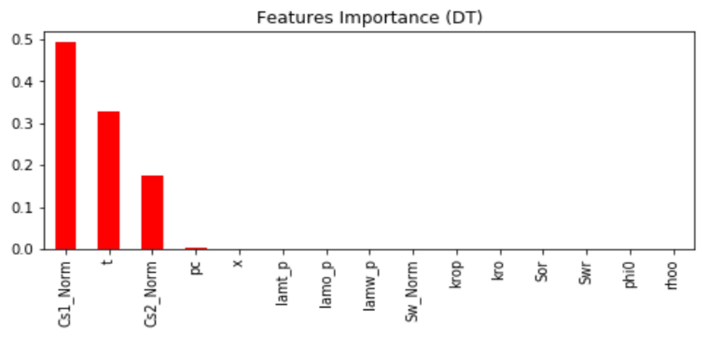
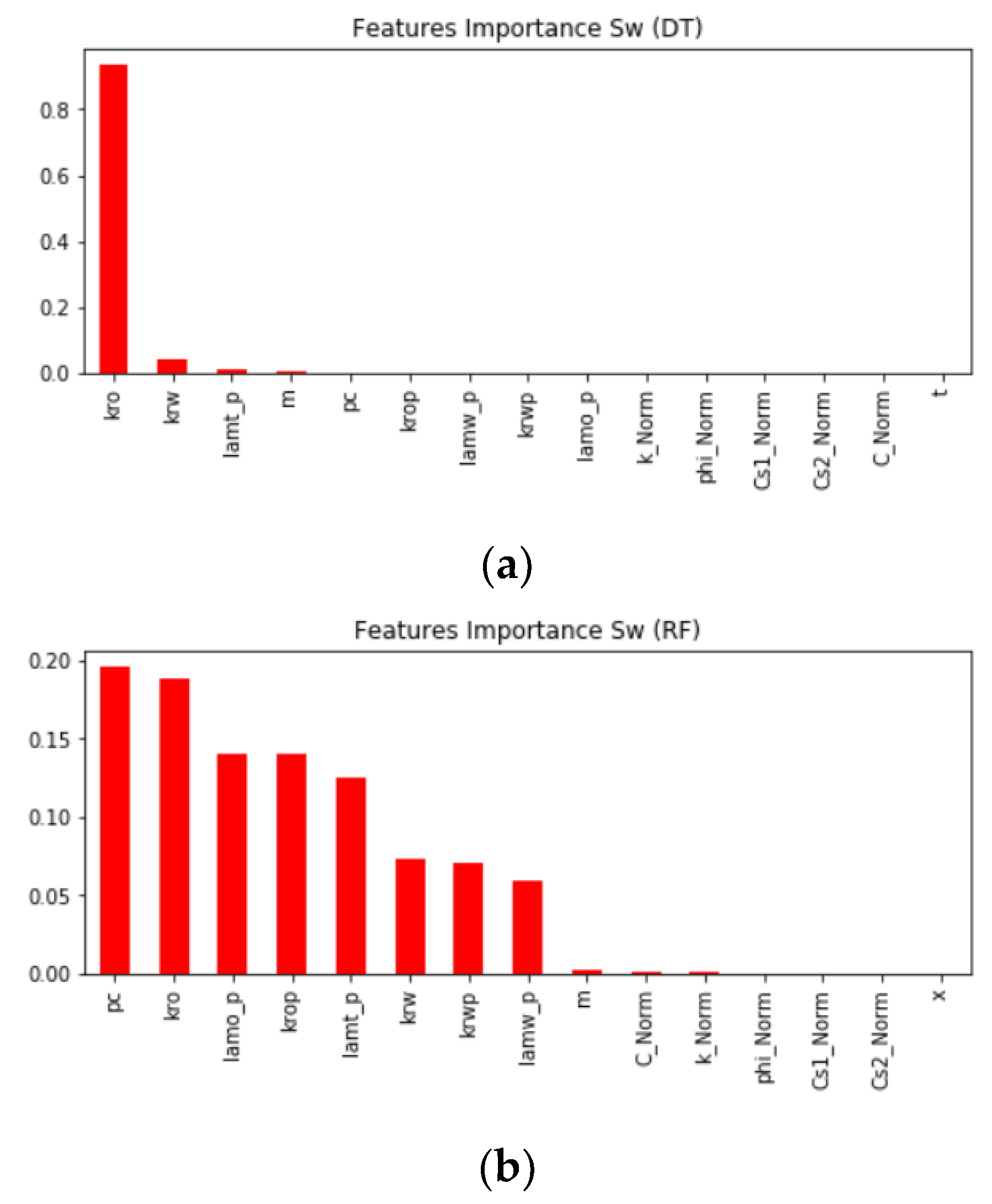
It was found out from most of the models tested that C_s1, C_s2, and t are the most important features that help in predicting the nanoparticles concentration. The score value calculated for each feature is varied from model to model. Figure 2 presents an example of the feature importance calculated for the DT model.

It can be seen in the feature importance figure that C_s1, t, and C_s2 are the most important features in predicting the nanoparticles concentration C. A comparative analysis between different machine learning models is provided, and it was found that the ANN model has the lowest root mean square error value of 0.000216 and the highest $R^2$ value of 0.999999, as shown in

Table 3. Model performance evaluation of two phases dataset for C.

Metric	RMSE	MSE	MAE	${\mathit{R}}^2$
DT	0.018360	0.000337	0.002237	0.995277
DT_sc *	0.018620	0.000347	0.002308	0.995142
RF	0.003747	0.000014	0.000232	0.999803
RF_sc *	0.004788	0.000023	0.000251	0.999679
GBR	0.027639	0.000764	0.008928	0.989297
GBR_sc *	0.001669	0.000003	0.001128	0.999961
ANN_ReLu_sc *	0.000216	0.000000	0.000202	0.999999

* sc: scaled dataset with standard scaler function.

.

In building the ANN model, we tried different numbers of hidden layers, different numbers of neurons, and different activation functions. We used three hidden layers with six neurons each, a rectifier activation function. Another model was built with three hidden layers of 15 neurons each and a rectifier activation function in the two hidden layers, and a sigmoid activation function in the output layer. We also build a third neural network with three hidden layers with six neurons, each with and rectifier activation function in two hidden layers and the third hidden layer with a tanh activation function. ReLu activation functions were found to perform better with an RMSE of 0.000216.

Table 4. Metric of ANN model with different activation functions for target C.

Metric	ANN (tanh)	ANN (sigmoid)	ANN (ReLu)
RMSE	0.000242	0.000566	0.000216
MSE	0.000000	0.000000	0.000000
MAE	0.000213	0.000446	0.000202
$R^2$	0.999999	0.999995	0.999999

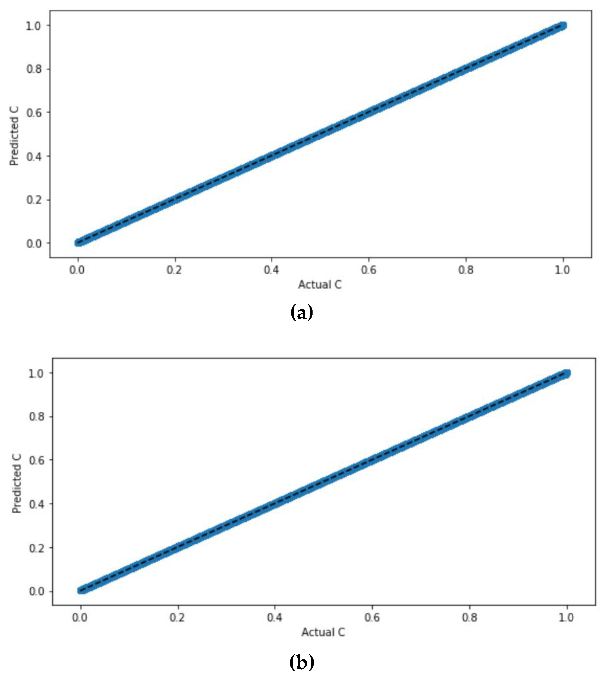
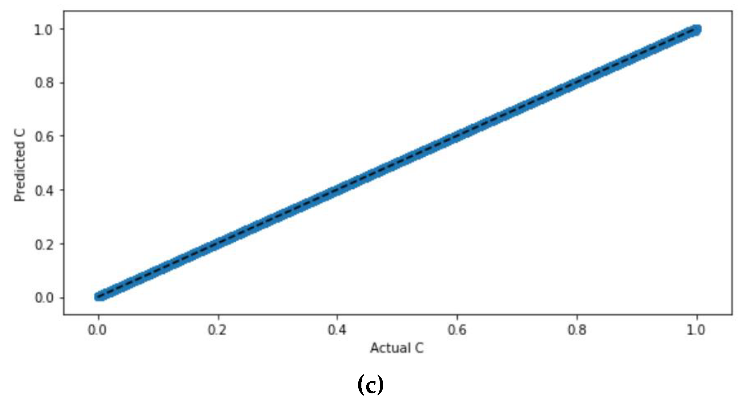
presents the evaluation of ANN models with different activation functions, and Figure 3 shows their scatter plots.

Figure 3 compares the scatter plots of the ANN model with the scaled dataset with ReLu, sigmoid, and tanh activation functions. It can be seen from the figure that the scatter plots of the ANN model with all the activation functions are similar with highly correlated values. The precise difference with regard to the accuracy values and error can be determined from the evaluation values listed in Table 4 that indicate that the ANN model with ReLu, sigmoid, and tanh activation functions, for the scaled dataset are all accurate with negligible differences.

We also checked the features’ importance for each model that predicts the nanoparticle concentrations, and we found out that each model selected different features. The most common features used are pc, k_rw, k_ro, lam_op, lam_wp, and lam_tp. The score value calculated for each feature is varied from model to model. Figure 4 demonstrates the feature importance in predicting S_w using DT, RF, and GBR models. It is shown from the figure that pc, k_rw, k_ro, k_rwp, k_rop, lam_wp, lam_op, lam_tp, and m are the most important features in most models.

Evaluating the models using different evaluation metrics, we found out that the ANN model with a standardized dataset and activation function of tanh performed the best in predicting the nanoparticles concentrations. ANN model had the lowest root mean square error value of 0.000125 and the highest $R^2$ value of 1.

Table 5. Models performance evaluation of two phases dataset for S_w.

Metric	RMSE	MSE	MAE	${\mathit{R}}^2$
DT	0.000235	0.000000	0.000039	0.999998
DT_sc *	0.000237	0.000000	0.000040	0.999998
RF	0.000212	0.000000	0.000022	0.999999
RF_sc *	0.000216	0.000000	0.000022	0.999999
GBR	0.000610	0.000000	0.000156	0.999989
GBR_sc *	0.000625	0.000000	0.000159	0.999989
ANN_tanh_sc *	0.000125	0.000000	0.000065	1.000000

* sc: scaled dataset.

presents the metric evaluation results of all models.

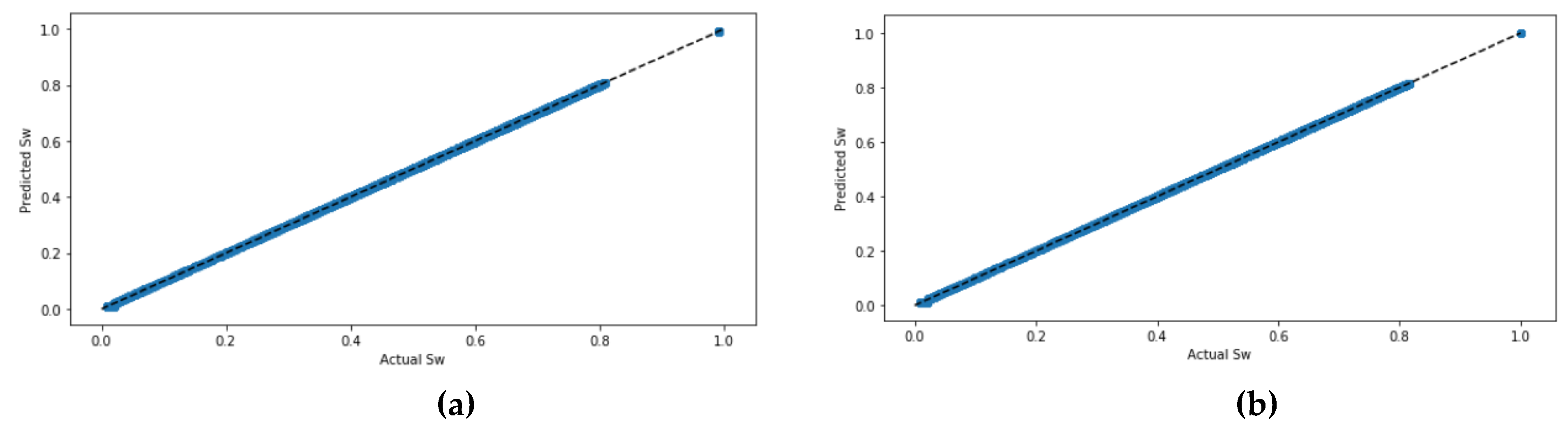
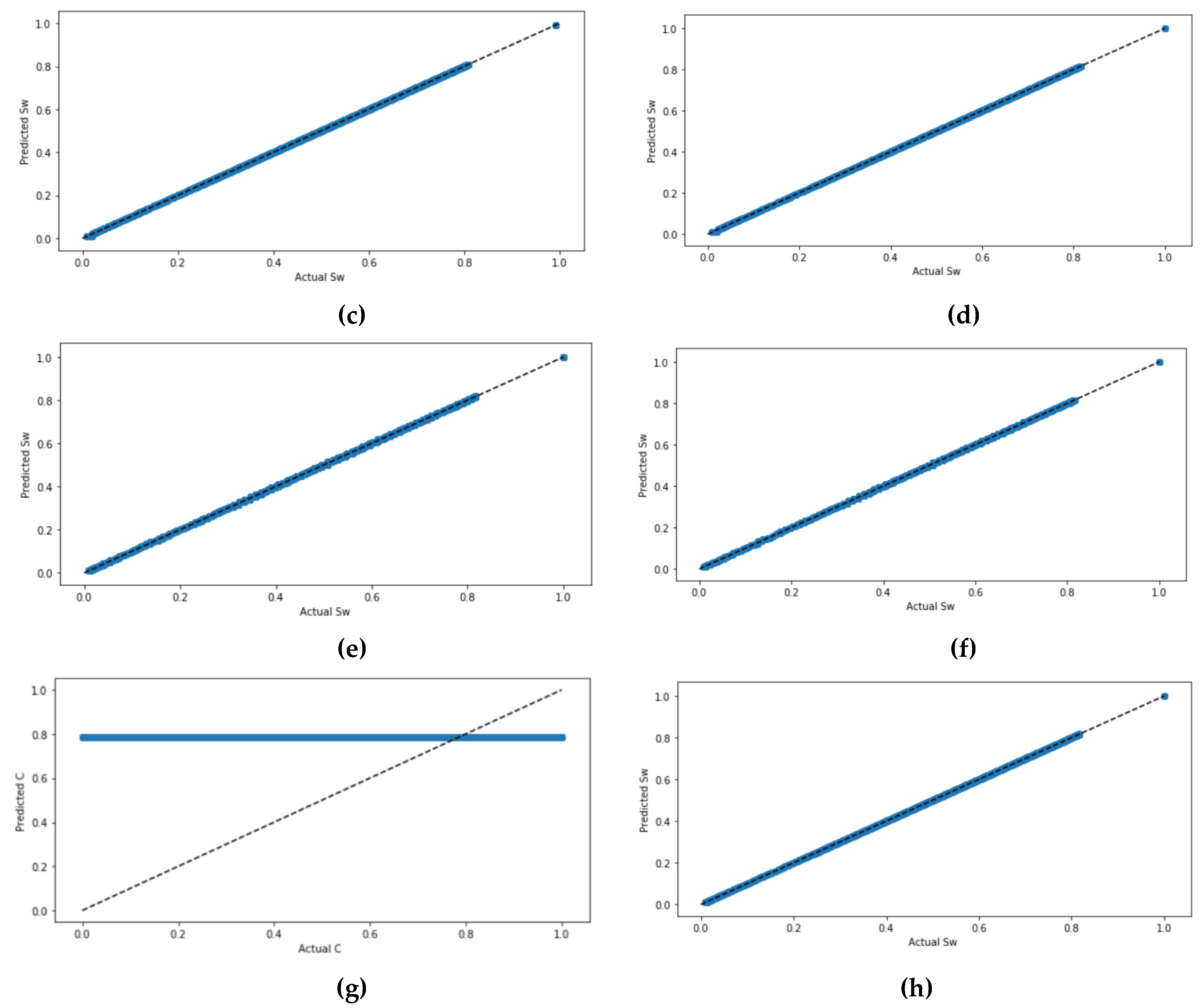
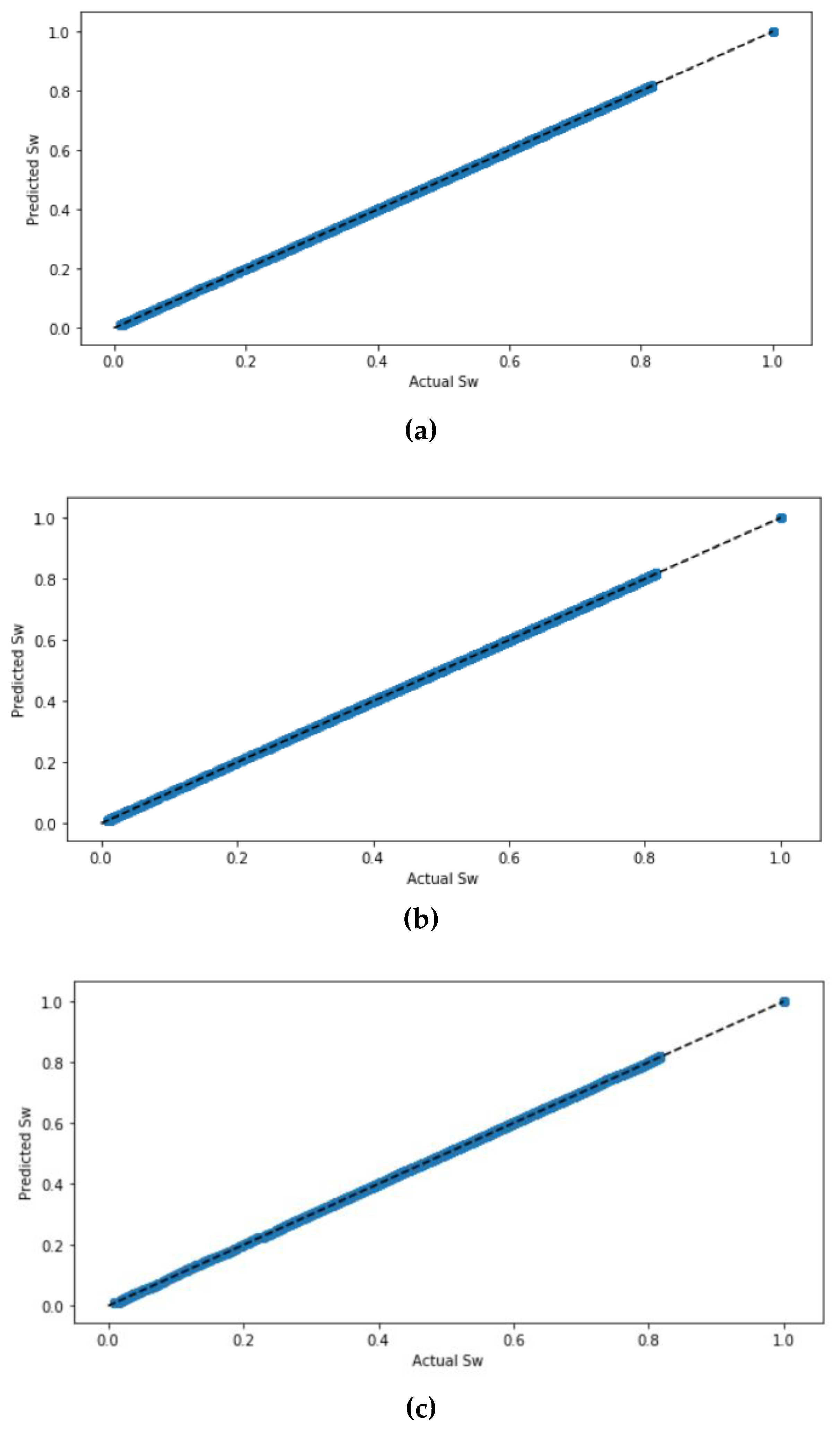
Figure 5 shows the actual values and the predicted values of S_w for all four ML models. The four models have been graphed twice: one time without scaling the datasets and the other time with scaling the dataset using the StandardScaler. It can be seen that predicting S_w when the dataset is not standardized had very close results to predicted values when the dataset became standardized, and the values in the figure are correlated. Except in the ANN model, which requires that the dataset standardize prior prediction. The ANN model with the tanh activation function had the highest correlated values in the scatter plot.

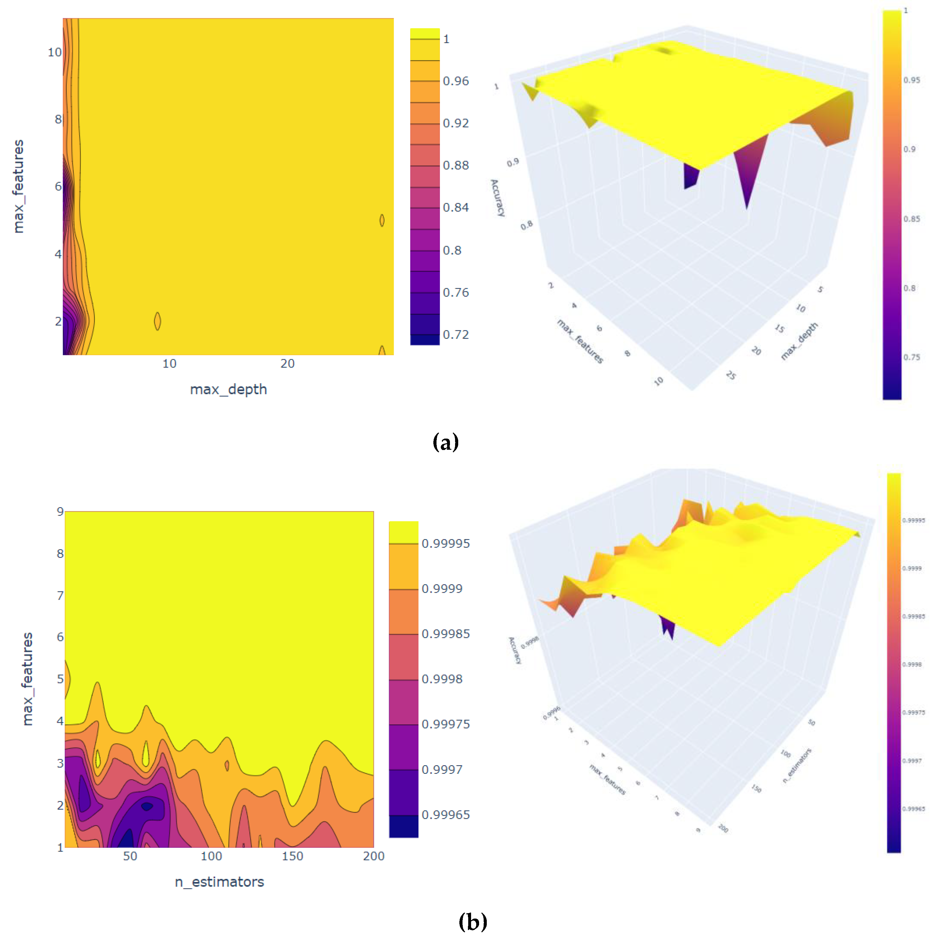
The model parameters are tuned to improve the performance of machine learning models. The hyperparameters, namely, max features and the number of estimators, are used. The 2D contour plot and the 3D surface plot of hyperparameter tuning are presented in Figure 6. The GridSearchCV was used for RF hyperparameters tuning, and it was found that the best parameters that would give the highest accuracy. For the DT model, the best parameter is a max depth of 19, and max feature of 9 would lead to an accuracy score of 1. When we scaled the data for training the GBR, the RMSE value (0.000605), and when training the model, the RMSE reduced further to reach (0.000292).

Moreover, different activation functions were used in three hidden layers with six neurons each, and we found out that “tanh” activation functions performed better.

Table 6. Evaluation metric of ANN models with different activation functions for target S_w.

Metric	ANN (tanh)	ANN (sigmoid)	ANN (ReLu)
RMSE	0.000125	0.000209	0.000310
MSE	0.000000	0.000000	0.000000
MAE	0.000065	0.000167	0.000083
$R^2$	1.000000	0.999999	0.999997

presents the evaluation of ANN models with different activation functions, and Figure 7 illustrates their scatter plots. Figure 7 compares the ANN model with the activation functions and shows that they are similar with highly correlated values. The accuracy and error can be determined from Table 5, which indicates that ANN with the tanh activation function had the lowest RMSE value and the highest R² value.

Now, let us discuss the results of predicting the oil relative permeability k_rop. First, we checked the features’ importance for each model when the target variable was k_rop, and we found out that each model selected different features. The most important feature found used in all models is lam_tp; other common features used by RF and GBR are pc, k_ro, and lam_op. The score value calculated for each feature is varied from model to model. Figure 8 presents the feature importance of the DT, RF, and GBR models. Figure 8 demonstrates the feature importance in predicting k_rop using DT, RF, and GBR models. It is shown from the figure that lam_tp, lam_op, pc, k_rw, k_ro, k_rwp, k_rop, lam_wp, and S_{w_Norm} are the most important features in most of the models.

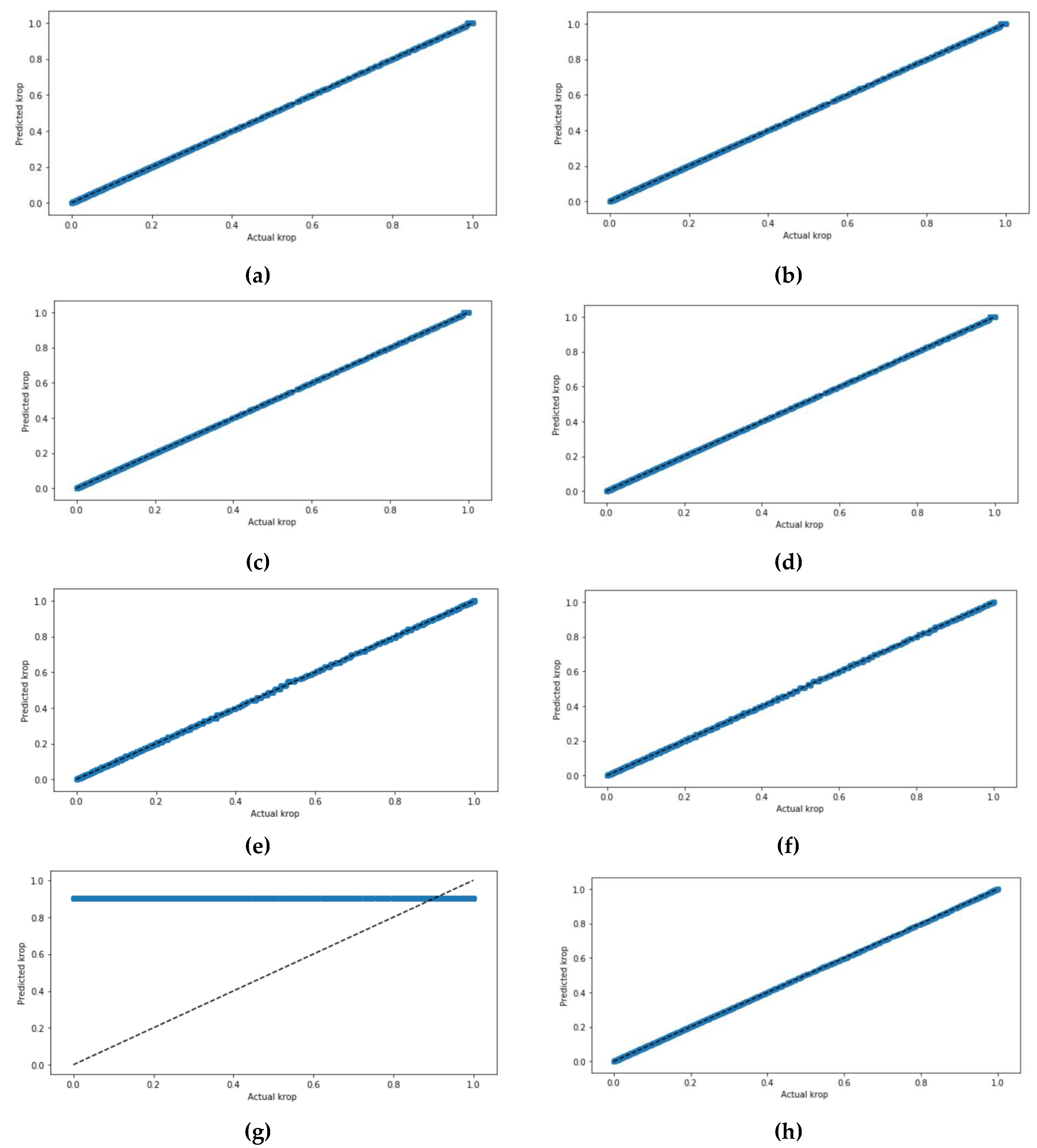
Evaluating the models using different evaluation metrics, we found out that most of the models tested have high performance when the target variable is k_rop, especially ANN models with standardized dataset and activation function of sigmoid that had RMSE value of 0.000145 and R² value of 1.000000. Figure 9 presents the scatterplot between the actual and the predicted k_rop.

Table 7. Models performance evaluation of two phases dataset for k_rop.

Metric	RMSE	MSE	MAE	${\mathit{R}}^2$
DT	0.000302	0.000000	0.000041	0.999999
DT_sc *	0.000303	0.000000	0.000041	0.999999
RF	0.000281	0.000000	0.000025	0.999999
RF_sc *	0.000280	0.000000	0.000026	0.999999
GBR	0.000442	0.000000	0.000088	0.999998
GBR_sc *	0.000423	0.000000	0.000087	0.999998
ANN_tanh_sc *	0.000182	0.000000	0.000047	1.000000
ANN_sigmoid_sc *	0.000145	0.000000	0.000115	1.000000
ANN_ReLu_sc *	0.000199	0.000000	0.000174	1.000000

* sc: scaled dataset.

presents the metric evaluation results of all models. Figure 9 demonstrates the actual values and predicted values of k_rop for all four models. It is shown that the scatter plots of all four models have a positive correlation. The scatter plots of each of the four models tested have been graphed twice, one time without scaling the datasets and the other time with scaling the dataset using the StandardScaler. Both scatter plots of each model that predict the k_rop had very close results when the dataset was standardized and not standardized in which the values in the figure are highly correlated, except in the ANN model, which requires that the dataset standardize prior prediction. The ANN model with the sigmoid activation function had the highest correlated values in the scatter plot.

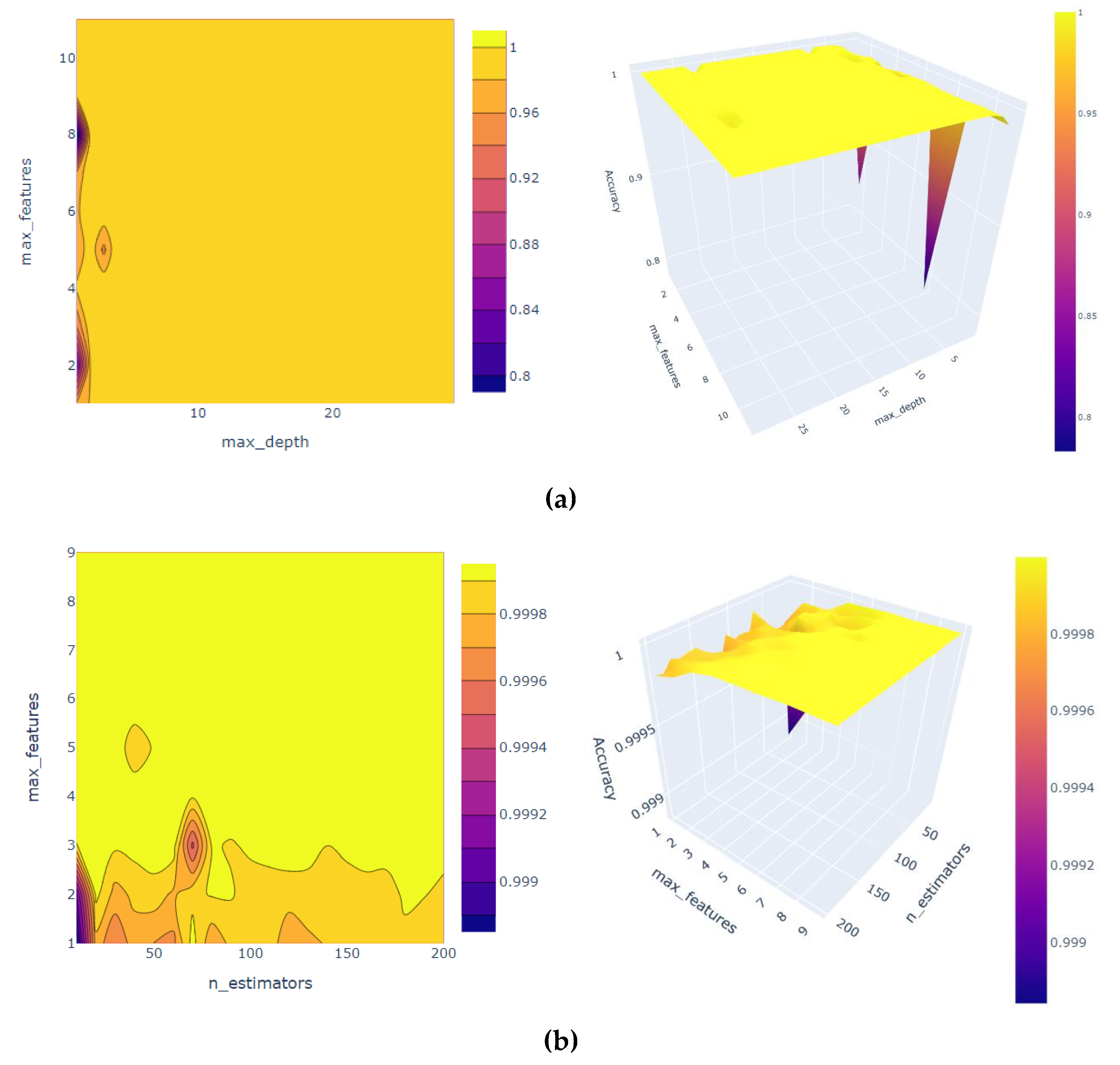
Most models when the target variable was k_rop had high performance without tuning the hyperparameters. The 2D contour and the 3D surface of the hyperparameter tuning of the RF model are shown in Figure 10. In the RF technique, the model provided good performance. Moreover, running the GridSearchCV function, we found out the best parameters are max-features of 9, and n-estimators of 40 would give an accuracy score of 1. Moreover, the DT model has a good performance without tuning, and when we run the GridSearchCV function, it provides an accuracy score of 1, a max-depth of 24, and a max-features of 8 would lead to an accuracy score of 1. The GBR model provided good performance in general. Therefore, we did not tune the hyperparameters.

Figure 10 illustrates the 2D contour and the 3D surface of tuning two hyperparameters using GridSearchCV for the relative permeability of oil k_rop when the medium surface is occupied with nanoparticles. Each 2D contour plot and 3D surface plot help to visualize the accuracy score of each two combinations of the selected hyperparameters in a color-coded manner. For the DT model, the two selected hyperparameters are max-depth and max-features. The yellow color code in both plots represents the highest accuracy score of 1 for both combinations when the max depth is 24, and the max features are 9. While for the RF model, the two selected hyperparameters are max-features and n-estimators. It is shown that max-features of 9 and n-estimators of 40 had the highest accuracy of a score of 1.

It is noteworthy that the difference between the results of DT and RF can be seen in the 3D surface. It is clear from Figure 6 and Figure 10 that the DT model’s accuracy is usually high for all values of the max-features parameter. However, for the RF model, the accuracy was lower with small values of the max-features parameter and increased quickly to reach high accuracy.

The ANN model with different activation functions provided high performance, especially with “tanh” activation functions (see

Table 8. Performance evaluation of the ANN model with different activation functions for the target k_rop.

Metric	ANN (tanh)	ANN (sigmoid)	ANN (ReLu)
RMSE	0.000182	0.000145	0.000199
MSE	0.000000	0.000000	0.000000
MAE	0.000047	0.000115	0.000174
$R^2$	1.000000	1.000000	1.000000

). Figure 11 compares the ANN prediction for a scaled dataset with ReLu, sigmoid, and tanh activation functions. It can be seen from the figure that the scatter plots of the ANN model with all the activation functions are similar with highly correlated values. The accuracy and error can be determined from the evaluation values listed in Table 8, which indicate that ANN with the sigmoid activation function had the lowest RMSE value.

This subsection presents the results of predicting k_rwp using DT, GBR, ANN, and RF algorithms. After evaluating all models, we found out that the RF model performed the best compared to other models. We checked the feature’s importance for each model when the target variable was k_rwp. The important features in most of the models are k_rw, k_ro, K, t, C_s1, C_s2, S_w, and pc. The score value calculated for each feature is varied from model to model. Figure 12 presents the feature importance of the DT, RF, and GBR models.

Figure 12. demonstrates the feature importance in predicting k_rwp using DT, RF, and GBR models. It is shown from the figure that t, S_{w_Norm}, C_{s1_Norm}, C_{s2_Norm}, pc, k_rw, and k_ro, are the most important features in most models.

We evaluated the models using different evaluation metrics and found that the RF model performed best when the target variable is k_rwp. The lowest RMSE value is 0.000281, and the highest R² value is 0.999999.

Table 9. Model performance evaluation of two phases dataset for k_rwp.

Metric	RMSE	MSE	MAE	${\mathit{R}}^2$
DT	0.000857	0.000001	0.000130	0.999989
DT_sc *	0.000877	0.000001	0.000130	0.999988
RF	0.000281	0.000000	0.000025	0.999999
RF_sc *	0.000581	0.000000	0.000053	0.999995
GBR	0.007716	0.000060	0.001552	0.999099
GBR_sc *	0.001261	0.000002	0.000270	0.999975
ANN_tanh_sc *	0.026346	0.000694	0.003855	0.989259
ANN_sigmoid_sc *	0.029402	0.000864	0.005519	0.986623
ANN_ReLu_sc *	0.036650	0.001343	0.005107	0.979215

* sc: scaled dataset.

presents the metric evaluation results of all models.

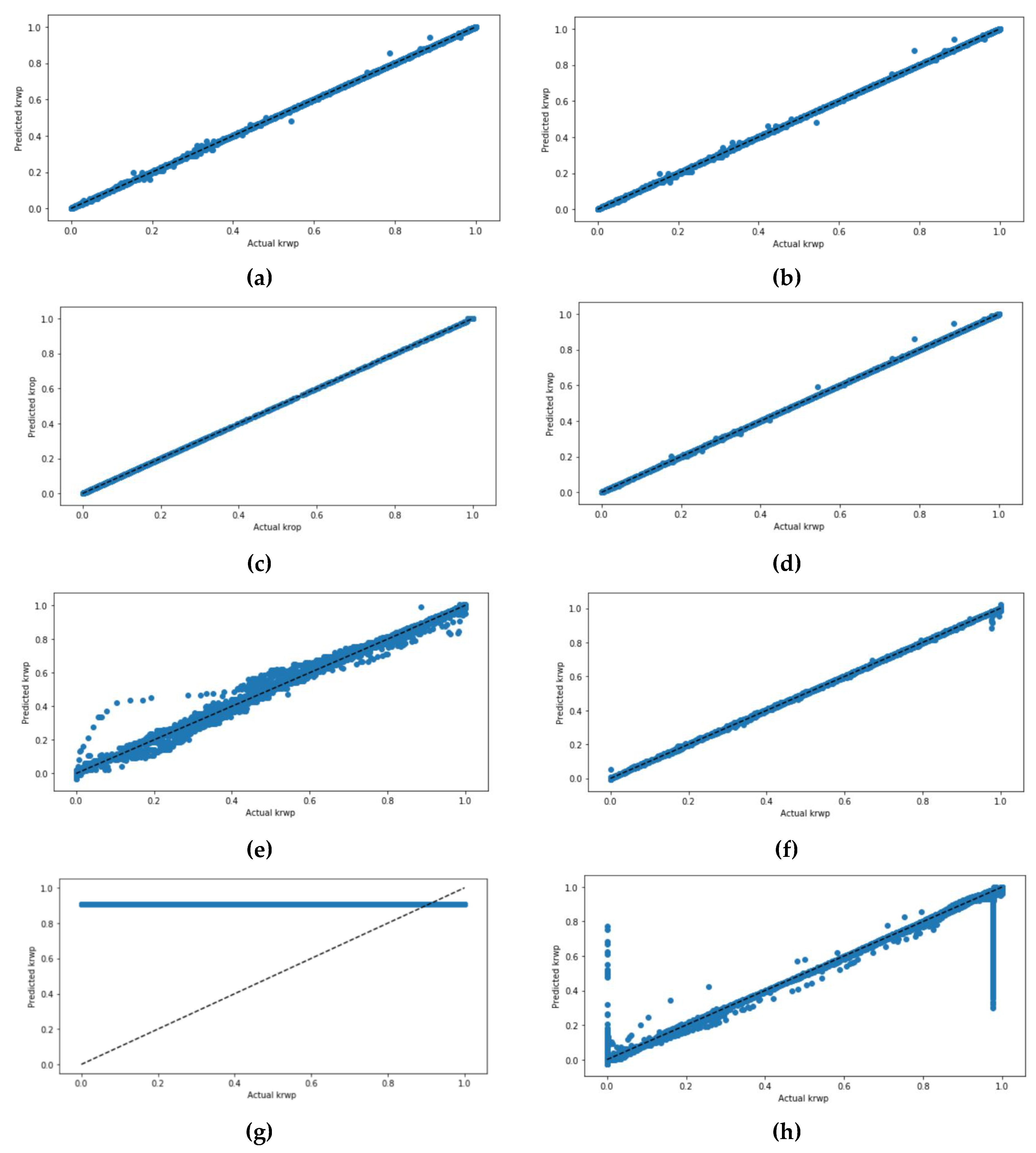
Figure 13 demonstrates the actual values and the predicted values of k_rwp for all four models. The scatter plots of all four models have been presented twice; one time without scaling the datasets and the other time with scaling the dataset using the StandardScaler. The DT model shows a minor difference between the scaled dataset and the not scaled dataset. The GBR model, when the dataset was not scaled, had some mispredicted values compared to the scaled dataset. Moreover, the ANN model with a scaled dataset also had some mispredicted values. At the same time, the RF model of the not scaled dataset had the highest correlated values compared to the other models.

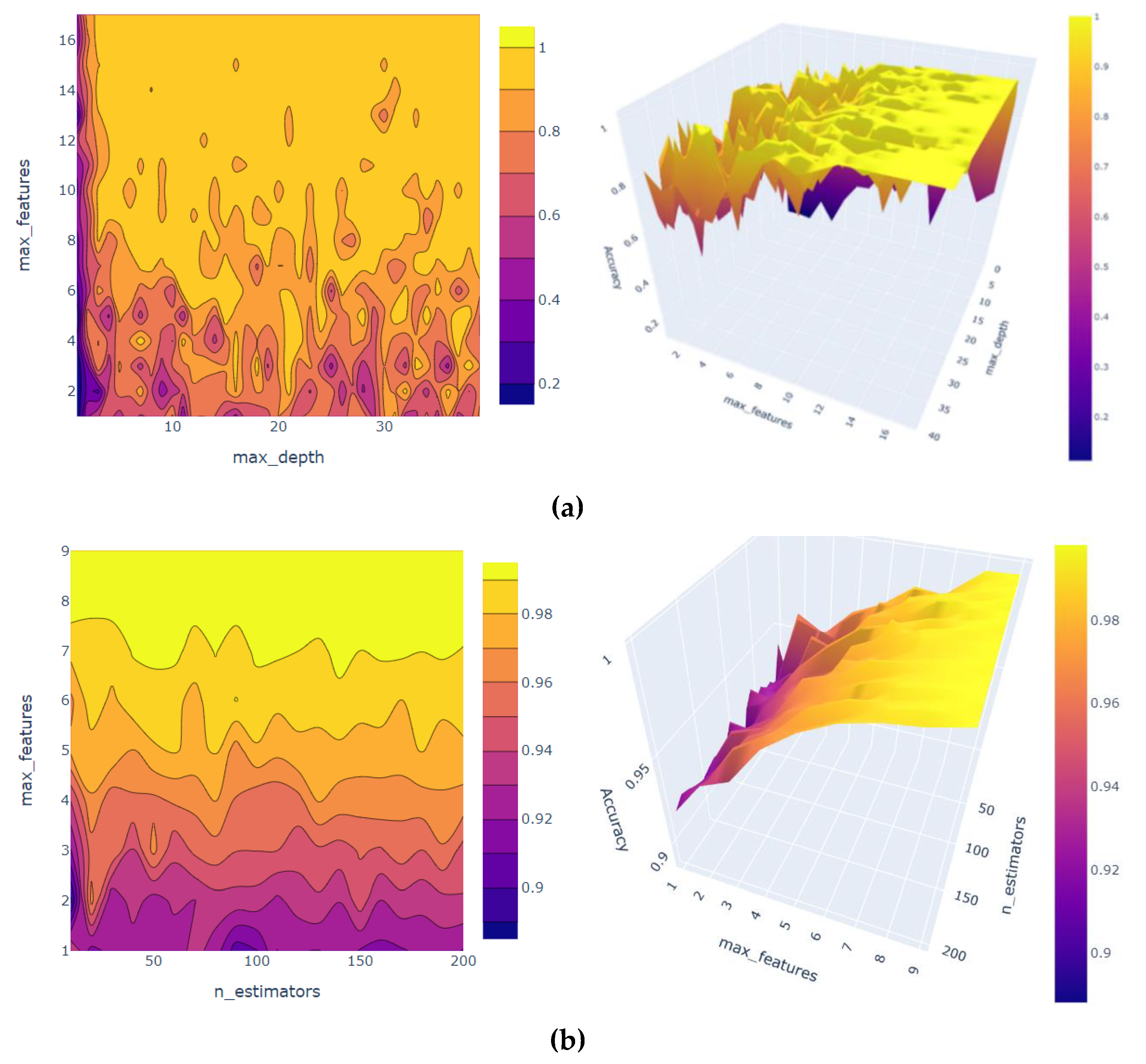
The performance of the model can be improved through hyperparameter tuning. In the RF technique, the model provided the highest performance compared to the other model. The 2D contour and the 3D surface of hyperparameter tuning are shown in Figure 14. The important features are presented in Figure 9 to train the RF model. Moreover, we ran the GridSerachCV function to check what parameters could give high accuracy. The best parameters of n-estimators of 60 and the max-features of 9 would provide an accuracy score of 1. A max-depth of 39 and max-features of 17 would lead to an accuracy score of 1. Comparing the GBR results with and without scaling, it was found that the scaled dataset would improve the model’s performance.

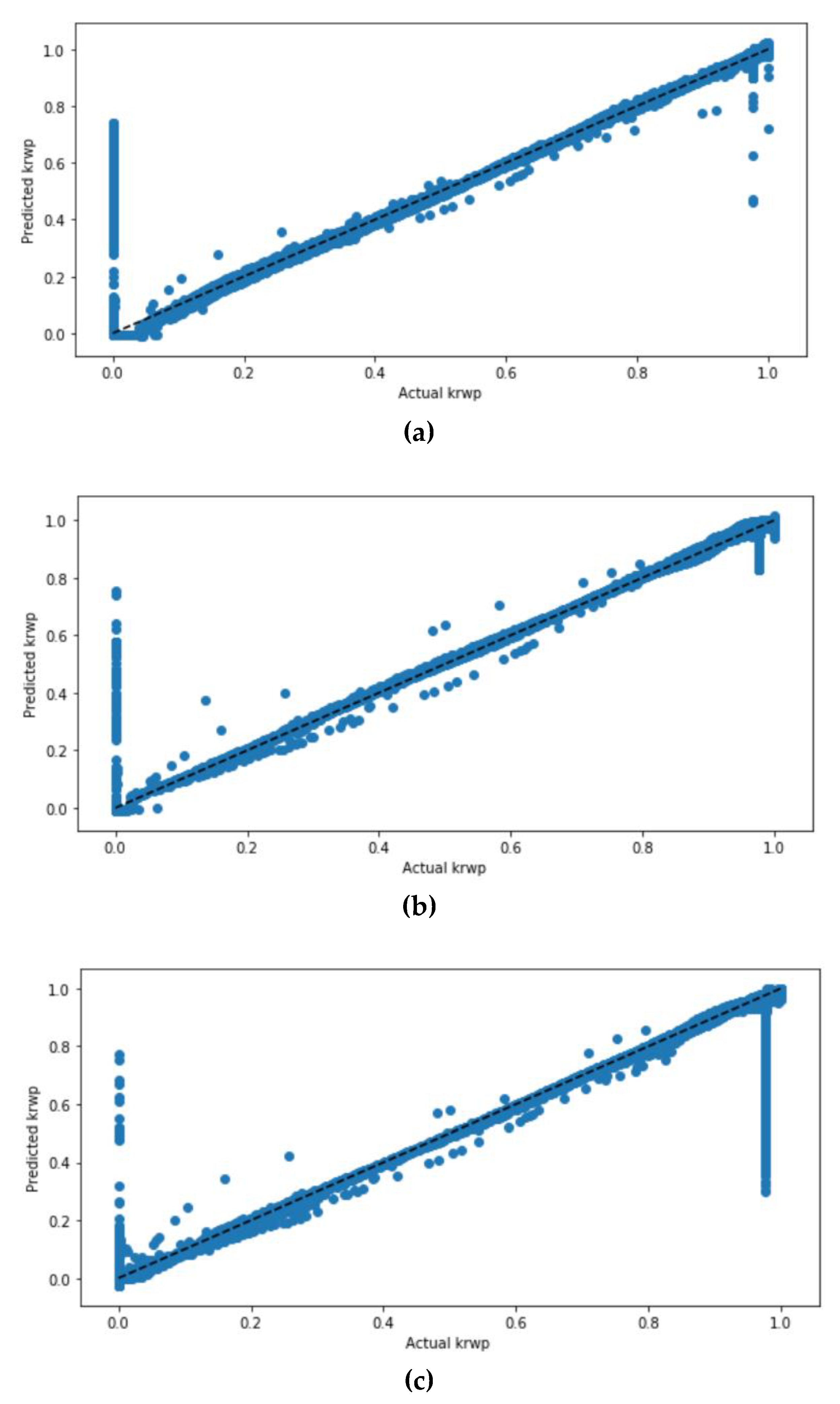
Three hidden layers have been used with the ANN models with six neurons each. The ReLu activation function has been used in two hidden layers, and the other activation functions have been used in the last hidden layer to monitor the performance of the model. It was found that the ANN model with the tanh activation function performed better (

Table 10. Performance evaluation metrics of the ANN model with different activation functions for the target k_rwp.

Metric	ANN (tanh)	ANN (sigmoid)	ANN (ReLu)
RMSE	0.026346	0.029402	0.036650
MSE	0.000694	0.000864	0.001343
MAE	0.003855	0.005519	0.005107
$R^2$	0.989259	0.986623	0.979215

and Figure 15). Figure 15 illuminates the 2D contour and the 3D surface of tuning two hyperparameters for the water relative permeability krwp. In the DT model, the two selected hyperparameters were the max-depth and max-features. It can be viewed from the figure that a max-depth of 39 and max-features of 17 had the highest accuracy score of 1. While for the RF model, the two selected hyperparameters are max-features and the number of estimators. It is shown that max-features of 9 and n-estimators of 60 had the highest accuracy of a score of 1.

Figure 15 compares the scatter plots of the ANN model with the scaled dataset with ReLu, sigmoid, and tanh activation functions. It can be seen from the figure that the scatter plots of the ANN model with the tanh activation function had the highest correlated values compared to the ANN model that used sigmoid and ReLu activation functions.

4. Conclusions

In this paper, machine learning techniques, including decision trees, random forests, gradient boosting regression, and artificial neural networks, were used to predict nanoparticle transport behavior in porous media. An artificial dataset has been generated for nanoparticle transport in two-phase flow modeled by the traditional mathematical continuum theory and validated against experimental results from the literature. The ML techniques were used to predict four target variables, including nanoparticle concentration, water saturation, and the relative permeability of oil and water. The scikit-learn library was used to investigate data preprocessing, correlation, and the feature importance of datasets, while the Standard scaler function was used to scale the datasets. Furthermore, the GridSearchCV algorithm was used to optimize hyperparameter tuning, and the ANN model was used with different activation functions. We evaluated the performance of the ML algorithms using four evaluation metrics: the mean absolute error, R-squared correlation, mean squared error, and root means squared error. It was found that the RF technique performed better in all four models when the target variable was k_rwp, while the ANN models performed better when the target variables were C, k_rop, and S_w. The features’ importance for each model has been determined, and it has been found that C_s1, C_s2, and t are the most important features that help predict the nanoparticle concentration. Moreover, the most commonly important features to predict water saturation are pc, k_rw, k_ro, lam_op, lam_wp, and lam_tp. Moreover, the model parameters are tuned to improve the performance of machine learning models and the hyperparameters, including max features and the number of estimators. The GridSearchCV was used for RF hyperparameter tuning. It was found that the best parameters would give the highest accuracy. For predicting S_w, the results of the non-scaled dataset were very close to the normalized dataset, while the opposite was true for the ANN model. The ANN model with ReLu, sigmoid, and tanh activation functions for the scaled dataset is all accurate with negligible differences.

References

1. Kong, X.; Ohadi, M.M. Applications of Micro and Nano Technologies in the Oil and Gas Industry-An Overview of the Recent Progress. In Proceedings of the Abu Dhabi International Petroleum Exhibition and Conference, Abu Dhabi, UAE, 1–4 November 2010. SPE-138241-MS. [Google Scholar]
2. Li, S. An Experimental Investigation of Enhanced Oil Recovery Mechanisms in Nanofluid Injection Process; Norwegian University of Science and Technology: Trondheim, Norway, 2016. [Google Scholar]
3. Yuan, B.; Wang, W.; Moghanloo, R.; Su, Y.; Wang, K.; Jiang, M. Permeability reduction of berea cores owing to nanoparticle adsorption onto the pore surface: Mechanistic modeling and expeimental work. Energy Fuels 2017, 31, 795–804. [Google Scholar] [CrossRef]
4. Kazemzadeh, Y.; Shojaei, S.; Riazi, M.; Sharifi, M. Review on application of nanoparticles for EOR purposes: A critical review of the opportunities and challenges. Chin. J. Chem. Eng. 2019, 27, 237–246. [Google Scholar] [CrossRef]
5. Sabet, M.; Hosseini, S.; Zamani, A.; Hosseini, Z.; Soleimani, H. Application of nanotechnology for enhanced oil recovery: A review. Defect Diffus. Forum 2016, 367, 149–156. [Google Scholar] [CrossRef]
6. Tiab, D.; Donaldson, E.C. Petrophysics: Theory; Practice of Measuring Reservoir Rock; Fluid Transport Properties; Gulf Professional Publishing: Houston, TX, USA, 2015. [Google Scholar]
7. Lashari, N.; Ganat, T. Emerging applications of NANOMATERIALS in chemical enhanced oil recovery: Progress and perspective. Chin. J. Chem. Eng. 2020, 8, 1995–2009. [Google Scholar] [CrossRef]
8. Aghajanzadeh, M.R.; Ahmadi, P.; Sharifi, M.; Riazi, M. Wettability modification of oil-wet carbonate reservoirs using silica-based nanofluid: An experimental approach. J. Pet. Sci. Eng. 2019, 178, 700–710. [Google Scholar] [CrossRef]
9. Maghzi, A.; Kharrat, R.; Mohebbi, A.; Ghazanfari, M.H. The impact of silica nanoparticles on the performance of polymer solution in presence of salts in polymer flooding for heavy oil recovery. Fuel 2014, 123, 123–132. [Google Scholar] [CrossRef]
10. Wasan, D.T.; Nikolov, A.D. Spreading of nanofluids on solids. Nature 2003, 423, 156–159. [Google Scholar] [CrossRef]
11. Ju, B.; Fan, T. Experimental study and mathematical model of nanoparticle transport in porous media. Powder Technol. 2009, 192, 195–202. [Google Scholar] [CrossRef]
12. Youssif, M.I.; El-Maghraby, R.M.; Saleh, S.M.; Elgibaly, A. Silica nanofluid flooding for enhanced oil recovery in sandstone rocks. Egypt. J. Pet. 2018, 27, 105–110. [Google Scholar] [CrossRef]
13. Khalilinezhad, S.S.; Cheraghian, G.; Karambeigi, M.; Tabatabaee, H.; Roayaei, E. Characterizing the role of clay and silica nanoparticles in enhanced heavy oil recovery during polymer flooding. Arab. J. Sci. Eng. 2016, 41, 2731–2750. [Google Scholar] [CrossRef]
14. Khalilinezhad, S.S.; Cheraghian, G.; Roayaei, E.; Tabatabaee, H.; Karambeigi, M.S. Improving heavy oil recovery in the polymer flooding process by utilizing hydrophilic silica nanoparticles. Energy Sources Part A Recovery Util. Environ. Eff. 2017, 1–10. [Google Scholar] [CrossRef]
15. Jeong, S.-W.; Kim, S.-D. Aggregation and transport of copper oxide nanoparticles in porous media. J. Environ. Monit. 2009, 11, 1595–1600. [Google Scholar] [CrossRef] [PubMed]
16. Shafiq, A.; Mebarek-Oudina, F.; Sindhu, T.N.; Rassoul, G. Sensitivity analysis for Walters’ B nanoliquid flow over a radiative Riga surface by RSM. Scientia Iranica 2022, 29, 1236–1249. [Google Scholar]
17. El-Amin, M.F.; Sun, S.; Salama, A. Enhanced oil recovery by nanoparticles injection: Modeling and simulation. In Proceedings of the SPE Middle East Oil and Gas Show and Conference, Manama, Bahrain, 10–13 March 2013. SPE-164333-MS. [Google Scholar]
18. El-Amin, M.; Salama, A.; Sun, S. Numerical and dimensional analysis of nanoparticles transport with two-phase flow in porous media. J. Pet. Sci. Eng. 2015, 128, 53–64. [Google Scholar] [CrossRef]
19. Zhang, X.-D. Machine learning. In A Matrix Algebra Approach to Artificial Intelligence; Springer: Berlin/Heidelberg, Germany, 2020; pp. 223–440. [Google Scholar]
20. Pirizadeh, M.; Alemohammad, N.; Manthouri, M.; Pirizadeh, M. A new machine learning ensemble model for class imbalance problem of screening enhanced oil recovery methods. J. Pet. Sci. Eng. 2021, 198, 108214. [Google Scholar] [CrossRef]
21. Daribayev, B.; Akhmed-Zaki, D.; Imankulov, T.; Nurakhov, Y.; Kenzhebek, Y. Using Machine Learning Methods for Oil Recovery Prediction. In ECMOR XVII; European Association of Geoscientists & Engineers: Bunnik, The Netherlands, 2020; pp. 1–13. [Google Scholar]
22. Esfe, M.H.; Bahiraei, M.; Mahian, O. Experimental study for developing an accurate model to predict viscosity of CuO–ethylene glycol nanofluid using genetic algorithm based neural network. Powder Technol. 2018, 338, 383–390. [Google Scholar] [CrossRef]
23. Changdar, S.; Saha, S.; De, S. A smart model for prediction of viscosity of nanofluids using deep learning. Smart Sci. 2020, 8, 242–256. [Google Scholar] [CrossRef]
24. Subasi, A.; El-Amin, M.; Darwich, T.; Dossary, M. Permeability prediction of petroleum reservoirs using stochastic gradient boosting regression. J. Ambient. Intell. Humaniz. Comput. 2020, 13, 3555–3564. [Google Scholar] [CrossRef]
25. Zhou, K.; Li, S.; Zhou, X.; Hu, Y.; Zhang, C.; Liu, J. Data-driven prediction and analysis method for nanoparticle transport behavior in porous media. Measurement 2021, 172, 108869. [Google Scholar] [CrossRef]
26. Goldberg, E.; Scheringer, M.; Bucheli, T.D.; Hungerbühler, K. Prediction of nanoparticle transport behavior from physicochemical properties: Machine learning provides insights to guide the next generation of transport models. Environ. Sci. Nano 2015, 2, 352–360. [Google Scholar] [CrossRef] [Green Version]
27. Irfan, S.A.; Shafie, A. Artificial Neural Network Modeling of Nanoparticles Assisted Enhanced Oil Recovery. In Advanced Methods for Processing and Visualizing the Renewable Energy; Springer: Berlin/Heidelberg, Germany, 2021; pp. 59–75. [Google Scholar]
28. Kotsiantis, S.B. Decision trees: A recent overview. Artif. Intell. Rev. 2013, 39, 261–283. [Google Scholar] [CrossRef]
29. Breiman, L. Random Forests. Mach. Learn. 2001, 45, 5–32. [Google Scholar] [CrossRef] [Green Version]
30. El-Amin, M.F.; Subasi, A. Forecasting a Small-Scale Hydrogen Leakage in Air using Machine Learning Techniques. In Proceedings of the 2020 2nd International Conference on Computer and Information Sciences (ICCIS), Sakaka, Saudi Arabia, 13–15 October 2020; pp. 1–5. [Google Scholar]
31. Alwated, B.; El-Amin, M.F. Enhanced oil recovery by nanoparticles flooding: From numerical modeling improvement to machine learning prediction. Adv. Geo. Energy Res. 2021, 5, 297–317. [Google Scholar] [CrossRef]
32. Zhang, Y.; Haghani, A. A gradient boosting method to improve travel time prediction. Transp. Res. Part C Emerg. Technol. 2015, 58, 308–324. [Google Scholar] [CrossRef]
33. del Castillo, A.Á.; Santoyo, E.; García-Valladares, O. A new void fraction correlation inferred from artificial neural networks for modeling two-phase flows in geothermal wells. Comput. Geosci. 2012, 41, 25–39. [Google Scholar] [CrossRef]
34. Lippmann, R. An introduction to computing with neural nets. IEEE Assp Mag. 1987, 4, 4–22. [Google Scholar] [CrossRef]
35. Hansen, L.K.; Salamon, P. Neural network ensembles. IEEE Trans. Pattern Anal. Mach. Intell. 1990, 12, 993–1001. [Google Scholar] [CrossRef] [Green Version]
36. Sahli, H. An introduction to machine learning. In TORUS 1–Toward an Open Resource Using Services: Cloud Computing for Environmental Data; Wiley: Hoboken, NJ, USA, 2020; pp. 61–74. [Google Scholar]
37. Mohaghegh, S.; Ameri, S. Artificial Neural Network as a Valuable Tool for Petroleum Engineers. In SPE Paper 29220; SPE: Bridgeport, WV, USA, 1995. [Google Scholar]
38. El-Amin, M.F.; Subasi, A. Predicting Turbulent Buoyant Jet Using Machine Learning Techniques. In Proceedings of the 2020 2nd International Conference on Computer and Information Sciences (ICCIS), Sakaka, Saudi Arabia, 13–15 October 2020; pp. 1–5. [Google Scholar]
39. El-Amin, M.F.; Kou, J.; Sun, S. Convergence analysis of the nonlinear iterative method for two-phase flow in porous media associated with nanoparticle injection. Int. J. Num. Meth. Heat Fluid Flow 2017, 27, 2289–2317. [Google Scholar] [CrossRef]
40. Ju, B.; Dai, S.; Luan, Z.; Zhu, T.; Su, X.; Qiu, X. A study of wettability and permeability change caused by adsorption of nanometer structured polysilicon on the surface of porous media. In Proceedings of the SPE Asia Pacific Oil and Gas Conference and Exhibition, Melbourne, Australia, 8–10 October 2002. [Google Scholar]
41. Skjaeveland, S.; Siqveland, L.; Kjosavik, A.; Thomas, W.; Virnovsky, G. Capillary pressure correlation for mixed-wet reservoirs. SPE Reserv. Eval. Eng. 2000, 3, 60–67. [Google Scholar] [CrossRef]
Figure 1. Nanoparticle behaviors against pore volume. (a) Nanoparticles concentration, (b) Water saturation.
Energies 16 00678 g001
Figure 2. Features importance of DT for predicting C.
Energies 16 00678 g002
Figure 3. Scatter plots of ANN models with different activation functions (a) “ReLu” activation function, (b) “sigmoid” activation function, and (c) “tanh” activation function, for target C. The dashed line represents a full coinciding between actual and predicted data.
Energies 16 00678 g003aEnergies 16 00678 g003b
Figure 4. Features importance of (a) DT, (b) RF, and (c) GBR models for predicting Sw.
Energies 16 00678 g004aEnergies 16 00678 g004b
Figure 5. Actual vs. predicted water saturation using machine learning techniques DT, RF, GBR, and ANN for Sw. (a) DT without scaling, (b) DT with scaling, (c) RF without scaling, (d) RF with scaling, (e) GBR without scaling, (g) GBR with scaling, (f) ANN without scaling with tanh, (h) ANN scaling with tanh. The dashed line represents a full coinciding between actual and predicted data.
Energies 16 00678 g005aEnergies 16 00678 g005b
Figure 6. 2D contour and 3D surface plots of hyperparameters tuning for (a) DT, and (b) RF for target Sw.
Energies 16 00678 g006
Figure 7. Scatter plots of ANN models with different activation functions (a) “ReLu” activation function, (b) “sigmoid” activation function, and (c) “tanh” activation function, for target Sw. The dashed line represents a full coinciding between actual and predicted data.
Energies 16 00678 g007
Figure 8. Features importance of (a) DT, (b) RF, and (c) GBR models for predicting krop.
Energies 16 00678 g008
Figure 9. Actual against predicted krop using different machine learning techniques DT, RF, GBR, and ANN. (a) DT without scaling, (b) DT with scaling, (c) RF without scaling, (d) RF with scaling, (e) GBR without scaling, (g) GBR with scaling, (f) ANN without scaling with tanh, (h) ANN scaling with tanh. The dashed line represents a full coinciding between actual and predicted data.
Energies 16 00678 g009
Figure 10. 2D contour and the 3D surface of hyperparameters tuning for (a) DT, and (b) RF for the target krop.
Energies 16 00678 g010
Figure 11. ANN prediction with different activation functions (a) “ReLu” activation function, (b) “sigmoid” activation function, and (c) “tanh” activation function, for the target krop. The dashed line represents a full coinciding between actual and predicted data.
Energies 16 00678 g011
Figure 12. Features importance of (a) DT, (b) RF, and (c) GBR models for predicting krwp.
Energies 16 00678 g012
Figure 13. Actual vs. predicted krwp using different machine learning techniques DT, RF, GBR, and ANN. (a) DT without scaling, (b) DT with scaling, (c) RF without scaling, (d) RF with scaling, (e) GBR without scaling, (g) GBR with scaling, (f) ANN without scaling with tanh, (h) ANN scaling with tanh. The dashed line represents a full coinciding between actual and predicted data.
Energies 16 00678 g013
Figure 14. 2D contour and the 3D surface of hyperparameters tuning for (a) DT, and (b) RF for the target krwp.
Energies 16 00678 g014
Figure 15. ANN predictions with different activation functions (a) “ReLu” activation function, (b) “sigmoid” activation function, and (c) “tanh” activation function, for the target krwp. The dashed line represents a full coinciding between actual and predicted data.
Energies 16 00678 g015