Abstract
A permanent magnet synchronous motor (PMSM) is a crucial device for power conversion in an energy system. The cogging torque of the PMSM is a crucial output characteristic, the robustness of which affects the operational reliability of the energy system. Therefore, the robust design optimization (RDO) of cogging torque has aroused widespread concern. There are several challenges in designing a robust cogging torque PMSM. In particular, some design parameters contain repetitive units, and the finite element analysis (FEA) method is time-consuming. State-of-the-art RDO methods usually treat these uncertainties from repetitive units as the same parameter, which neglects the fluctuation of the manufacturing process and cannot obtain a robust solution for the cogging torque of the motor efficiently and accurately. In order to solve this issue, an approximate modeling method based on manufacturing uncertainties analysis for RDO is proposed in this paper. First, the peak-to-peak value of cogging torque (Tcpp) is used to characterize the cogging torque, which is decoupled to an ideal component and fluctuation component produced by the center values and manufacturing tolerances of design parameters. The design of experiments (DoE) and simulation of the two components are carried out. Then, these two components are approximated separately, and the approximate model of Tcpp is obtained by adding the two components. Finally, the proposed approximate model is embedded into the RDO algorithm, and the PMSM design scheme for good Tcpp robustness is obtained. The effectiveness of the proposed method is verified through a case study of the PMSM.
1. Introduction
With more rigorous demands for energy saving and environmental protection in the industry, mechanical arms and new energy-electric vehicles driven by electric motors are being widely developed [1]. Permanent magnet synchronous motors (PMSMs), which present high efficiency and low torque ripple [2,3], are commonly applied to high-precision servo equipment in the environmental energy industry, such as precision rotary tables, robots, CNC machines, new energy electric vehicles [4,5] (the leading applications are shown in Figure 1). Compared with other motors, PMSM has a relatively low torque ripple. Low torque ripple cannot be ignored in high-precision applications, such as robot elbow joints and CNC machines, which have high requirements for control accuracy and positioning accuracy. Pursuing lower torque ripple is still a research hotspot in motor optimization. The cogging torque of the PMSM is the inherent torque generated by the motor’s interaction between the stator and rotor. It also exists even in an ideal situation. The cogging torque produces the torque ripple, which reduces the positioning accuracy and control accuracy and limits the application of the PMSM in high-precision cases. The peak-to-peak value of the cogging torque (Tcpp) is used to quantify this fluctuation. As the PMSM has repetitive units affected by manufacturing uncertainties, the inconsistency of the Tcpp of a batch of motors significantly impacts the quality, reliability, performance, and cost of the servo equipment [6]. Therefore, with existing manufacturing accuracy, reducing the Tcpp in a batch of motors and improving its overall robustness is an important and challenging task.
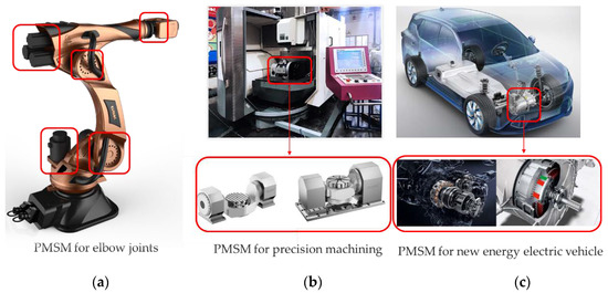
Figure 1.
Typical applications of permanent magnet synchronous motors in the environmental energy industry: (a) robots; (b) high-precision servo equipment; (c) new energy electric vehicles.
In order to improve the product quality in a batch of motors, many scholars have adopted robust design optimization (RDO) [7,8] to improve the robustness of Tcpp. RDO refers to finding the design that makes the output response least sensitive to noise with the existing manufacturing uncertainties. Many scholars have introduced RDO into the optimization of motor efficiency, controllers, vibration, and Tcpp, and most of these research activities are based on finite element analysis (FEA). However, the conventional RDO methods using electromagnetic simulations are usually based on symmetry models in which these uncertainties of permanent magnets and stator slots from repetitive units are treated as a single random variable. They deal with different design variables or parameters as a single uncertainty. It is necessary to utilize a complete model due to the combined effect of the uncertainties caused by repetitive units being different from that of a single variable [9]. The FEA is time-consuming because the RDO process requires many iterative simulations. Therefore, an approximate model is proposed to replace the FEA to improve the optimization process efficiency. Some scholars have adopted Kriging [10], support vector machines (SVMs) [11], and the response surface model [12] for RDO. When considering the manufacturing uncertainties, the number of samples required by the conventional approximate modeling method increases sharply with the increase in design parameters, which brings apparent limitations to the approximate modeling of Tcpp. Lee and Kim et al. establish an approximate model of output response using analytical methods but only focus on optimizing a single design parameter when considering the manufacturing uncertainties of repetitive units [13,14,15]. However, the relationship between various design parameters and the Tcpp is nonlinear. Thus, multi-parameter or global optimization of the motor is not equivalent to the superposition of individual single-parameter optimizations. Therefore, the optimal global solution cannot be obtained by optimizing a single parameter, which is not suitable for the design process of multiple design parameters.
In order to solve the above problems, we propose an RDO method based on approximate modeling considering manufacturing uncertainties, in which the approximate modeling is based on the traditional approximate modeling without considering the uncertainty, supplemented with the approximate modeling of the fluctuation component caused by the uncertainties. The two parts of the model are added together to obtain the approximate model considering the uncertainties. The approximate model is applied to the RDO process. Firstly, to decouple the effect of the center values and the manufacturing uncertainties of the design parameters on the Tcpp, we divide the Tcpp into the ideal component dominated by the center values of the design parameters and the fluctuation component jointly affected by the manufacturing uncertainties. The two components are sampled and modeled separately. Then, an approximate model is conducted separately for the two components. The relationship between the center values and the ideal component of Tcpp is the model without considering uncertainties, so it can be directly modeled by using the conventional approximate modeling method. As the theoretical analysis shows that the fluctuation component is related to the center values and manufacturing uncertainties [9,16,17,18], the fluctuation component can be approximately obtained by the manufacturing deviation rates. The manufacturing deviation rate is the ratio of the manufacturing deviation and center values. The higher the dimension of the manufacturing deviation of repetitive units, the higher the approximate complexity. Therefore, when the training samples are relatively limited, the random forest (RF) was used to model the fluctuation component. On the one hand, the bagging method was used to expand the number of training samples; On the other hand, the relationship between the manufacturing deviation rates of parameters and the fluctuation component of Tcpp is trained by decision trees. The output of the fluctuation component model is added to the output of the ideal component model, and the Tcpp considering manufacturing uncertainties is obtained. Finally, the proposed approximate model is applied to the RDO of the PMSM to reduce the mean and standard deviation of the motors’ Tcpp, verifying the scheme’s effectiveness.
The critical aspects of the approximate modeling method for RDO proposed in this paper are as follows: first, the approximate model of the ideal components of Tcpp is comparable to the conventional approximate model without considering the tolerances, which requires a small number of samples, while the traditional approximate modeling method can be used to obtain more accurate approximate results. Second, the complementary modeling of the fluctuation component of Tcpp is used to compensate for components caused by manufacturing deviations of repetitive units that are not considered in the ideal component model. As a result, the accuracy of the overall approximate model is improved.
The rest of the paper is organized as follows: Section 2 introduces the proposed approach’s overall thought and basic flow. A parametric FEA is established to extract the training database of the approximate modeling, and the key parameters are screened to reduce the approximate modeling dimension. An approximate modeling method considering the uncertainties of repetitive units is proposed for RDO. Then, the RDO method is proposed. Section 3 takes a PMSM as an example, demonstrating the superiority of the proposed approximate modeling. The robust optimization results can be obtained when the approximate modeling is applied to RDO. Section 4 conveys the concluding remarks.
2. The Proposed RDO Approach Considering Manufacturing Uncertainties of the PMSM
In the actual production process of the PMSM, there are inevitable manufacturing uncertainties because the structure of the PMSM has repetitive units, and the uncertainty of a single design parameter comes from multiple units. The traditional RDO needs to consider this issue, and the optimization scheme obtained is insignificant in actual production. In order to solve this problem, the uncertainties of repetitive units caused by manufacturing uncertainties are fully considered in the RDO process for the PMSM. In order to take into account the calculation accuracy and efficiency of the RDO, an approximate model considering the uncertainties of the actual manufacturing process was established to replace the FEA. Therefore, the actual machining parameters of the PMSM need to be accurately analyzed by FEA first, from which the training data with the actual production conditions were extracted for approximate modeling. In Section 2.2, the parametric FEA of this paper is different from traditional FEA, which can independently assign repetitive unit values of the motor, and the parametric FEA model by the actual production processing was established. The parameter values of repetitive units and the output characteristic values from parametric FEA were extracted as the training database for approximate modeling. The parametric FEA involved a large number of design parameters. In order to reduce the dimension of the approximate model and improve the efficiency of approximate modeling, the sensitivity analysis method was used to screen out the critical parameters that significantly impacted the model’s output response as design parameters. A design of experiments (DoE) method used to establish the approximate model training database in this paper is proposed. The approximate modeling method considering repetitive unit uncertainties is proposed in Section 2.3. It was embedded into the RDO as described in Section 2.4.
2.1. Procedure of the Proposed Approach
Figure 2 illustrates the proposed RDO approach considering manufacturing uncertainties of the PMSM for energy systems. The critical processes of the proposed approach are as follows: (a) The decoupling of the center values and manufacturing deviation rates of the parameter and the establishment of the approximate model training database for the two components of the Tcpp; (b) The establishment of an approximate model of Tcpp with repetitive units considering manufacturing uncertainties; (c) Construction of the RDO model for Tcpp.
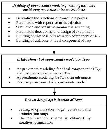
Figure 2.
The procedure of the proposed approach.
The simplified procedure for RDO of Tcpp considering manufacturing uncertainties with repetitive units is listed as follows:
- (a)
- The parametric FEA considering the uncertainties of the PMSM is conducted, and the most significant parameters are screened. DoE samples the parameters with and without tolerances. Through parametric FEA, the center values and manufacturing deviation rates of the parameters, as well as their corresponding ideal components and fluctuation components of Tcpp, are extracted, and the training database of the two components is established.
- (b)
- The approximate model of the ideal component and the fluctuation component of Tcpp are established, respectively. Then, the approximate model of Tcpp with tolerances is obtained by adding the two approximate models.
- (c)
- The optimization object function, constraint conditions, and parameter optimization range are defined, and the RDO model of Tcpp is established. The approximate model is embedded into the RDO model, and RDO obtains the optimization scheme that meets the mean and standard deviation requirements.
2.2. The Building of an Approximate Modeling Training Database Considering Repetitive Unit Uncertainties
The traditional PMSM FEA uses Ansys software to build a symmetrical or quarter-simplified model. The repetitive unit parameters in the same structure are treated equally, which cannot reflect the influence of the manufacturing uncertainties on the output characteristics. In order to consider the manufacturing processing dispersion of repetitive units, the repetitive units of the PMSM model should be assigned independently, so the parametric FEA method was adopted in this study to obtain the FEA model, which is consistent with the actual manufacturing conditions. On this basis, sensitivity analysis was carried out, and the significant design parameters were screened out. Then, the training database of approximate modeling was constructed according to the selected design parameters.
- (a)
- According to the relative position of each unit, the coordinate function containing the parameter value variable of repetitive units is established.
- (b)
- According to the actual values of input parameters, the coordinate functions are calculated to obtain the model with the actual values, and the Tcpp is extracted by simulation.
- (c)
- Single-factor sensitivity analysis selects the most significant factors affecting Tcpp. The formula for sensitivity analysis is shown as follows:
The parameters sensitive to Tcpp are screened out through sensitivity analysis, which is used as the design parameters for the following RDO research.
- (d)
- The training database was constructed.
A parametric FEA describing the actual motor parameters can be obtained based on the above analysis. Through the DoE, the sample data by the actual production dispersion of Tcpp are obtained by parametric FEA, which is used for approximate modeling training.
An approximate model was established in this study to fit the cogging torque of the PMSM as an example. Cogging torque can be considered a series of periodic waveforms. The peak-to-peak value of the cogging torque (Tcpp) is the difference between the maximum and minimum values of cogging torque in one or more cycles. In most existing studies, Tcpp is used to quantify cogging torque, which is defined as:
where Tcpp is the peak-to-peak value of cogging torque, Tcog is the cogging torque, and φ gives the rotor angle.
Tcpp = max (Tcog(φ)) − min (Tcog(φ)),
Assume a surface-mounted permanent magnet synchronous motor (PMSM) with P poles and Q slots, of which the schematic diagram of repetitive units of the PMSM is shown in Figure 3. Several uncertainties from a single source can be involved owing to repetitive units in the PMSM. Their variation of structures and material properties can be approximately regarded as random variables following a Gaussian distribution. In this paper, “repetitive units” is used to describe the structural characteristics of the PMSM.
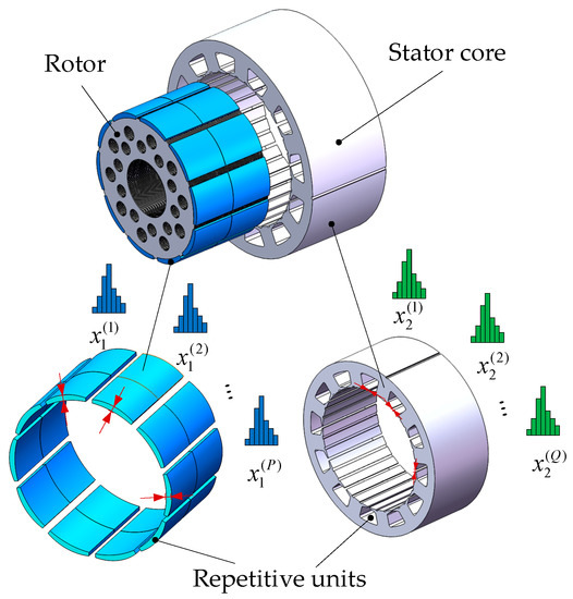
Figure 3.
Repetitive units of the permanent magnet synchronous motor (PMSM).
Consider a motor with K design parameters that has center value x = {x1, x2, …, xK}, where the deviations between actual design parameters and ideal center values can be presented as σ = {σ1, σ2, …, σK}, and the number of repetitive units of the kth design parameter is pk. Then, for convenience of expression, the center value after taking repetitive units into account can be expanded to X,
where = = … = . In manufacturing, the repetitive units of the PMSM inevitably have manufacturing deviations. Their corresponding deviations are expanded to Σ,
Thus, the design parameters of a motor make up a random variable Z,
which is assumed to form multivariate Gaussian distributions. The manufacturing deviation rate of each repetitive unit is defined as the ratio of the random parameter tolerance and its corresponding center value, which means the rate at the parameters changes. It can be represented as ζ,
Assume that f(Z) is the approximate function of the Tcpp, which can be presented as Equation (7) based on Taylor expansion:
If we omit the higher-order terms, Formula (7) can be expressed by first-order Taylor expansion as:
where X is the center values vector of design parameters, and Z is the design parameters vector with manufacturing deviations. Z − X is the deviation between the actual value and the center value of each parameter, that is, the manufacturing deviation of each design parameter. f′(X) is the gradient near the center value vector of the design parameter. Take the manufacturing deviation rate as ζ, that is, ζ =Σ/X = (Z − X)/X, then Equation (8) can be expressed as:
Equation (9) can be further transformed into:
that is,
If we use f1 to represent the first term in the bracket on the right, shown as ; and g1 to represent the second term in the bracket on the right, shown as .
Then, f(Z) can be expressed as:
In the process of approximate modeling, we first performed an approximate calculation of the first component to obtain . At this point, X is the input variable of the model, and as a known value, the gradient at this point is an unknown but constant value, which does not influence the approximate calculation of . Therefore, in the approximate calculation of the second component , only the input variable ζ, the manufacturing deviation rate, needs to be considered as the input variable. Equation (12) can be further written as:
Thus, the approximate model of Tcpp can be composed of two parts: the ideal component of Tcpp caused by the center value of the design parameters and the fluctuation component of Tcpp caused by the manufacturing deviation rate of the design parameters. On this basis, the approximate calculation of Tcpp can be performed on the ideal component and the fluctuation component in turn. Thus, the effects of center value X and manufacturing deviation rate ζ on Tcpp are decoupled to achieve the purpose of modeling separately.
In order to establish approximate modeling of the ideal component and the fluctuation component of Tcpp, the corresponding input data of the model are the center values and the manufacturing deviation rates of the design parameters. The procedure for establishing the corresponding training database is shown in Figure 4.
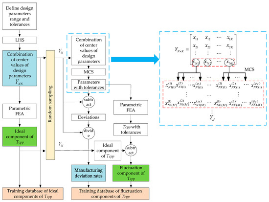
Figure 4.
The procedure of establishing the training database.
The steps to build the training database are as follows:
- (1)
- The design parameters range and tolerances are defined. For the filling of the design space, Latin hypercube sampling (LHS) [19] is used to sample combinations of center values of the design parameters in the design parameter range. Assuming that there are K design parameters, LHS obtains NN groups of center value combinations. Parametric FEA is performed on each group of samples to obtain Tcpp without tolerance, which, together with the sampling center values of design parameters, is the training database of ideal components of Tcpp constituted.
- (2)
- N samples are randomly selected from the NN groups of center values samples. Considering the manufacturing deviations of repetitive units, Monte Carlo sampling (MCS) for each group of design parameter center values can obtain the actual parameter values with manufacturing tolerances. As shown in the dashed box on the right of Figure 4, the numbers of their corresponding repetitive units for K design parameters can be presented by p1, p2, …, pK. According to experience, all design parameters are subject to the Gaussian distribution. Thus, MCS with Gaussian distribution performed M times for each group of center value combinations. The Nth group is taken as an example; the first design parameter xN1 contains p1 repetitive units, which can be expanded into , , …, , according to its manufacturing deviations in the first sampling. Other N-1 groups of parameters are sampled as this rule. In the end, a high-dimension matrix Yd is obtained, of which the dimension is d = N × M × pK. The Tcpp database with tolerances is obtained by parametric FEA, which subtracted the Tcpp ideal component with the center value of the corresponding design parameter to obtain the database of the Tcpp fluctuation component. In addition, the difference between the parameters with tolerances and the corresponding center values of design parameters is divided by the corresponding center values of design parameters to obtain the manufacturing deviation rate. The manufacturing deviation rate data, together with the fluctuation component of Tcpp, constitute the training database of fluctuation components of Tcpp.
2.3. The Establishment of the Approximate Model for Tcpp
According to the DoE of Section 2.2, we proposed the compensate fluctuation (CF) approximate modeling method, which established the approximate models for Tcpp considering manufacturing uncertainties of repetitive units. Based on the approximate modeling of the ideal component of Tcpp, the fluctuation component is supplemented and added to the ideal component model; that is, the ideal and fluctuation components of Tcpp are modeled and then added to obtain the Tcpp approximate model.
The proposed CF approximate modeling method is carried out for the two components. The flow chart of the proposed method is shown in Figure 5.
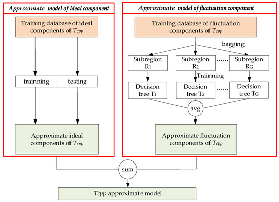
Figure 5.
The flow chart of the compensate fluctuation (CF) approximate modeling method.
Firstly, a conventional approximate modeling method is searched to establish the ideal component of Tcpp. The center values vector of design parameters X is the input data. f1(X) is the ideal component of Tcpp, the output data.
Secondly, for the fluctuation component of Tcpp, g1(ζ), that is g1((Z − X)/X), caused by manufacturing deviation rate (Z − X)/X, the random forest (RF) method [20] based on bagging [21,22] is used for the establishment of the approximate model. First, the subspaces of the fluctuation component training database are constructed. The manufacturing deviation rates and the corresponding Tcpp fluctuation component database obtained by DoE in Section 2.2 are sampled with replacement multiple times based on bagging, and various training database subspaces are obtained. The subspaces of the training database R1, R2, …, RG, and corresponding decision trees T1, T2, …, TG are obtained. Each subspace contained several pieces of training data from the entire training database, and the number of training data contained in all decision trees far exceeded the total number of the training database. Then, the database of each subspace Rg is trained to establish a decision tree Tg to approximate the fluctuation component of Tcpp. According to the information gained, the order of the input parameter features in the leaf nodes of the decision tree is determined. Then the training data are divided according to the judgment index of the input parameter features at each leaf node until it cannot be divided further. The training objective of each decision tree is to minimize the difference between the predicted fluctuation component from the output of the tree and the actual fluctuation component, which means that the tree’s output is close to the actual value. The training objective is shown as follows:
where yg is the actual fluctuation component of Tcpp, i.e., the FEA result; ζi is the ith manufacturing deviation rates vector from N × M samples and Tg(ζi) is the predicted value of Tcpp fluctuation component for the gth tree model.
When the model is used to approximate the fluctuation component of Tcpp, assuming that the number of the decision tree is G, the manufacturing deviation rates should be input to the fluctuation component model. Then the outputs of all decision trees are averaged to obtain the predicted value of the final fluctuation component of Tcpp as Equation (15):
where Tg(ζi) is the output of the gth decision tree; g1(ζ) is the predicted value of the fluctuation component of Tcpp.
Finally, the predicted Tcpp with tolerances can be calculated as the sum of the above two components, shown as:
The accuracy of the approximate model is evaluated by relative error (RE):
where ns is the number of selected test samples, and Yj(Xj, ζj) is the jth actual response value of the test sample, i.e., the parametric FEA value. (Xj, ζj,) is the jth predicted value of the approximate model. A poor RE reflects high model accuracy.
2.4. RDO of Tcpp Considering Repetitive Unit Parameter Uncertainties
Different combinations of design parameters affect the consistency of output characteristics of the PMSM. In order to improve the consistency of output characteristics of the batch PMSM, it is necessary to find some design schemes to make the mean values of the output characteristics as close as possible to the design object and distributed in a concentrated manner in the presence of manufacturing deviation while ensuring the performance also meets the requirements. In this study, the particle swarm optimization (PSO) method is used to optimize the design parameters and realize the robust design of the PMSM, considering the manufacturing uncertainties of repetitive units. The optimization objective function is shown in Equation (19). The optimization objective is to minimize the mean and standard deviation of the Tcpp of the PMSM, and the constraint is that the no-load back electromotive force (BEMF) is not lower than its threshold. The optimization will be stopped when the mean and standard deviation of the Tcpp are lower than their respective thresholds. The specific implementation is shown in Figure 6.
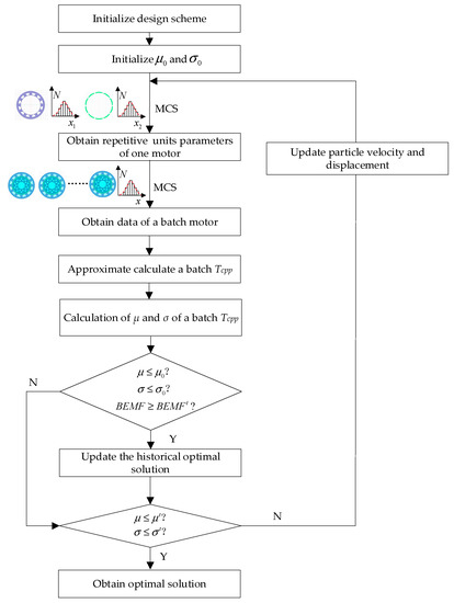
Figure 6.
Robust design optimization with repetitive unit uncertainties.
The steps of robust design optimization (RDO) with repetitive unit uncertainties are as follows:
Step 1, the design scheme: the mean value and standard deviation are initialized. The MCS is performed according to the actual manufacturing deviations to sample the parameters of the repetitive units in one motor. Then, MCS is performed according to the deviations of the batch motor to obtain the parameters of the batch motor. The approximate model is used to calculate the batch motor’s Tcpp value to calculate the batch motor’s statistical characteristics, such as the mean and standard deviation.
Step 2, the mean and standard deviation of the current scheme are compared with the historical scheme. If the current scheme is better than the historical scheme, it replaces the optimal one; Otherwise, the historical optimal solution is kept, and it is determined whether the optimization goal is achieved. If the optimization goal is achieved, the optimal solution is output. Otherwise, the particle position and velocity are updated, and steps 1 and 2 are repeated.
According to the optimal design scheme, MCS is carried out to obtain a batch of the motor according to the design tolerances, the parametric FEA is conducted, and the robustness of the optimized motor is verified. In addition, several prototypes are produced to test and verify the scheme’s effectiveness.
3. Case Study
3.1. Establishment of Parametric FEA and Screening of the Critical Design Parameters
A type of PMSM with 10p/12s was used to verify the proposed method, where the basic structure of the PMSM is shown in Figure 7. The speed of the permanent magnet synchronous motor (PMSM) parametric FEA model was set to 5 rpm. The fixed parameters that do not consider the tolerance are shown in Table 1. The variable parameters that consider tolerances are shown in Table 2.
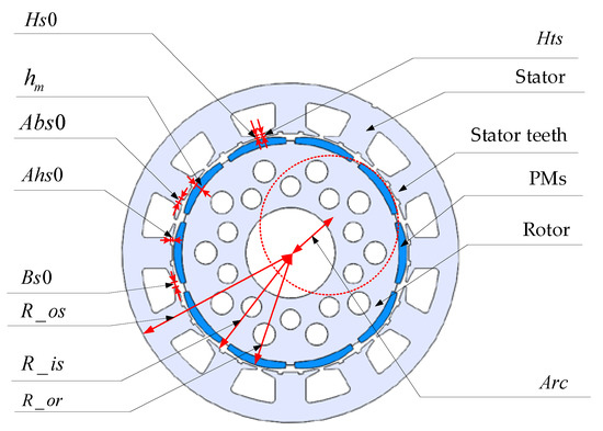
Figure 7.
The structure of the PMSM.

Table 1.
Fixed parameters of the permanent magnet synchronous motor (PMSM).
Table 2.
Variable parameters of the PMSM.
In traditional FEA, PMSM is regarded as an utterly symmetric model, and 1/4 of the ideal model is shown in Figure 8. The parameters of repetitive units were equal, regardless of the manufacturing deviations. The simulation Tcpp waveform was an ideal sine wave, which is shown in Figure 9. The ideal Tcpp was 0.089 Nm, and the measured Tcpp was 0.12 Nm. The RE with the FEA and the measured waveform was 26.8%. Therefore, it is necessary to carry out the FEA of the PMSM considering the manufacturing deviations of repetitive units, which can reflect the actual motor operation.
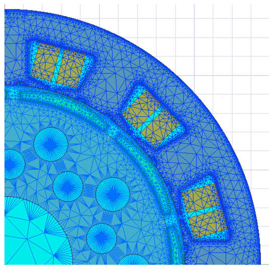
Figure 8.
The ideal model of the PMSM.
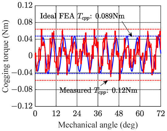
Figure 9.
Cogging torque waveform (measured and ideal FEA results).
In this study, parametric FEA was used to simulate the complete model of the PMSM. Firstly, the coordinate functions with design parameter variables were derived based on the position relationship between the repetitive units. Then, the coordinate function was input into the parameter form of the model. Then, according to Table 1, the fixed parameters were injected into the model. According to Table 2, MCS was conducted to sample variable parameters within the tolerance range. The parameters of the repetitive units were obtained and injected into the parametric FEA. The parametric FEA of the motor can simulate the operation situation considering repetitive units with tolerances, solving the problem that the traditional symmetry model treats repetitive units as the same value. The model part is shown in Figure 10.
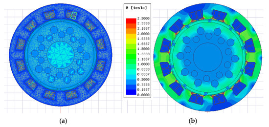
Figure 10.
Meshing and magnetic density analysis of the PMSM: (a) meshing; (b) magnetic density analysis.
The cogging torque waveform and BEMF waveform were calculated using the parametric FEA, and the results are shown in Figure 11. The Tcpp is 0.11 Nm for no-load operation, and the BEMF is 221.3 mV with parametric FEA. The test Tcpp is 0.12 Nm. The RE between the measured and FEA is about 8.3%, which verifies the accuracy of the simulation model. Therefore, the parametric FEA can be used in the following RDO research.

Figure 11.
The electrical characteristic of the PMSM: (a) cogging torque waveform (measured and parametric FEA results); (b) no-load back EMF.
Single factor sensitivity analysis was performed for the above eight variable parameters of the PMSM, and the remaining three fixed parameters were set at the center values as Table 1. The center value of each variable parameter was set to ±2.5% and ±5% of its initial design center value in turn, and MCS was conducted within the tolerances. Other factors remained unchanged, and the Tcpp with the change of a single factor was obtained.
The sensitivity analysis result is shown in Figure 12. The horizontal axis is shown as −0.05, −0.025, 0, 0.025, and 0.05, corresponding to the change levels (−5%, −2.5%, 0, 2.5%, 5%) for each parameter. It can be seen that the sensitivity of parameters is positively correlated to the variation range of Tcpp with the ±5% variation of parameters. The variation range of the parameters is shown in Table 3.
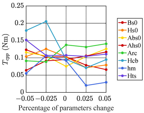
Figure 12.
Sensitivity analysis result.
Table 3.
The variation range of Tcpp.
The three parameters (Hcb, hm, and Bs0) with the most extensive Tcpp variation range of 0.1342, 0.0855, and 0.0547 Nm can be seen in Table 3. The three most sensitive parameters to cogging torque were screened out, including the width of stator slot opening Bs0, magnetic coercive force Hcb, and magnetic tile thickness hm.
3.2. Design of Experiment
The design parameters with tolerances were considered when conducting DoE. We first used LHS to obtain 120 groups of center values of the three design parameters. The output response, Tcpp of the model without tolerances, was simulated. The ideal components of Tcpp and center values of design parameters data were extracted to create the ideal component training database. Then, 30 group samples were randomly selected from the above 120 groups of center value samples. Fifty Monte Carlo sampling (MCS) groups were utilized for each sample, and 1500 samples with tolerances were obtained. The Tcpp values with tolerances were subtracted from the corresponding Tcpp values without tolerances to obtain the fluctuation component of Tcpp. By subtracting the center values of the parameters from the parameters with tolerances, the deviations of the design parameters were obtained, and then the corresponding manufacturing deviation rates were calculated. The manufacturing deviation rates of parameters and the fluctuation components of Tcpp constitute the database of fluctuation components.
3.3. Approximate Modeling and Error Analysis
For the 120 groups of samples obtained by DoE in Section 3.2, a conventional approximate method was sought to establish the ideal component of Tcpp. On this basis, the random forest based on bagging was used to conduct the approximate modeling of the fluctuation component of Tcpp. The bagging was used to sample the 1500 groups of fluctuation component data obtained in Section 3.2 with the replacement, 200 groups of data were sampled each time, and 50 decision trees were established. These decision trees cover the total sample space. When calculating the approximate fluctuation value of Tcpp, 50 decision trees gave predicted results according to their training. Then their average values were calculated to obtain approximate results of the fluctuation value of Tcpp. The approximate calculation process of the fluctuation component of Tcpp is shown in Figure 13.
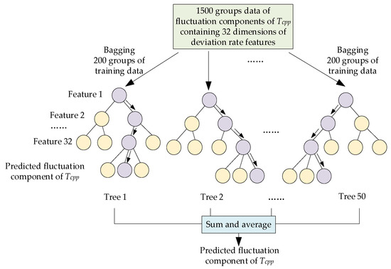
Figure 13.
The approximate calculation process of the fluctuation component of Tcpp.
In order to verify the accuracy of the approximate model, 80 different groups of testing samples with tolerances were sampled outside the training data. The approximate modeling process and the calculation results of the compensate fluctuation (CF) method proposed in this paper are shown in Figure 14. The Kriging modeling method was used to establish the ideal component of Tcpp, and the average RE between the approximate calculation and the parametric FEA is 11.7%, indicating that the ideal composition can be calculated with high accuracy by using the conventional approximate modeling method. The random forest method was adopted for the fluctuation components of Tcpp, and the average RE between the approximate calculation and the parametric FEA is 53.1%. This was due to the lower magnitude of the fluctuation component, making the RE value higher. However, the fluctuation component of Tcpp would be compensated for the ideal components, obtaining the approximate calculation of Tcpp considering tolerances, the average RE of which is 7.7%. This showed that the compensation of the ideal component model improves the overall approximate modeling accuracy.
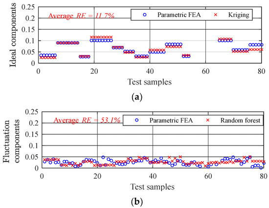
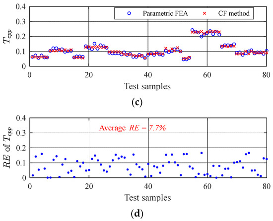
Figure 14.
The approximate process and results of the CF method proposed in this paper: (a) ideal components of Tcpp; (b) fluctuation components of Tcpp; (c) Tcpp with tolerances; (d) the average RE of the CF method.
In order to prove the effectiveness of the proposed approximate model, a single conventional approximate modeling method was used to approximate the high-dimensional input data and compare it with the CF method proposed in this paper. Firstly, the same amount of training data as the proposed CF method was used for conventional approximate modeling. The LHS was used to obtain 1500 groups of center values of design parameters. Each group was sampled according to the tolerances by MCS, and a set of samples with tolerances was obtained. They would be used as the training database of the Kriging model or random forest model. Then, the above 80 groups of test samples were used for verification. The high-dimensional approximation using the Kriging or random forest method compared with the CF method proposed in this paper is shown in Figure 15.
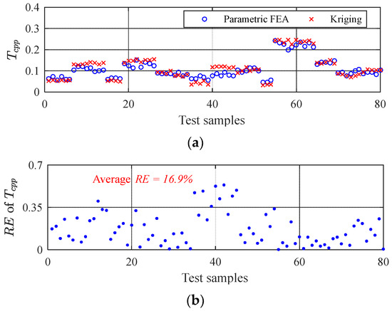
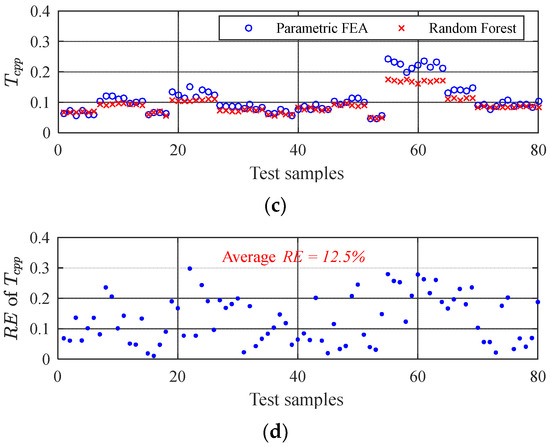
Figure 15.
Single conventional approximate modeling: (a) Kriging approximate modeling; (b) the RE of Kriging; (c) random forest approximate modeling; (d) the average RE of random forest.
The average RE of the approximate modeling method is listed in Table 4. It can be seen that the average RE values of high-dimensional input using the Kriging or random forest model are 16.9% and 12.5%. The average RE of the CF method proposed in this paper was 7.7%, 54.4%, and 38.4% lower than the above two conventional methods. The effectiveness of the proposed CF approximate modeling method was verified. The CF approximate model has high accuracy, meeting the requirement of RDO for Tcpp.
Table 4.
The combination of RE of the CF method and conventional method.
3.4. Robust Design Optimization of Tcpp
Based on the proposed method, we carried out RDO based on the PSO algorithm. The optimization objective is to minimize the mean value and standard deviation of Tcpp. The original BEMF of the mass production motor is 221 mV; a motor with a BEMF drop of less than 10% after optimization would ensure that the heat of the optimized motor is within the allowable range. The BEMF should be constrained to no less than 190 mV. The convergence condition of the optimization is that the mean value of Tcpp is not more than 0.1 Nm, and the standard deviation of Tcpp is not more than 0.02 Nm. The optimization objective function is shown as follows:
The proposed approximate model was embedded into the PSO algorithm for RDO. The initial particle number was set to 10; the population size was set to 100. The optimization results of mean values and standard deviation of Tcpp are shown in Figure 16.
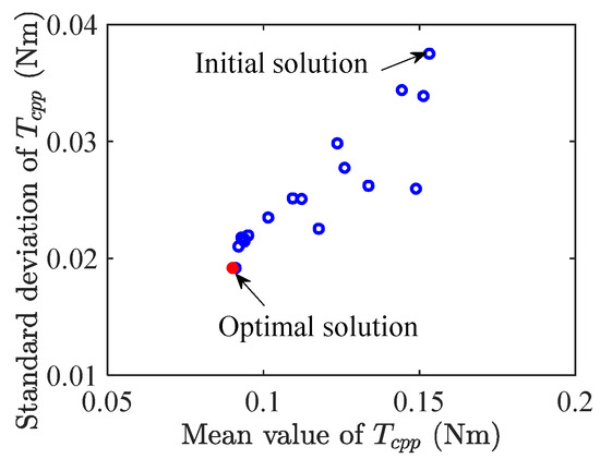
Figure 16.
The optimization results.
After 150 iterations, the optimized scheme was obtained. The center values of hm, Bs0, and Hcb were designed to be 2.6 mm, 2 mm, and −1,038,100 A/m. The optimization results and the initial design scheme are shown in Table 5.
Table 5.
Initial and robust optimal design of the PMSM.
In order to preliminarily verify the effectiveness of the optimization scheme with the uncertainties range, 10,000 groups of design parameters with tolerances on initial and RDO schemes were sampled through MCS, and their Tcpp values were calculated with the CF approximate model. Figure 17 shows the MCS results of the initial and RDO models. The robustness and electromagnetic performance of the initial and RDO schemes are shown in Table 6. Compared to the initial scheme, the mean value of the Tcpp is reduced by about 42.3% in the RDO model, which is close to the ideal situation without tolerances. The standard deviation is reduced by 48.6%, which shows that the optimized motor is less affected by noise factors, and the batch cogging torque is more stable than the initial. BEMF is slightly decreased by 8.2% and is within the acceptable range.
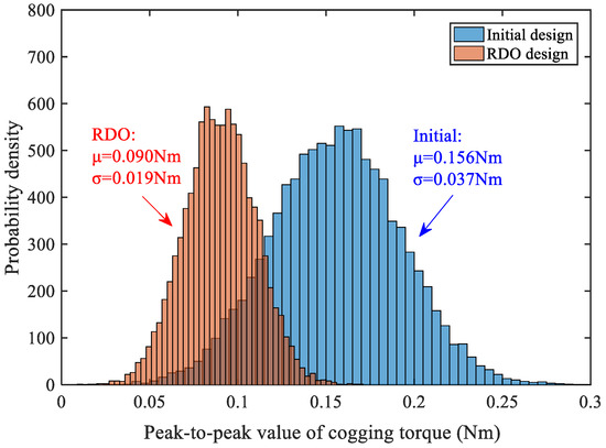
Figure 17.
Cogging torque distribution based on Monte Carlo simulation.
Table 6.
Robustness and performance comparison of the PMSM before and after optimization.
In order to further verify the practical effect of RDO on the PMSM, 18 prototypes of the RDO scheme and initial scheme were mass-produced, and experiments were carried out. The test setup for the cogging torque of the prototypes is shown in Figure 18. It consists of four parts: test bench, power supply, server, and data acquisition upper computer. The test bench includes the prime motor, speed reducer, torque sensor, coupling, and the prototype to be tested. The prime motor is decelerated by a 64:1 speed reducer connected to the motor’s coupling to be tested. The speed of the motor to be tested is kept at 5 rpm.
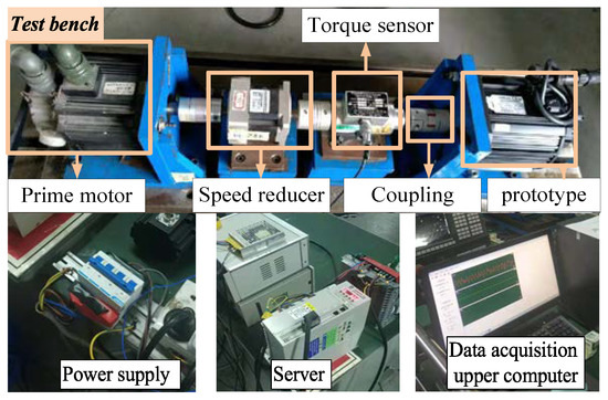
Figure 18.
Test setup for the cogging torque of the prototypes.
Figure 19 shows the Tcpp distribution of initial and RDO schemes in the prototypes. It can be seen that the mean value of Tcpp decreases from 0.146 to 0.104 Nm, a reduction of 28.8%, while the standard deviation decreases from 0.032 to 0.016 Nm, a 50% reduction. The actual decrease degree of the optimized mean value of the cogging torque in the prototype is lower than that of MCS. This may be because some parameters in the manufacturing process were not fully controlled within the optimization target. The assembly process had errors due to inevitable human factors, resulting in the optimization degree of the actual prototype batch being lower than the simulation.
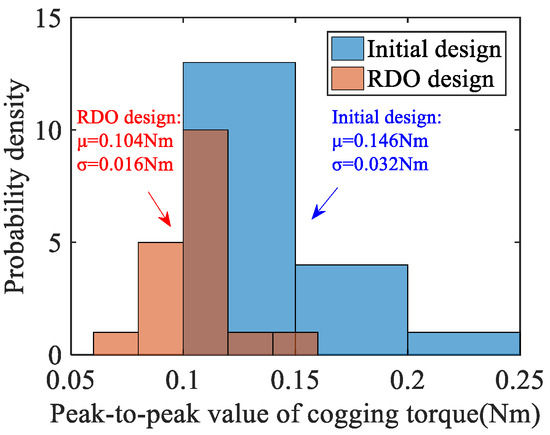
Figure 19.
Tcpp distribution of initial and RDO schemes in prototypes.
4. Conclusions
There remain significant challenges in considering the inevitable repetitive unit uncertainties and considering the calculation efficiency due to uncertainties from manufacturing dispersion. Aiming at these challenges, a compensate fluctuation (CF) approximate modeling method is proposed in this paper as a surrogate for the finite element analysis. It was applied to the robust design optimization (RDO) process of the Permanent magnet synchronous motors (PMSM). In this method, based on the ideal component model, the fluctuation component model is supplemented and compensates for the ideal model to obtain the approximate model by considering the uncertainties of the repetitive units. It solves the approximate modeling problem of considering the uncertainties of multiple-parameter repetitive units in the RDO. Applying this CF model to RDO gave a design scheme with a minimal fluctuation effect. Based on the results, the following conclusions are drawn:
- (1)
- The CF approximate model proposed here can significantly improve the calculation efficiency and accuracy of the critical output response of the PMSM, effectively solving the computing issue and the quality evaluation and optimization of the PMSM. This can apply to problems considering and not considering the repetitive unit uncertainties. The RDO method based on the proposed CF approximate model can consider multiple design parameters and does not distinguish the source of the uncertainties; thus, robustness with various uncertainties can be guaranteed.
- (2)
- Based on the ideal model, the CF approximate modeling method compensates for the fluctuation component caused by manufacturing uncertainties. For the ideal component of the Tcpp, the conventional approximation modeling method was used to obtain accurate approximate calculation results with fewer training data. On this basis, the fluctuation component model compensates for the fluctuation caused by uncertainties. Compared with the conventional single approximation model, it is proved that the CF model has higher accuracy. It provides a new idea for approximate modeling considering the manufacturing deviations of multiple-parameter repetitive units. The analysis of the case study showed that the average RE of the approximate model is about 7.7%, which is 54.4% and 38.4% lower than those using single conventional Kriging or random forest methods.
- (3)
- To realize the RDO of the PMSM with the manufacturing dispersion of multiple parameters, an RDO model based on CF approximate modeling was proposed. The RDO model proposed in this paper can comprehensively consider the effect of multiple-parameter repetitive-unit manufacturing deviations and can provide a new direction for the RDO of multiple parameters. The results of the PMSM robustness in the case study showed a significant improvement. According to the Monte Carlo sampling (MCS) simulation, the mean value of the Tcpp decreased from 0.156 to 0.09 Nm (decreased by 42.3%), and the standard deviation decreased from 0.037 to 0.019 Nm (decreased by 48.6%). In prototype tests, the mean value and standard deviation of the Tcpp after the RDO decreased by 28.8% and 50%, respectively. It is possible to analyze the mean drop of the prototype, which results from some parameters in the actual production and assembly process not being wholly controlled within the optimization objective and inevitable human factors causing some errors. These reasons lead to a decrease in the mean value of the actual cogging torque, while the decrease degree is lower than that of the MCS. Future research will consider these random errors in the FEA model and RDO process.
Author Contributions
Conceptualization, L.W. (Liqin Wu); methodology, L.W. (Liqin Wu) and T.Y.; software, L.W. (Liqin Wu), C.S. and L.W. (Lin Wang); validation, L.W. (Liqin Wu), H.C., T.Y., C.S. and L.W. (Lin Wang); formal analysis, L.W. (Liqin Wu); investigation, L.W. (Liqin Wu) and T.Y.; resources, H.C.; data curation, L.W. (Liqin Wu), H.C., T.Y., C.S. and L.W. (Lin Wang); writing—original draft preparation, L.W. (Liqin Wu); writing—review and editing, X.Y. and G.Z.; visualization, X.Y. and G.Z.; supervision, X.Y. and G.Z.; project administration, X.Y. and G.Z.; funding acquisition, X.Y. and G.Z. All authors have read and agreed to the published version of the manuscript.
Funding
This research was funded by National Natural Science Foundation of China [grant number 52177134].
Data Availability Statement
Not applicable.
Conflicts of Interest
The authors declare no conflict of interest.
Nomenclature
| PMSM | Permanent magnet synchronous motor |
| RDO | Robust design optimization |
| FEA | Finite element analysis |
| Tcpp | The peak-to-peak value of cogging torque |
| DoE | Design of experiments |
| SVM | Support vector machine |
| RF | Random forest |
| Si | Sensitivity of the parameter to the target |
| xi | The value of the ith parameter |
| x0 | The center value of the ith parameter |
| Δxi | Incremental of the parameter |
| MCS | Monte Carlo sampling |
| Tcog | The cogging torque |
| φ | The rotor angle |
| P | The number of poles |
| Q | The number of slots |
| K | The number of design parameters |
| x = {x1, x2, …, xK} | The center value vector of design parameters |
| σ = {σ1, σ2, …, σK} | The deviations between actual design parameters and ideal center values |
| k | One of the design parameters |
| pk | The number of repetitive units of the kth design parameter |
| X | The center value vector taking repetitive units into account |
| The center value of the pkth repetitive unit of the kth design parameter | |
| Σ | The deviations between actual design parameters and ideal center values taking repetitive units into account |
| The deviations of the pkth repetitive unit of the kth design parameter | |
| Z | The random variable of design parameters |
| The variable of the pkth repetitive unit of the kth design parameter | |
| ζ | The manufacturing deviation rate |
| / | The manufacturing deviation rate of the pkth repetitive unit of the kth design parameter |
| LHS | Latin hypercube sampling |
| NN | The number of groups of center value combinations in LHS |
| N | The number of groups of samples randomly selected from the NN groups of center values samples |
| The first design parameter xN1 containing p1 repetitive units of the Nth sample | |
| Yd | The matrix of the training data samples |
| M | The number of samples of Monte Carlo sampling of each group of center value combination |
| d | The dimension of the training data samples |
| CF | Compensate fluctuation |
| G | The number of subspaces or the decision trees |
| RG | The Gth subspace of the training database |
| TG | The Gth decision tree |
| g | One of the subspaces |
| yg | The actual fluctuation component of Tcpp, i.e., the FEA result |
| Tg | The predicted value of Tcpp fluctuation component for the gth tree model |
| The predicted peak-to-peak value of cogging torque | |
| RE | Relative error |
| ns | The number of selected test samples |
| Yj | The actual response value of the test sample |
| The predicted value of the approximate model | |
| PSO | Particle swarm optimization |
| F | The optimization object |
| BEMF | The no-load back electromotive force |
| BEMFt | Threshold value of the no-load back electromotive force |
| The mean value | |
| The standard deviation | |
| The initial mean value | |
| The initial standard deviation | |
| The optimization object value of the mean value | |
| The optimization object value of the standard deviation | |
| R_os | Outer radius of stator |
| R_is | Inner radius of stator |
| R_or | Outer radius of rotor |
| Bs0 | Width of stator slot opening |
| Hs0 | Depth of stator slot opening |
| Abs0 | Width of additional stator slot opening |
| Ahs0 | Depth of additional stator slot opening |
| Arc | Magnetic tile pole arc eccentricity |
| Hcb | Magnetic coercive force |
| hm | Magnetic tile thickness |
| Hts | Height of stator teeth |
References
- Chu, L.; Jia, Y.; Chen, D.; Xu, N.; Wang, Y.; Tang, X.; Xu, Z. Research on control strategies of an open-end winding permanent magnet synchronous driving motor (OW-PMSM)-equipped dual inverter with a switchable winding mode for electric vehicles. Energies 2017, 10, 616. [Google Scholar] [CrossRef]
- Nasr, A.; Gu, C.; Bozhko, S.; Bozhko, S.; Gerada, C. Performance enhancement of direct torque-controlled permanent magnet synchronous motor with a flexible switching table. Energies 2020, 13, 1907. [Google Scholar] [CrossRef]
- Zheng, P.; Wu, F.; Sui, Y.; Wang, P.; Lei, Y.; Wang, H. Harmonic analysis and fault-tolerant capability of a semi-12-phase permanent-magnet synchronous machine used for EVs. Energies 2012, 5, 3586–3607. [Google Scholar] [CrossRef]
- Ullah, K.; Guzinski, J.; Mirza, A.F. Critical review on robust speed control techniques for permanent magnet synchronous motor (PMSM) speed regulation. Energies 2022, 15, 1235. [Google Scholar] [CrossRef]
- Mohd, Z.F.; Mekhilef, S.; Mubin, M. Robust Speed Control of PMSM Using Sliding Mode Control (SMC)—A Review. Energies 2019, 12, 1669. [Google Scholar] [CrossRef]
- Jang, J.; Cho, S.; Lee, S.J.; Kim, K.; Kim, J.; Hong, J.; Lee, T. Reliability-based robust design optimization with kernel density estimation for electric power steering motor considering manufacturing uncertainties. IEEE Trans. Magn. 2015, 51, 1–4. [Google Scholar] [CrossRef]
- Lei, G.; Zhu, J.; Guo, Y.; Liu, C.; Ma, B. A review of design optimization methods for electrical machines. Energies 2017, 10, 1962. [Google Scholar] [CrossRef]
- Tanmoy, C.; Souvik, C.; Rajib, C. A Critical Review of Surrogate Assisted Robust Design Optimization. Arch. Comput. Methods Eng. 2019, 26, 245–274. [Google Scholar]
- Ji-Min, K.; Myung-Hwan, Y.; Jung-Pyo, H.; Sung-Il, K. Analysis of cogging torque caused by manufacturing tolerances of surface-mounted permanent magnet synchronous motor for electric power steering. IET Electr. Power Appl. 2016, 10, 691–696. [Google Scholar]
- Cressie, N. The origins of kriging. Math. Geol. 1990, 22, 239–252. [Google Scholar] [CrossRef]
- Ibrahim, I.; Silva, R.; Mohammadi, M.; Ghorbanian, V.; Lowther, D.A. Surrogate-based acoustic noise prediction of electric Motors. IEEE Trans. Magn. 2020, 56, 1–4. [Google Scholar] [CrossRef]
- Karaoglan, A.D.; Ocaktan, D.G.; Oral, A.; Perin, D. Design optimization of magnetic flux distribution for PMG by using response surface methodology. IEEE Trans. Magn. 2020, 56, 1–9. [Google Scholar] [CrossRef]
- Kim, S.; Lee, S.G.; Kim, J.M.; Lee, T.H.; Lim, M.S. Robust design optimization of surface-mounted permanent magnet synchronous motor using uncertainty characterization by bootstrap method. IEEE Trans. Energy Convers. 2020, 35, 2056–2065. [Google Scholar] [CrossRef]
- Lee, D.; Jeong, C.; Hur, J. Analysis of cogging torque and torque ripple according to unevenly magnetized permanent magnets pattern in PMSM. 2017 IEEE Transactions on Energy Conversion. In Proceedings of the 2017 IEEE Energy Conversion Congress and Exposition (ECCE), Cincinnati, OH, USA, 1–5 October 2017; pp. 2433–2438. [Google Scholar]
- Lee, S.G.; Kim, S.; Park, J.C.; Park, M.R.; Lee, T.H. Robust Design Optimization of SPMSM for Robotic Actuator Considering Assembly Imperfection of Segmented Stator Core. IEEE Trans. Energy Convers. 2020, 35, 2076–2085. [Google Scholar] [CrossRef]
- Ou, J.; Liu, Y.; Qu, R.; Doppelbauer, M. Experimental and theoretical research on cogging torque of PM synchronous motors considering manufacturing tolerances. IEEE Trans. Ind. Electron. 2017, 65, 3772–3783. [Google Scholar] [CrossRef]
- Yang, Y.; Bianchi, N.; Bramerdorfer, G.; Zhang, C.; Zhang, S. Methods to improve the cogging torque robustness under manufacturing tolerances for the permanent magnet synchronous machine. IEEE Trans. Energy Convers. 2020, 36, 2152–2162. [Google Scholar] [CrossRef]
- Yang, Y.; Bianchi, N.; Zhang, C.; Zhu, X.; Liu, H.; Zhang, S. A method for evaluating the Worst-Case cogging torque under manufacturing uncertainties. IEEE Trans. Energy Convers. 2020, 35, 1837–1848. [Google Scholar] [CrossRef]
- Ma, Y.; Xiao, Y.; Wang, J.; Zhou, L. Multicriteria optimal Latin Hypercube design-based surrogate-assisted design optimization for a permanent-magnet vernier machine. IEEE Trans. Magn. 2021, 58, 1–5. [Google Scholar] [CrossRef]
- Svetnik, V.; Liaw, A.; Tong, C.; Culberson, J.C.; Sheridan, R.P.; Feuston, B.P. Random Forest: A Classification and Regression Tool for Compound Classification and QSAR Modeling. J. Chem. Inf. Model. 2003, 43, 1947–1958. [Google Scholar] [CrossRef] [PubMed]
- Breiman, L. Bagging predictors. Mach. Learn. 1996, 24, 123–140. [Google Scholar] [CrossRef]
- Bühlmann, P.; Yu, B. Analyzing bagging. Ann. Stat. 2002, 30, 927–961. [Google Scholar] [CrossRef]


Disclaimer/Publisher’s Note: The statements, opinions and data contained in all publications are solely those of the individual author(s) and contributor(s) and not of MDPI and/or the editor(s). MDPI and/or the editor(s) disclaim responsibility for any injury to people or property resulting from any ideas, methods, instructions or products referred to in the content. |
© 2023 by the authors. Licensee MDPI, Basel, Switzerland. This article is an open access article distributed under the terms and conditions of the Creative Commons Attribution (CC BY) license (https://creativecommons.org/licenses/by/4.0/).