Article

Predicting the Performance of PEM Fuel Cells by Determining Dehydration or Flooding in the Cell Using Machine Learning Models

1
Dhanushkodi Research Group, Department of Chemical Engineering, Vellore Institute of Technology, Vellore 632014, India
2
Automotive Research Centre, Vellore Institute of Technology, Vellore 632014, India
3
Department of Energy, Cracow University of Technology, 31-864 Cracow, Poland
4
Institute of Thermal Power Engineering, Cracow University of Technology, 31-864 Cracow, Poland
*
Authors to whom correspondence should be addressed.
Energies 2023, 16(19), 6968; https://doi.org/10.3390/en16196968
Submission received: 17 August 2023 / Revised: 10 September 2023 / Accepted: 15 September 2023 / Published: 6 October 2023
(This article belongs to the Special Issue Advanced Research on Fuel Cells and Hydrogen Energy Conversion)

Abstract

:
Modern industries encourages the use of hydrogen as an energy carrier to decarbonize the electricity grid, Polymeric Electrolyte membrane fuel cell which uses hydrogen as a fuel to produce electricity, is an efficient and reliable ‘power to gas’ technology. However, a key issue obstructing the advancement of PEMFCs is the unpredictability of their performance and failure events caused by flooding and dehydration. The accurate prediction of these two events is required to avoid any catastrophic failure in the cell. A typical approach used to predict failure modes relies on modeling failure-induced performance losses and monitoring the voltage of a cell. Data-driven machine learning models must be developed to address these challenges. Herein, we present a machine learning model for the prediction of the failure modes of operating cells. The model predicted the relative humidity of a cell by considering the cell voltage and current density as the input parameters. Advanced regression techniques, such as support vector machine, decision tree regression, random forest regression and artificial neural network, were used to improve the predictions. Features related to the model were derived from cell polarization data. The model’s results were validated with real-time test data obtained from the cell. The statistical machine learning models accurately provided information on the flooding- and dehydration-induced failure events.

1. Introduction

Combustion engines used in cars and trucks constitute up to approximately 17% of carbon dioxide emissions and contribute to the increase in greenhouse gases in the atmosphere. Therefore, radical decarbonization is required to phase out fossil fuels. Scaling up renewable energy and accelerating the goals of clean energy initiatives can reduce greenhouse gases emissions by 50% by 2050. Issues related to power quality and instability affect the induction of renewable energy sources, such as solar, into electricity grids. The challenges that need to be overcome to expedite a stable, renewable energy storage system have still not been addressed by the energy industry. Therefore, the global energy market is transitioning towards sustainable, green, and clean hydrogen energy chiefly due to the growing distress related to climatic-change-related issues. The use of polymer electrolyte membrane fuel cells (PEMFCs) is one such approach that can be adopted to reduce carbon emissions and greenhouse gases. They convert chemical energy into electricity with a 60% efficiency. They use green hydrogen as fuel, which acts as a stable and efficient power source for gas energy storage systems in modern gas–electricity grids and transportation sectors.
A PEMFC is a two-electrode electrochemical cell that comprises a cathode, anode, gas diffusion layer (GDL), and an electrolyte barrier. Hydrogen is supplied to the anode side, while air is supplied to the cathode side. In this cell, electrons travel from the anode to the cathode via an external circuit, while protons travel through the selective polymer electrolyte membrane to the cathode. Water is the main by-product formed in the cell, which is due to oxygen reduction reactions at the electrode’s surface. No harmful discharge is emitted from its cell components during this process. The gas diffusion layer is a key component of PEMFCs, and it ensures the uniform distribution of reactive gases and the ejection of water molecules from the cell. A highly durable GDL material increases the lifespan of PEMFCs and facilitates the transport of electrons to and from the external circuit [1]. However, the build-up of too much water at the interfaces of the GDL–bipolar channels of the cell clogs the pores of the GDL and hinders the transport of oxygen into the catalyst layer (CL). This phenomenon is called ‘flow channel flooding’. This occurs when the cell operates at high current densities (>1.7 Acm−2), reducing the rate of ORRs and the performance of the cell. When flooding, the performance of the cell is reduced when reactants are not adequately hydrated with water molecules. Subsequently, the lack of water molecules in the reactants stream across the interfaces of the cell components is termed ‘dehydration’, which affects the durability of the membrane electrode assembly in the cell. In a dehydration-induced failure mode, the contact resistance of the membrane increases and the ionic conductivity decreases [2]. Therefore, the interface of the membrane–GDL must hold the optimum level of water to provide reliable cell performance. Thus, the selection of the GDL for the cell plays an important role in distributing the humidified reactant gases to the catalyst layer and removing excess water from the electrode’s surface to the bipolar plate channels. Poor selection of the GDL or its microporous layer material can lead to either severe flooding- or dehydration-induced failure modes in operating cells.
The conventional diagnostic tools used to visualize the transportation of water in the cell are neutron radiography, magnetic resonance imaging, X-ray microtomography, and direct optical visualization. These tools are expensive and require a differently designed fuel cell than those conventionally used. Thus, there is the need to develop universal noninvasive diagnostic tools that are economical and can work on all types of cells. The predictability of the failure modes using mathematical modeling is essential to increase the lifespan of the cell. Modeling of the dehydration or flooding phenomena involves mainly two different approaches: finite volume and data-driven empirical modeling. Springer et al. [3] and Bernardi and Verbrugge [4] modeled the steady-state and isothermal behavior of a PEM cell. For the finite volume modeling, a two-phase flow was considered. They predicted the performance of the cell at different levels of humidification. A two-phase flow model is derived based on the assumption that the liquid water forms inside the flow channel, while the reactant gas species enter via the catalyst’s surface [5]. The performance of a fuel cell modeled using CFD is primarily characterized with a polarization curve, which is calculated using Butler–Volmer reaction kinetics [6]. This requires parameters such as the open circuit voltage and the exchange current density to compute the performance of the cell. The parameters are calculated either experimentally or by evaluating zero-dimension equations [6]. Thus, for the convergence of the finite volume model, a multitude of assumptions are made, which might not provide accurate results all the time. Although extensive multiscale finite volume modeling is performed to assess the flooding- and dehydration-induced failures of PEMFCs, identifying a simple data-driven model that has high predictive accuracy is an emerging challenge for the fuel cell system. Accurate algorithms and statistical models are needed to diagnose the failure pathways, durability, and performance of the GDL materials. Furthermore, understanding the failure modes of the GDL is complicated when the cell operates at a high current density in the load mode. High current operating conditions can accelerate flooding in the channels, which can lead to both the catalyst’s and GDL’s corrosion, making it exceptionally difficult to isolate the failure modes of the GDL from the catalyst layer.
Machine learning algorithms and data-driven models are useful in assessing and isolating the failure modes of the GDL [6,7]. Openly available datasets related to failure modes using standardized operating data from fuel cell systems are essential to construct ML-based diagnostic models, which generally use algebraic and differential equations to simulate the cell degradation processes. ML-based data-driven models can be interpretable and used to rapidly assess the failure pattern of a GDL using relative humidity as a metric. In addition, ML-based models can generate hundreds of equations to simplify the localized failure points across the GDL–bipolar plate and GDL-CL interfaces in the fuel cell. They adopt empirical approaches and statistical modeling that have been proven as assumption free and able to capture the voltage–current–time trends using training datasets obtained from operating cells. This approach could be used to model any extreme conditions, such as dehydration and flooding. ML models have the ability to determine whether the composition and assembly of the GDLs are optimal for the given performance of the cell.
Thus, there is a need to develop universal noninvasive machine-learning-based diagnostic tools that are economical and work on all types of fuel cells. With this motivation, we developed a standardized workflow for a diagnostic tool consisting of three processing modules, which can be used to predict the performance of a fuel cell under conditions of flooding or dehydration. The first step involves data acquisition, followed by feature selection and, finally, regression model building. In this study, we used supervised machine learning techniques, namely, support vector machine regression (SVR), decision tree regression (DT), random forest regression (RF) and artificial neural network (ANN), to predict the output voltage of a PEM cell. Table 1 summarizes the machine learning models used to predict the parameters that could affect the GDL. Based on extensively collected data in the literature, our paper includes a data-driven machine learning method to predict the performance of a PEM cell by predicting the relative humidity using the cell voltage and current density. The objective of this study was to (a) analyze the importance of relative humidity in dehydration and flooding prediction; (b) compare and contrast four different machine-learning-based data-driven models that were used to assess the performance of the PEM cell by predicting the relative humidity; and (c) showcase how these models can address the problem of flooding and dehydration.

2. Materials and Methods

2.1. Data Acquisition

The data for the training and testing set were obtained from various polarization curves in research carried out by Dhanushkodi et al., Zhang et al. and Saleh et al. [11,12,13]. Several factors affect the relationship between the current density and the terminal voltage of a fuel cell, including temperature, air pressure, relative humidity, air flow rate, hydrogen pressure and membrane humidity of which relative humidity was chosen, while the rest were kept constant [14]. Relative humidity is one of the most important parameters in determining a cell’s voltage, as it can be directly related to the dehydration or flooding capacity of the cell, and it is relatively easy to measure [15]. A higher relative humidity indicates more water build-up in the cell (i.e., flooding), while a lower level of humidity indicates a lack of water in the cell (more contact resistance). In the case of limited GDL flooding in a cell, the voltage increases.
RH = f(i, V)
where V is the terminal voltage, i is the current density and RH is the relative humidity of the cell. There was an 80:20 split performed on the data, whereby 80% of the data were used as a training set, and the remaining 20% of the data were used as a testing set (Table 2).

Data Preprocessing and Scaling

The data were scaled using a standard scaling function, which finds the mean of the features and scales to unit variance.

2.2. Feature Selection/Importance

Given that not all of the features available in a dataset are equally essential, feature selection is a technique used to find insignificant features in a dataset, as not all features have an impact on the results. In this way, we aimed to decrease the size of the data before feeding it to the training model. Consequently, feature selection was carried out prior to training the machine learning models. The ability of models to explain is better using fewer features, and it is simpler to develop machine learning models with fewer features. This is mainly conducted to improve the efficiency of the ML, reduce the training time and avoid overfitting by reducing the redundancies. Similar to Ding et al., a feature selection can be performed in the case of a larger number of input features. An example of feature selection was performed on our dataset.
We used an extra trees classifier (Figure 1a) for the feature selection, which is also a type of ensemble learning that fits many randomized decision trees to various subsamples of the dataset. The initial training sample was used to build each decision tree in the extra trees forest. Then, each tree was given a random sample of k features from the feature set at each test node, and it must choose the best feature to divide the data according to certain mathematical criteria (typically the Gini Index). There were numerous de-correlated decision trees produced as a result of this random sampling of features. A score, which is calculated for all of the input features, represents the importance of each feature. A higher score implies that the particular feature will have a greater effect on the model. In Figure 1a, we can observe that the current density received the highest score of 0.56, while the voltage received a score of 0.44.

2.3. Machine Learning Models

This section describes the theory underlying the various soft computing models used. The overall modeling approach is presented as a block diagram in Figure 1b.

2.3.1. Support Vector Regression

This supervised learning method uses a decision boundary called the hyperplane (the best fit line) to fit the maximum number of points on it. Unlike other regression algorithms that work on a principle of minimizing the error between the predicted and actual values, this algorithm fits the hyperplane within the threshold value. The equation for this is an algorithm given by
L S V R = min e ( 1 2 W T W ) + C e T e
where W is the weight of the slope; C is the hyperparameter, the value of which was taken as 14 after hyperparameter tuning; and e is the intercept. To transform the data into a higher dimension (n-dimensional feature space), we used a radial-based kernel: soft margin kernel. SVR needs much fewer computations and produces results with higher accuracy. We can see that, in our study, it outperformed the other models and had the highest accuracy [16,17].

2.3.2. Decision Tree Regression

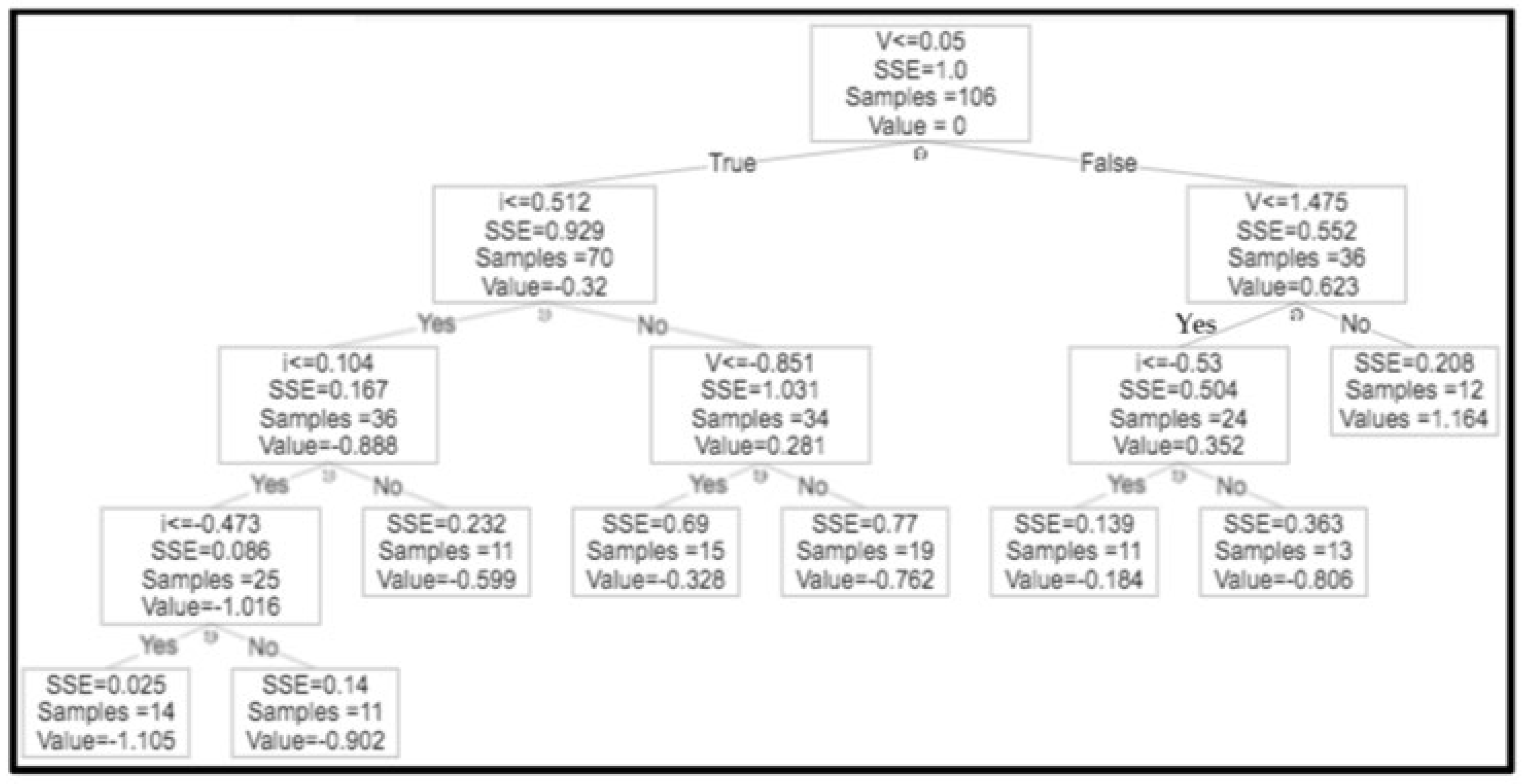
This tree-based supervised machine learning algorithm predicts the numeric outcome of the dependent variable by identifying the local region in a sequence of recursive splits in a smaller number of steps. There are three types of nodes: initial node, known as the root node; interior nodes; and leaf nodes. The root node, which is selected by minimizing the entropy, represents the complete sample, and it may be divided into other nodes. The branches represent the decision criteria, while the interior nodes reflect the characteristics of the data collection. The result is represented by the leaf nodes at the end. Each node applies a test to an input, and according to the results, one of the branches is chosen. Starting from the root, this process is repeated recursively until reaching a leaf node, at which time the value that entered the leaf serves as the output. The decision tree for our model is shown in Figure 2. The greatest advantage of this method is that its performance is not affected by nonlinearity. For our model, the maximum depth of the tree was taken as 5, and the minimum number of samples at the leaf node was taken as 2. Minimum hyperparameter tunning was required for this method [18,19].

2.3.3. Random Forest Regression

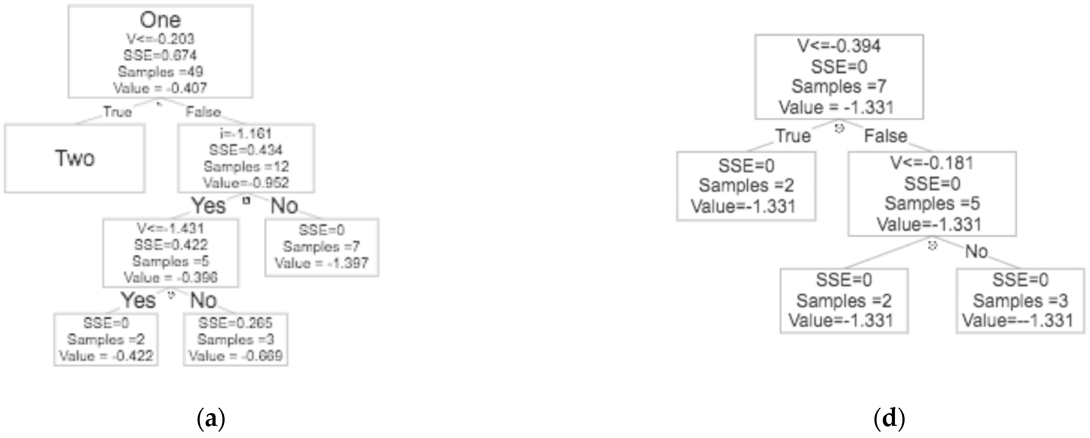
This type of supervised learning algorithm is based on the ensemble learning of a collection of decision trees. The subsets of the original data are created during training, which is known as bagging. Thus, many nonintersecting trees are created during training, the results of many decision trees are aggregated, and the optimal results are displayed as the final predicted value. This model efficiently works with less feature space, which is evident in our results. The last decision tree in our random forest is shown in Figure 3. In our model, 350 trees were used, with 2 as the minimum number of samples required at the leaf nodes. These parameters were obtained upon hyperparameter tuning. We can observe that the random forest model outperformed the decision tree model [20,21].

2.3.4. Artificial Neural Network

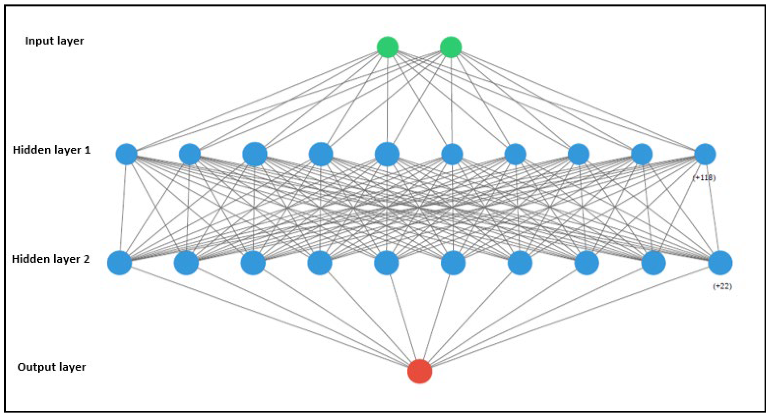
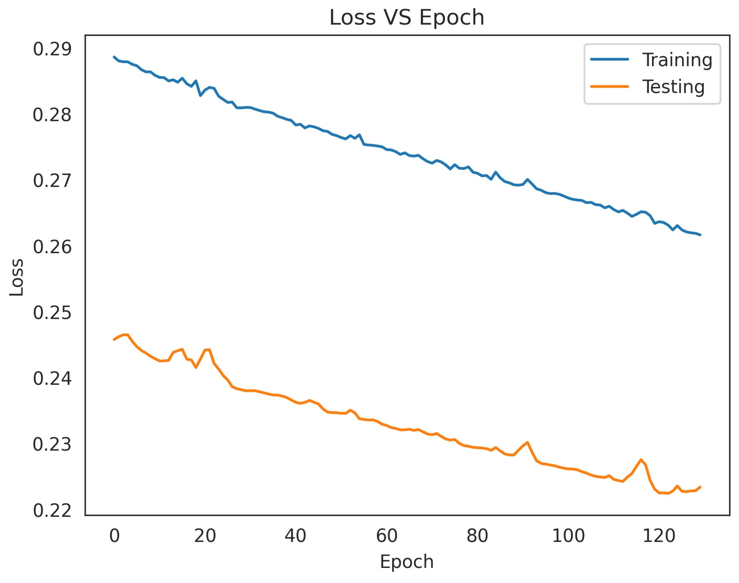
ANNs are composed of multiple nodes that resemble real brain neurons. The neurons are interconnected and interact with one another. The nodes can take data as input and perform basic operations on them. A neuron’s processing component receives numerous signals. Sometimes, signals are altered at the receiving synapses, and the processing element adds the weighted inputs. The output of a neuron is the result of a threshold activation function. If the threshold is crossed, the process is repeated and the signal becomes an input to other neurons [22,23]. Figure 4 shows the sequential model that we used. The neural net was trained for 130 epochs. When a greater number of neurons are used in the hidden layer, the chances of overfitting the data increase, as an ANN memorizes more detailed features. For our model, we used 2 hidden layers with 128 and 32 nodes, respectively. The activation function for all the layers, except the last layer, was ReLU, while Tanh was used for the last layer. To reduce the loss during back-propagation and improve the efficiency, an AdaMax optimizer was used.

2.3.5. Approach Used to Carry Out ML

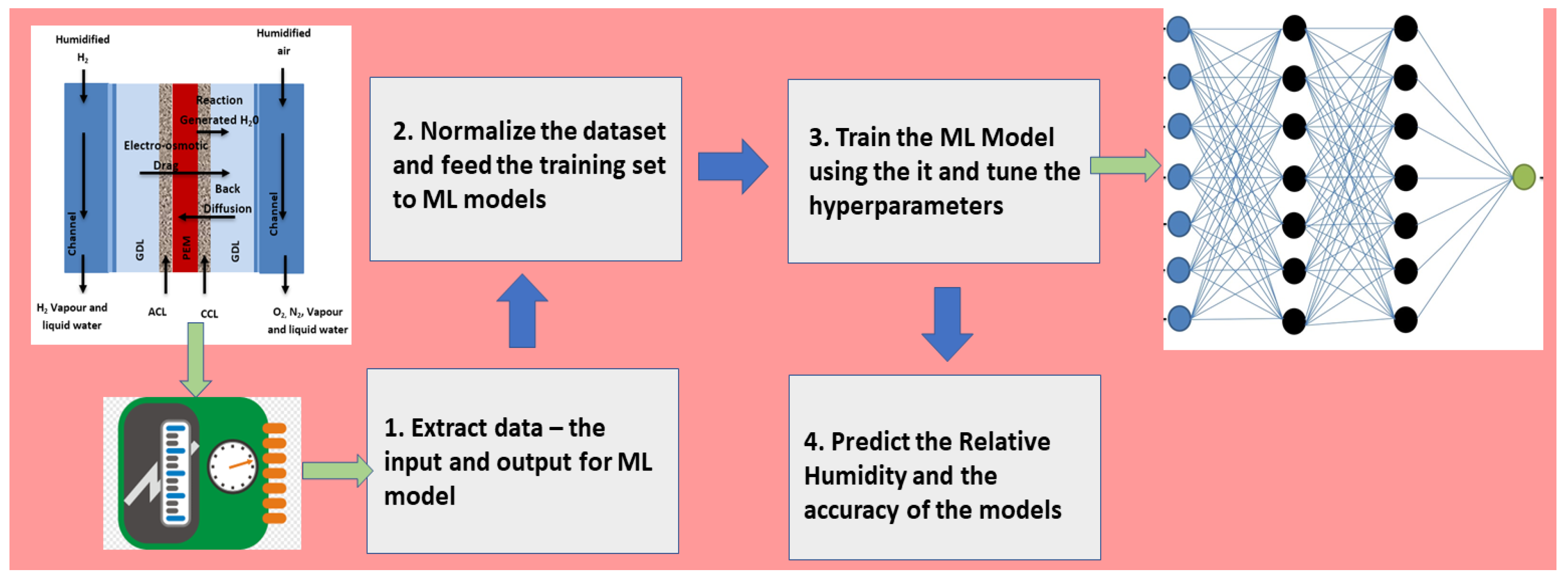
The dataset was first scaled before feeding it to the ML models (Figure 5). After scaling, a heat map was plotted to determine the correlation among the parameters. Then, the dataset was split into an 80:20 ratio, whereby 80% of the randomly selected points were used as a training set for the models, and the remaining 20% of the data points were used as testing set for the models. The hyperparameters and kernel function of the models were fine-tuned using the GridSearchCV v1,3 function, and the best-fit values were input into the model [24]. Table 3 shows the various hyperparameter values obtained using GridSearchCV. These models were trained with the training set and, finally, the accuracy of the models was calculated using the test set. This accuracy of all four models (SVM, DT, RF, and ANN) was then found using various matrices, such as R squared (R2), mean squared error (MSE), root mean square error (RMSE) and mean absolute error (MAE). To ensure that there was no overfitting of the models a 10-fold cross-validation was used, and it was observed that the value of the 10 folds matched the accuracy of all of the models. The results for these models are displayed in Table 3, and a comparison of all of the model accuracies is also shown.

3. Results and Discussions

3.1. Analyzing the Dehydration and Flooding in the Cell

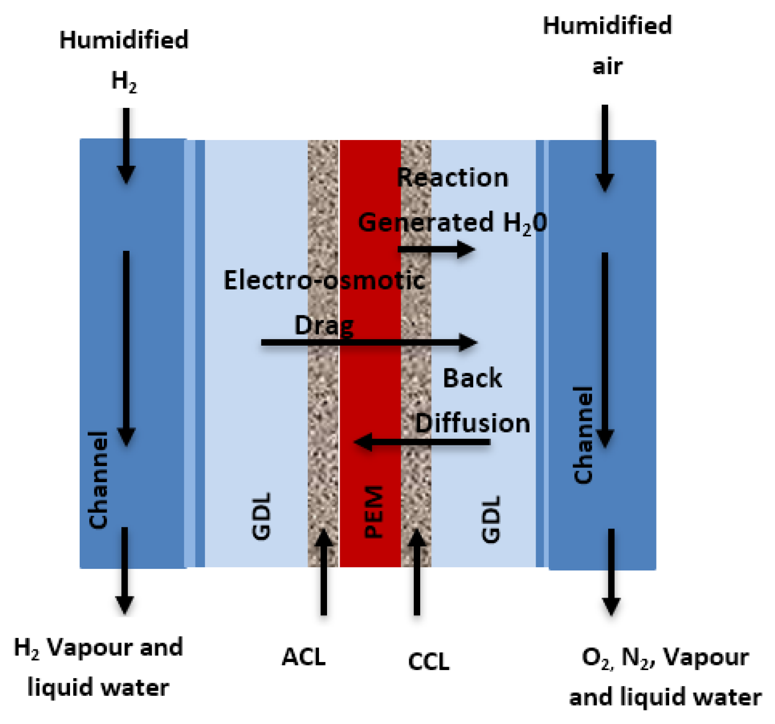
The problem of dehydration or flooding arises because of different water transport mechanisms in a cell, which include the back diffusion of water from the cathode to the anode, the electro-osmotic drag from the anode to the cathode, and the convective transfer brought on by pressure gradients within the fuel cell stack. The cathode’s performance acts as a limiting factor for the fuel cell’s performance, as the kinetics of the ORR is 4–6 times lower in magnitude than the hydrogen evolution reaction (HOR); thus, the ORR is the rate-determining step. Water is carried by protons as they move from the anode to the cathode through the electrolyte membrane, causing electro-osmotic drag. Back diffusion is the only process by which the cathode loses water. However, this process moves much more slowly than the water produced by ORRs and electro-osmotic drag. Figure 6 shows the various pathways for the flow of water. As a result, it is crucial to periodically or continuously remove water. Excess water will build up if the rate of removal is lower than the rates of generation and drag (especially near the cathode), resulting in flooding [25,26,27].
Conversely, membrane dehydration occurs when the rate of water removal exceeds the rates of water creation and electro-osmotic drag. This can also lead to PEMFCs performing poorly, since it weakens the polymer and increases ohmic losses as a result of the membrane’s electrical resistance significantly increasing. Because of the dehydration, the overpotential of the anode and cathode increases significantly. The effects of dehydration are permanent, and even after rehydration, high ionic and contact resistances persist. The water in a PEM needs to be maintained adequately for the optimum operation of the fuel cell. It should be in equilibrium with the membrane to maximize the conductivity [28,29,30]. The ionic conductivity, water activity and membrane resistance can be regained when the cell is rehydrated. Hotspots and pinholes can occur when the cell is in the dry (i.e., dehydration) mode for longer periods. In such cases, recovering the ion conductivity is unlikely, as the membrane could be damaged. A Nafion membrane has a limited temperature window and operating regime (60–80 °C) with which to regain its ionic property when it is rehydrated. Regaining the performances of the hydrocarbon and the composite-based membrane is only possible if the membrane is rehydrated or soaked in acid between cycles. However, the rehydration mechanism in these cells is not well understood.

3.2. Importance of Relative Humidity in Flooding and Dehydration Predication

Fuel cells are used under various climatic conditions. Especially at very high temperatures, there is a need to maintain the humidity (RH > 80) of the cell for normal working conditions. The RH affects the cathode side significantly because of the presence of condensed water during the electrochemical reaction at the cathode side. Various studies conducted on the effect of the RH on a cell’s performance have found that reducing the RH in the cell results in the membrane resistance increasing, proton activity in the catalyst decreasing, platinum utilization decreasing, electrode kinetics decreasing and gas mass transfer resistance increasing, thereby reducing the efficiency of the cell [13,31,32,33,34]. Contrary to this, if the relative humidity of the cell increases to a particular point, in that case it would lead to the condensation of the excess vapor and the formation of a water layer on the electrodes, which could lead to flooding. Thus, the RH plays an important role in determining dehydration or flooding in the cell.
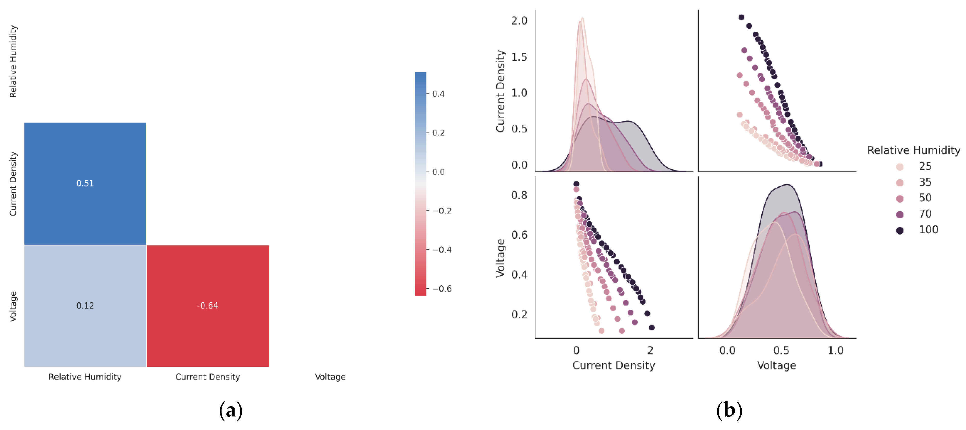
Further, for our model a heat map (Figure 7) was also plotted to show the numerical relationship between the various parameters and also to visualize trends in the data. The results show that the water distribution has a strong positive relationship with the current density, which is also evident from the above heat map.
The conventional method used for determining the relative humidity of a cell is time-consuming, as it involves an elaborate experimental set-up [15]. Our data-driven model can, thus, be used to predict the relative humidity of a cell based on the current density and voltage. ML models can approximate any nonlinear relationship in a high dimensional space; they can be used to understand the intricate connections among a fuel cell system’s variables, which are challenging to express using straightforward mathematical equations. An analysis of the relative humidity can be conducted to determine the condition under which dehydration or flooding occurs in the fuel cell. Based on the results of an ML model, appropriate steps can immediately be taken to prevent a further loss of efficiency in the case of an abnormality in the working conditions. The greatest advantage of this method is the computational speed in analyzing the results, as once an ML model is trained, it can be used for real-time application and make accurate predictions in situations where time is a major factor, such as when the loss of efficiency or the late detection of such factors could gravely impact the membrane and cathode. The efficiency of these models can be further increased if we take into consideration additional factors, which we plan to do in the future.

3.3. Comparison of Machine Learning Models

To quantify and assess the accuracy of the machine learning models, various matrices (measures) were used. The metrics included R squared (R2), mean squared error (MSE), root mean square error (RMSE) and mean absolute error (MAE) [35,36,37].
The R-squared error establishes the percentage of the dependent variable’s variance that the independent variable may account for.
R 2 = 1 S S R S S M
where SSR is the sum of the squared errors of the regression line, and SSM is the sum of the squared error of the mean line.
The mean squared error measures the average squared difference between the estimated and actual values.
M S E = 1 n i = 1 n ( Y i Y p ) 2
The root mean square error is a measure of the spread of data around the best-fit line.
R M S E = i = 1 n ( Y i Y p ) 2 n
The mean absolute error is the average of the absolute values of the individual prediction errors for all instances in the dataset.
M A E = i = 1 n | Y p Y i | n
where n stands for the total number of data points, Yi is the observed value and Yp is the predicted value.
Decision trees are built based on algorithms (e.g., Hunt’s algorithm) that determine an optimal choice at each node. The algorithms tend to make the most optimal decision at each step rather than accounting for a global optimum. However, selecting the best outcome at each step does not guarantee the model will be travelling in the direction that will result in the best choice when it reaches the leaf node, the tree’s final node. Thus, a decision tree’s algorithm has a lower efficiency than other models, which was evident in our results. Random forest models are a robust modeling approach and better than decision tree, as they combine several decision trees to reduce overfitting and bias-related inaccuracy, producing beneficial results. SVM, DT and RF undergo single-step training once the data are fed to these models (Figure 8). An ANN, on the other hand, undergoes an iterative training process.
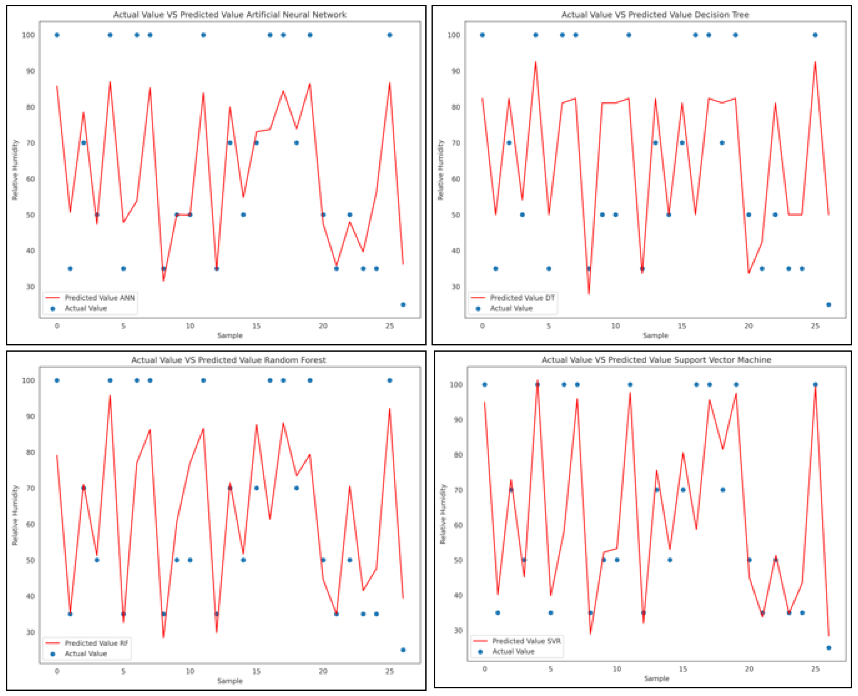
Figure 9 shows a graph plotting the loss and number of epochs. We can observe that after 130 epochs, the graph exhibits a constant trend, i.e., there was no change in loss. So, training beyond 130 epochs only increases the computational time while keeping the accuracy of the prediction constant. Thus, to reduce the computational time, we trained the model for only 130 epochs. Here, we can observe that as the epochs increased, the loss decreased until it became constant. Even with a smaller number of samples, the model’s accuracy was satisfactory, which was validated using the various matrices. The prediction by the four models for 27 samples is shown below.
From Figure 10, it is evident that support vector regression had the best-fit line, which was also evident using the various metrics. For a larger dataset, an ANN is theoretically found to outperform other regression models, and thus, for larger datasets, an ANN model can be used [38]. The only pitfall is that it is more time-consuming to train than other models. Ensemble learning models can be a viable solution for time-dependent cases because of their innate ability to identify nonlinear trends and handle noise effectively.
Applicability and Limitations of the model
  • Since no parameters, except voltage and current, are needed to assess failures in a cell, the proposed model can be applicable to different compositions of the GDL of a PEMFC. It can provide a performance analysis for both the PEMFC and durability of the cell based on the datasets used to train the model;
  • The model can predict the cause and effect of failure modes and the performance of a cell. However, the model cannot accurately assess the failure mechanism of the individual components and interfaces of the cell;
  • The deep learning model and methods proposed for the dehydration or flooding diagnosis are universal for any GDL materials. It could be applicable for use in testing a cell, as well as stacking and analyzing the proposed failure modes;
  • Gathering a larger dataset to compare it with modified FCM and SMOTE algorithms can enhance the fault detection modes for RH cycling in PEMFC tests. However, this approach is beyond the scope of the present study;
  • This study involved many features in the diagnosis of dehydration and flooding. Noise in the dataset requires an extra tree classifier to initially identify redundant features. Therefore, feature selection must be performed to reduce the computational cost and time. This is carried out before training the model. The regression approach is adopted to identify and alert for flooding- or dehydration-induced faults in a cell.

4. Conclusions

This study demonstrated the development of supervised learning and deep learning data-driven models using support vector machine, decision tree, random forest, and artificial neural networks modeling approaches. Models were developed based on data for current density, voltage and relative humidity obtained from the literature. The results were validated using 27 data points used as a testing set. The support vector regression model developed for the prediction of the relative humidity showed higher accuracy in comparison to other models. An ANN could also be used to predict the RH in the case of a larger dataset. ML models, being less time-consuming than the conventional method used for RH testing, can be used for the determination of the accurate precursors of dehydration or flooding, and appropriate water management techniques can be applied to prevent failure during the operation of a PEM under various conditions.

Author Contributions

Methodology, J.C.Z. and S.R.D.; Software, C.R.K.; Validation, J.T.; Formal analysis, J.C.Z.; Investigation, S.R.D. and C.R.K.; Resources, S.R.D. and M.M.; Data curation, J.C.Z.; Writing—draft, S.R.D.; Writing—review & editing, S.R.D.; Visualization, M.M.; Supervision, S.R.D. and J.T.; Project administration, M.M. and B.W. All authors have read and agreed to the published version of the manuscript.

Funding

This research received no external funding.

Data Availability Statement

Data are confidential.

Conflicts of Interest

The authors declare no conflict of interest.

Nomenclature

PEMFCPolymer electrolyte membrane fuel cell
MLMachine learning
GDLGas diffusion layer
ANNArtificial neural network
RFRandom forest
DTDecision tree
SVMSupport vector machine
RHRelative humidity
ORROxygen reduction reaction
FCMFuzzy C means algorithm
SMOTESynthetic minority oversampling technique
R2R squared (correlation coefficient)
MSEMean squared
RMSERoot mean square error
MAEMean absolute error
YiObserved value
YpPredicted value
CFDComputational fluid dynamics

References

  1. Li, T.; Wang, K.; Wang, J.; Liu, Y.; Han, Y.; Xu, Z.; Lin, G.; Liu, Y. Optimization of GDL to improve water transferability. Renew. Energy 2021, 179, 2086–2093. [Google Scholar] [CrossRef]
  2. Raman, S.; Iyeswaria, K.B.; Narasimhan, S.; Rengaswamy, R. Effects of water induced pore blockage and mitigation strategies in low temperature PEM fuel cells—A simulation study. Int. J. Hydrogen Energy 2017, 42, 23799–23813. [Google Scholar] [CrossRef]
  3. Springer, T.E.; Zawodzinski, T.A.; Gottesfeld, S. Polymer Electrolyte Fuel Cell Model. J. Electrochem. Soc. 1991, 138, 2334–2342. [Google Scholar] [CrossRef]
  4. Bernardi, D.M.; Verbrugge, M.W. A Mathematical Model of the Solid-Polymer-Electrolyte Fuel Cell. J. Electrochem. Soc. 1992, 139, 2477–2491. [Google Scholar] [CrossRef]
  5. Bednarek, T.; Tsotridis, G. Issues associated with modelling of proton exchange membrane fuel cell by computational fluid dynamics. J. Power Sources 2017, 343, 550–563. [Google Scholar] [CrossRef]
  6. Williams, M.V.; Kunz, H.R.; Fenton, J.M. Analysis of Polarization Curves to Evaluate Polarization Sources in Hydrogen/Air PEM Fuel Cells. J. Electrochem. Soc. 2005, 152, A635. [Google Scholar] [CrossRef]
  7. Pourrahmani, H.; van Herle, J. Water management of the proton exchange membrane fuel cells: Optimizing the effect of microstructural properties on the gas diffusion layer liquid removal. Energy 2022, 256, 124712. [Google Scholar] [CrossRef]
  8. Cawte, T.; Bazylak, A. A 3D convolutional neural network accurately predicts the permeability of gas diffusion layer materials directly from image data. Curr. Opin. Electrochem. 2022, 35, 101101. [Google Scholar] [CrossRef]
  9. Chauhan, V.; Mortazavi, M.; Benner, J.Z.; Santamaria, A.D. Two-phase flow characterization in PEM fuel cells using machine learning. Energy Rep. 2020, 6, 2713–2719. [Google Scholar] [CrossRef]
  10. Yu, Y.; Chen, S. Numerical study and prediction of water transfer in gas diffusion layer of proton exchange membrane fuel cells under vibrating conditions. Int. J. Energy Res. 2022, 46, 18781–18795. [Google Scholar] [CrossRef]
  11. Dhanushkodi, S.R. Experimental Methods and Mathematical Models to Examine Durability of Polymer Electrolyte Membrane Fuel Cell Catalysts. Ph.D. Thesis, University of Waterloo, Waterloo, ON, Canada, 2013. Available online: http://hdl.handle.net/10012/7619 (accessed on 1 May 2023).
  12. Zhang, J.; Tang, Y.; Song, C.; Xia, Z.; Li, H.; Wang, H.; Zhang, J. PEM fuel cell relative humidity (RH) and its effect on performance at high temperatures. Electrochim. Acta 2008, 53, 5315–5321. [Google Scholar] [CrossRef]
  13. Saleh, M.M.; Okajima, T.; Hayase, M.; Kitamura, F.; Ohsaka, T. Exploring the effects of symmetrical and asymmetrical relative humidity on the performance of H2/air PEM fuel cell at different temperatures. J. Power Sources 2007, 164, 503–509. [Google Scholar] [CrossRef]
  14. Sahu, I.P.; Krishna, G.; Biswas, M.; Das, M.K. Performance Study of PEM Fuel Cell under Different Loading Conditions. Energy Procedia 2014, 54, 468–478. [Google Scholar] [CrossRef]
  15. Kim, K.-H.; Lee, K.-Y.; Lee, S.-Y.; Cho, E.; Lim, T.-H.; Kim, H.-J.; Yoon, S.P.; Kim, S.H.; Lim, T.W.; Jang, J.H. The effects of relative humidity on the performances of PEMFC MEAs with various Nafion® ionomer contents. Int. J. Hydrogen Energy 2010, 35, 13104–13110. [Google Scholar] [CrossRef]
  16. Gunn, S.R. Support vector machines for classification and regression. ISIS Tech. Rep. 1998, 14, 5–16. [Google Scholar]
  17. Trafalis, T.B.; Ince, H. Support vector machine for regression and applications to financial forecasting. In Proceedings of the IEEE-INNS-ENNS International Joint Conference on Neural Networks, IJCNN 2000, Neural Computing: New Challenges and Perspectives for the New Millennium, Como, Italy, 27–27 July 2000; IEEE: Piscataway, NJ, USA, 2000; Volume 6. [Google Scholar]
  18. Pekel, E. Estimation of soil moisture using decision tree regression. Theor. Appl. Climatol. 2020, 139, 1111–1119. [Google Scholar] [CrossRef]
  19. Xu, M.; Watanachaturaporn, P.; Varshney, P.K.; Arora, M.K. Decision tree regression for soft classification of remote sensing data. Remote Sens. Environ. 2005, 97, 322–336. [Google Scholar] [CrossRef]
  20. Wang, L.; Zhou, X.; Zhu, X.; Dong, Z.; Guo, W. Estimation of biomass in wheat using random forest regression algorithm and remote sensing data. Crop J. 2016, 4, 212–219. [Google Scholar] [CrossRef]
  21. Liu, Y.; Wang, Y.; Zhang, J. New machine learning algorithm: Random forest. In Information Computing and Applications, Proceedings of the Third International Conference, ICICA 2012, Chengde, China, 14–16 September 2012; Springer: Berlin/Heidelberg, Germany, 2012. [Google Scholar]
  22. Setiono, R.; Leow, W.K.; Zurada, J.M. Extraction of rules from artificial neural networks for nonlinear regression. IEEE Trans. Neural Netw. 2002, 13, 564–577. [Google Scholar] [CrossRef]
  23. Asiltürk, I.; Çunkaş, M. Modeling and prediction of surface roughness in turning operations using artificial neural network and multiple regression method. Expert Syst. Appl. 2011, 38, 5826–5832. [Google Scholar] [CrossRef]
  24. Ambesange, S.; Vijayalaxmi, A.; Sridevi, S.; Venkateswaran; Yashoda, B.S. Multiple heart diseases prediction using logistic regression with ensemble and hyper parameter tuning techniques. In Proceedings of the 2020 Fourth World Conference on Smart Trends in Systems, Security and Sustainability (WorldS4), London, UK, 27–28 July 2020; IEEE: Piscataway, NJ, USA, 2020. [Google Scholar]
  25. Carton, J.G.; Lawlor, V.; Olabi, A.G.; Hochenauer, C.; Zauner, G. Water droplet accumulation and motion in PEM (Proton Exchange Membrane) fuel cell mini-channels. Energy 2012, 39, 63–73. [Google Scholar] [CrossRef]
  26. Afra, M.; Nazari, M.; Kayhani, M.H.; Sharifpur, M.; Meyer, J.P. 3D experimental visualization of water flooding in proton exchange membrane fuel cells. Energy 2019, 175, 967–977. [Google Scholar] [CrossRef]
  27. Zhang, J.; Li, H.; Shi, Z.; Zhang, J. Effects of hardware design and operation conditions on PEM fuel cell water flooding. Int. J. Green Energy 2010, 7, 461–474. [Google Scholar] [CrossRef]
  28. Laribi, S.; Mammar, K.; Sahli, Y.; Koussa, K. Analysis and diagnosis of PEM fuel cell failure modes (flooding & dehydration) across the physical parameters of electrochemical impedance model: Using neural networks method. Sustain. Energy Technol. Assess. 2019, 34, 35–42. [Google Scholar]
  29. Debenjak, A.; Gasperin, M.; Pregelj, B.; Atanazijevič-Kunc, M.; Petrovčič, J.; Jovan, V. Detection of Flooding and Dehydration inside a PEM Fuel Cell Stack. Stroj. Vestn./J. Mech. Eng. 2013, 59, 56–64. [Google Scholar] [CrossRef]
  30. Brèque, F.; Ramousse, J.; Dubé, Y.; Agbossou, K.; Adzakpa, P. Sensibility study of flooding and dehydration issues to the operating conditions in PEM Fuel Cells. Int. J. Energy Environ. IJEE 2010, 1, 1–20. [Google Scholar]
  31. Xu, H.; Kunz, H.R.; Fenton, J.M. Analysis of proton exchange membrane fuel cell polarization losses at elevated temperature 120 °C and reduced relative humidity. Electrochim. Acta 2007, 52, 3525–3533. [Google Scholar] [CrossRef]
  32. Jiang, R.; Kunz, H.R.; Fenton, J.M. Influence of temperature and relative humidity on performance and CO tolerance of PEM fuel cells with Nafion®–Teflon®–Zr (HPO4)2 higher temperature composite membranes. Electrochim. Acta 2006, 51, 5596–5605. [Google Scholar] [CrossRef]
  33. Abe, T.; Shima, H.; Watanabe, K.; Ito, Y. Study of PEFCs by AC impedance, current interrupt, and Dew point measurements: I. Effect of humidity in oxygen gas. J. Electrochem. Soc. 2003, 151, A101. [Google Scholar] [CrossRef]
  34. Broka, K.; Ekdunge, P. Oxygen and hydrogen permeation properties and water uptake of Nafion® 117 membrane and recast film for PEM fuel cell. J. Appl. Electrochem. 1997, 27, 117–123. [Google Scholar] [CrossRef]
  35. Chai, T.; Draxler, R.R. Root mean square error (RMSE) or mean absolute error (MAE)?–Arguments against avoiding RMSE in the literature. Geosci. Model Dev. 2014, 7, 1525–1534. [Google Scholar] [CrossRef]
  36. Allen, D.M. Mean square error of prediction as a criterion for selecting variables. Technometrics 1971, 13, 469–475. [Google Scholar] [CrossRef]
  37. Cameron, A.C.; Windmeijer, F.A.G. An R-squared measure of goodness of fit for some common nonlinear regression models. J. Econ. 1997, 77, 329–342. [Google Scholar] [CrossRef]
  38. Lee, K.-Y.; Kim, K.-H.; Kang, J.-J.; Choi, S.-J.; Im, Y.-S.; Lee, Y.-D.; Lim, Y.-S. Comparison and analysis of linear regression & artificial neural network. Int. J. Appl. Eng. Res. 2017, 12, 9820–9825. [Google Scholar]
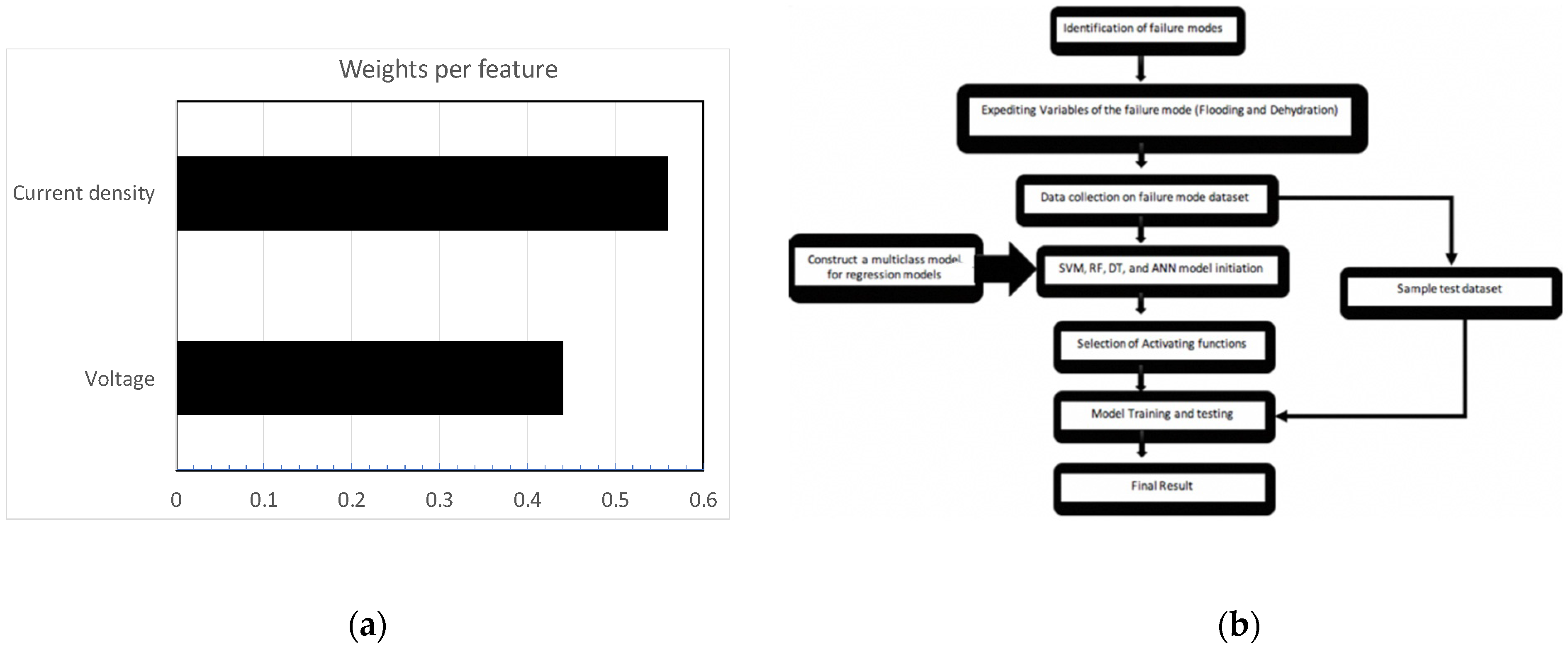
Figure 1. (a) Feature selection using the extra trees classifier, which assigns an importance score for each feature, and the feature with the highest score affects the output the most significantly; (b) generic modeling approach.
Energies 16 06968 g001
Figure 2. Structure of our decision tree model visualizing how a decision is made in the prediction of an output.
Energies 16 06968 g002
Figure 3. Last decision tree out of the 350 trees in our random forest. The tree has been split into four parts (ad) to describe the details related to the decision tree regression.
Energies 16 06968 g003aEnergies 16 06968 g003b
Figure 4. Sequential ANN model used in our study. Here, the two hidden layers are shown. The circles marked with green show the input into the ANN model, while the circle marked with red shows the output of the ANN model.
Energies 16 06968 g004
Figure 5. Procedure followed to develop the ML models.
Energies 16 06968 g005
Figure 6. Pathways for water transport in a PEM fuel cell.
Energies 16 06968 g006
Figure 7. Heat map and plots showing the bivariant distribution of the dataset. (a) Two-dimensional form using Voltage and current density in different colors to show different data values vary with RH, and (b) Correlation of polarization curve at different RH with bivariant distribution.
Energies 16 06968 g007
Figure 8. Histogram comparing the four models.
Energies 16 06968 g008
Figure 9. Graph comparing the loss and number of epochs.
Energies 16 06968 g009
Figure 10. Prediction of the four models for 27 samples.
Energies 16 06968 g010
Table 1. Literature findings.
Models and MethodFindings and Research NeedsReference
Artificial neural networkMaximum liquid removal by the GDL was predicted using permeability and porosity as inputs.[7]
Convolution neural networkThe permeability of the gas diffusion layer was predicted.[8]
Logistic regression, artificial Neural network and support vector machineTwo-phase flow pressure drops in the flow channel of the PEM were classified into three categories using ML.[9]
Genetic algorithm–back propagation neural networkPrediction of water saturation in the GDL.[10]
Table 2. Visualization of the dataset used for training.
IndexRelative HumidityCurrent DensityVoltage
133133133
Mean60.451127820.5458657910.495899594
Std.28.480845810.4952564460.186822813
Min.00.003955020.11413
25%350.1710830.358696
50%500.3694740.505435
75%1000.822040.63587
Max.1002.03890.9491952
Table 3. Various hyperparameter values used in the models.
ModelHyperparameter Value
Support vector regressionKernelRBF
C14
Decision treeMax_depth5
Min_sample_leaf2
min_weight_fraction_leaf0.1
Artificial neural networkOptimizerAdamax
lossMean-square-error
ActivationReLU (for Input and hidden layer)
Tanh (for output)
Hidden Layer2
Disclaimer/Publisher’s Note: The statements, opinions and data contained in all publications are solely those of the individual author(s) and contributor(s) and not of MDPI and/or the editor(s). MDPI and/or the editor(s) disclaim responsibility for any injury to people or property resulting from any ideas, methods, instructions or products referred to in the content.