Research on an Improved Carbon Emission Flow Model Considering Electric Vehicle Charging Fluctuation and Hybrid Power Transaction

Abstract

With the update of the power transaction mode and the access of increasing electric vehicles with high randomness to the power grid, the existing carbon emission flow calculation method cannot consider the influence of carbon emission due to the fluctuation in electric vehicle charging and various transaction modes. Given the above shortcomings, this paper proposes an improved carbon emission flow model considering electric vehicle charging fluctuations and hybrid power transactions. The model first considers different transaction modes, allocates the network loss to both sides of power generation, and forms a lossless network, realizing the decoupling of the bilateral transaction mode, pool transaction mode, and network loss and then calculating the day-ahead network’s carbon emission. Then, the changes in different transaction modes caused by the fluctuation in electric vehicle charging under different transaction modes are analyzed and the nodes of ‘spontaneous change’ are found to form a day-ahead intra-day deviation network and calculate its carbon emission flow. Finally, the calculation results are combined to obtain an improved power system carbon emission flow considering electric vehicle charging fluctuations and transaction modes. In this paper, the 33-node system is used for verification.

1. Introduction

To fulfill the “Paris Agreement” and gradually promote China’s environmental protection strategy [1], the Chinese government proposed a grand vision of “carbon peak” in 2030 and “carbon neutrality” in 2060 [2]. With the gradual advancement of the “double carbon” goal [3], an increasing number of electric vehicles (EVs) are connected to the power grid. Although it optimizes the industrial structure of China’s power grid and positively affects energy conservation and emission reduction, it puts forward higher requirements on balancing the power system’s stability and environmental protection [4].

The advent of a clean and efficient electric vehicle (EV) holds considerable promise in alleviating environmental and energy exigencies. However, EV’s stochastic, probabilistic, and uncertain nature engenders complex ramifications. As EVs proliferate and interface with the power grid substantially, a gamut of predicaments ensues, encompassing line congestion, exacerbated network dissipation, harmonic contamination, and perturbations in three-phase equilibrium. The collective impact of these variables impinges upon the power grid’s operational security and economic viability [5]. A comprehensive assessment of the ramifications associated with the grid integration of EVs underscores six cardinal dimensions: safety [6], reliability [7], economic prudence [8], harmonized coordination, operational efficiency, and power quality [9]. Extant scholarly inquiry, however, primarily gravitates toward the electrical attributes, commonly eschewing dynamic orchestration of EV users’ charging proclivities in congruence with temporal fluxes in carbon emissions.

In the existing studies, the calculation of carbon emission mainly includes the macro statistical method [10,11,12,13,14] and carbon flow analysis method [15,16]. The macro statistical practice is based on long-term macro data and calculates the total energy consumed within the required time scale (usually years). This method has the advantages of simple calculation, convenient use, and accurate results. Therefore, it is widely used in long-term carbon emission calculation [17]. Power flow tracking technology can be applied to calculate the network carbon flow under deterministic power flow [18,19] based on the proportional sharing assumption used in power flow tracking to track the active power flow. Based on graph theory, Ref. [20] proposed a complex power flow tracing method mainly used for no circulation. However, this method has apparent defects because the time granularity is too large, resulting in the poor real-time inability to describe the microscopic changes of various carbon indicators in detail [17]; it is difficult to track the specific flow of carbon emission accurately. The carbon flow analysis method [21] is based on the power flow calculation of the power system. According to the principle of ‘proportional allocation’, the power flowing through the grid is labeled as ‘carbon label’, which fully reflects the transfer of carbon emission flow in the whole process of power generation, transmission, transformation, and distribution to realize the accurate tracking and traceability of the specific flow direction of carbon emission [22]. Therefore, the carbon flow analysis method can monitor the flow of carbon emissions in the power network in real-time, which is not only conducive to the analysis of the distribution characteristics of carbon emission flow by power practitioners but also enables power users to clearly understand the carbon emission caused by their electricity consumption behavior [23], thus extensively promoting the development of carbon emission analysis and statistics in power systems [24,25,26].

Although the carbon flow analysis method has experienced many years of development and improvement, with the renewal of the electricity market transaction mode and the increasing number of EVs with high randomness, the calculation of carbon emission flow can not only stay in the static analysis of carbon emission flow but should be combined with the current situation of the power system. Therefore, the calculation of carbon emission flow is a new challenge. Currently, the electricity market is mainly divided into the pool transaction (PT) mode and bilateral transaction (BT) mode according to the transaction mode and there are usually hybrid electricity market transactions with PT and BT modes in the power network. Based on considering the influence of carbon trading and the demand side response, Ref. [27] proposed a low-carbon planning method for distribution networks with the goal of economic and environmental protection; Ref. [28] offers a calculation method of carbon emission flow considering different transaction modes. However, it still calculates the static carbon emission flow in the known grid and cannot assess the impact of high-randomness EVs on carbon emissions after they are connected to the grid. In the calculation of carbon emission flow in [29], the change in carbon emission flow under the fluctuation in power generation and consumption is considered. However, different power transaction modes cannot be decoupled and the change in carbon emission flow caused by the update of power transaction modes cannot be evaluated more comprehensively. Moreover, the coupling between the modes in the power system is complex and the above two algorithms cannot be superimposed. Therefore, the calculation of carbon emission flow will not be able to use the traditional ‘proportional sharing’ principle and a new carbon emission flow calculation method must be adopted.

This study proffers an enhanced model for carbon emission flow to address the existing research landscape void and leverage insights about power transaction modalities and the underpinning determinants of EV charging fluctuations. This model comprehensively integrates these dimensions, conferring heightened rationality upon the calculus of carbon emission dynamics. It enables EV users to experience the carbon emissions caused by changes in their behavior, guides the charging behavior of EV users according to the carbon emissions of electricity, promotes the consumption of new energy, and lays the foundation for the time-of-use price based on carbon emissions.

The paramount originality and contributions of this paper are threefold.

(1)

According to the characteristics of the BT mode and PT mode, a new network loss allocation method considering a hybrid power transaction mode is proposed. According to different transaction modes, different power flow results are decoupled to facilitate the analysis of carbon emission flow under different transaction modes;

(2)

Fully considering the high randomness of EV charging and the accuracy of generator output prediction, this paper first proposed the concept of a ‘spontaneous change’ node, and on this basis, a deviation network was established to determine the cause of the change in carbon emission flow and to provide guiding rules and directions for the future goal of energy saving and emission reduction;

(3)

Through the nonlinear relationship in the calculation process of carbon emission flow in power systems, this paper proposed an improved carbon emission flow model considering EV charging fluctuation and hybrid power transaction, which provides a theoretical basis for EV users’ new energy consumption and low-carbon behavior.

The rest of this paper is arranged as follows. Section 2 introduces the concept and principle of power flow tracing. Section 3 presents the day-ahead hybrid transaction network, the network loss allocation method under different transaction modes, and the day-ahead network carbon emission flow calculation model. On this basis, Section 4 compares the day-ahead and intra-day actual networks, finds the ‘spontaneous change’ node, establishes the deviation network, and finally finds the improved carbon emission flow model considering the charging fluctuation in EVs and hybrid power transactions. Section 5 takes the IEEE-33 nodes system as a case, introduces the research results of the improved carbon emission flow model considering the fluctuation in EV charging and hybrid power transactions, and analyzes the rationality and feasibility of the model proposed in this paper. Finally, the main conclusions of this paper are given in Section 6.

2. Power Flow Tracing

Carbon emissions are predominantly linked to active power. Nonetheless, when employing DC power flow, the influence of network losses on carbon emission distribution tends to be overlooked. Hence, in this segment, the approach initially segregates network losses from the outcomes of AC power flow, subsequently attributing them to both ends of the ‘source-load’. This step aims to configure a network devoid of losses. Later, deconstructing the DC power flow makes it possible to compute the carbon emission flow across various transaction modes.

2.1. Reverse Power Flow Tracing

For any node in the grid, the inflow power $P_i$ of node i can be known from the conservation of inflow power and outflow power as follows:

$$P_i={\displaystyle \sum _{j\in i^{-}}{P}_{ij}}+P_{Li}$$

(1)

where $i^{-}$ is the set of downstream nodes of node i; $P_{ij}$ is the power flowing out of node i on the branch ij; and $P_{Li}$ is the load on node i. If node i has no load, the variable is zero.

$P_{ij}$ in the above (1) can be changed into the sum of the power $\left|P_{ji}\right|$ injected into node j and the network loss $P_{ij,\mathrm{loss}}$ on branch ij. Then, (1) can be transformed into the following form:

$$P_i={\displaystyle \sum _{j\in i^{-}}\left|P_{ji}\right|}+P_{i^{-},\mathrm{loss}}+P_{Li}$$

(2)

where $P_{i^{-},\mathrm{loss}}$ is the sum of the network loss of all downstream node branches connected to node i; the above (2) can be rewritten as:

$$P_i-{\displaystyle \sum _{j\in i^{-}}\frac{\left|P_{ji}\right|}{P_j}\times }{P}_j=P_{i^{-},\mathrm{loss}}+P_{Li}$$

(3)

By transforming the above (3) into a matrix form, it can be expressed as:

$$A_{d}P=P_L+P_{{\mathsf{\Sigma }}^{-},\mathrm{loss}}$$

(4)

where $P_{{\mathsf{\Sigma }}^{-},\mathrm{loss}}$ is the network loss set on the branch composed of the downstream nodes of all nodes in the grid and P is the vector consisting of the injection power of all nodes in the grid. $P_L$ is the node load power vector and $A_d$ is the downstream distribution matrix and its elements are as follows:

$${\left[A_d\right]}_{ij}=\left\{\begin{array}{cc}\begin{array}{l}1\\ -\left|P_{ji}\right|/P_j\\ 0\end{array}& \begin{array}{l},j=i\\ ,j\in i^{-}\\ ,\mathrm{other}\end{array}\end{array}\right.$$

(5)

Assuming that the injection power on the generator node i in the network is $S_{\mathrm{G}i}$, the parameter can be rewritten as follows:

$$P_{\mathrm{G}i}=\frac{P_{\mathrm{G}i}}{P_i}{P}_i=\frac{P_{\mathrm{G}i}}{P_i}{e}_i^{\mathrm{T}}P=\frac{P_{\mathrm{G}i}}{P_i}{e}_i^{\mathrm{T}}{A}_d^{-1}\left(P_L+P_{{\mathsf{\Sigma }}^{-},\mathrm{loss}}\right)$$

(6)

where $e_i^{\mathrm{T}}\in R^n$ is the column vector whose i variable is one and the remaining variables are zero (the same below) and n is the number of nodes in the grid. According to (6), the network loss caused by generator node i is $P_{\mathrm{G}i,\mathrm{loss}}$:

$$P_{\mathrm{G}i,\mathrm{loss}}=\frac{P_{\mathrm{G}i}}{P_i}{e}_i^{\mathrm{T}}{A}_d^{-1}{P}_{{\mathsf{\Sigma }}^{-},\mathrm{loss}}$$

(7)

2.2. Forward Power Flow Tracing

This paper uses the forward power flow tracing method to solve the power absorbed by the load and branch in the grid with each generator. Like the reverse power flow tracing method, the upstream distribution matrix $A_u$ can be obtained as follows:

$${\left[A_u\right]}_{ij}=\left\{\begin{array}{cc}\begin{array}{l}1\\ -\left|P_{ji}\right|/P_i\\ 0\end{array}& \begin{array}{l},i=j\\ ,i\in j^{+}\\ ,\mathrm{other}\end{array}\end{array}\right.$$

(8)

According to the upstream distribution matrix $A_u$, the power absorbed by the load and the branch from the generator can be obtained.

$$\left\{\begin{array}{l}{P}_{\mathrm{L}k,\mathrm{G}i}=\frac{P_{\mathrm{L}k}{P}_{\mathrm{G}i}}{P_k}{e}_k^{\mathrm{T}}{A}_u^{-1}{e}_i\\ S_{kj,\mathrm{G}i}=\frac{P_{kj}{P}_{\mathrm{G}i}}{P_k}{e}_k^{\mathrm{T}}{A}_u^{-1}{e}_i\end{array}\right.$$

(9)

where $P_{\mathrm{L}k,\mathrm{G}i}$ is the power absorbed by the load node k on the generator node i; $P_{kj,\mathrm{G}i}$ is the power absorbed by the branch kj on the generator node i; $P_{\mathrm{L}k}$ is the load on the load node k; and $P_{kj}$ is the power flow on branch kj.

If we want to calculate the network loss on the load side, a virtual generator node can be established on each branch. The injected power to the grid is the opposite number of the branch loss and the network loss borne by the corresponding load can be obtained by the forward power flow tracing method. The specific calculation method is shown in [29], which is not repeated in this paper.

3. Day-Ahead Network Carbon Emission Flow Calculation Method

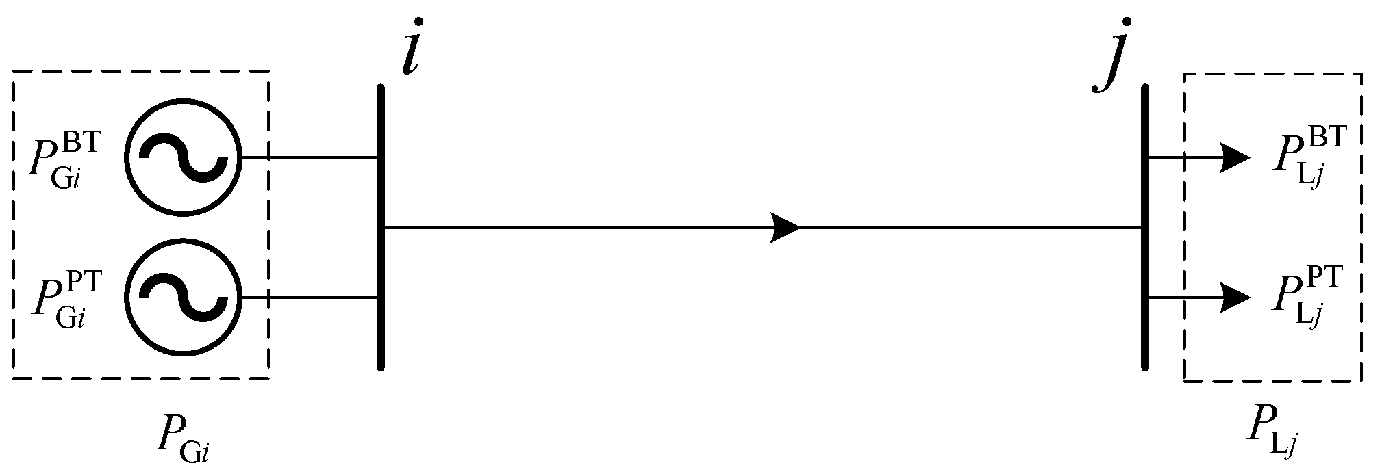
3.1. Day-Ahead Hybrid Transaction Network

When splitting the network according to different transaction modes, the following three principles should be met:

(1).

Load demand in BT mode: When calculating the load demand in the day-ahead BT mode, increasing the amount of network loss allocated in the BT is necessary under the premise of the original demand;

(2).

Power generation in the BT mode: When calculating the power generation in the day-ahead BT mode, the network loss allocated by the power plant does not need to be modeled by exceptional splitting but only needs to match the load demand after being transformed into a lossless network;

(3).

Power generation and load under the PT mode: To meet the overall power generation and load, subtract the power generation and load after the split in the BT mode.

3.2. Day-Ahead Lossless Network

Since BT can only involve specific power plants and users, when calculating the carbon emission involved in BT, they should not be calculated together with the irrelevant nodes. Therefore, distinguishing whether network losses belong to BT or PT is a problem to be solved in this section.

This paper takes the simple system shown in Figure 1 as an example. In the figure, both the generator and load participate in BT and PT at the same time, as shown in the following figure:

As illustrated in Figure 1, the generator node retains its fundamental nodal attributes due to the sole division of power. Consequently, the carbon emission intensity remains unaltered, leading to the preservation of the carbon emission flow after node division. However, (7) reveals a nonlinear relationship between the injected power of the generator and the resultant network loss it induces. This intricacy precludes a linear apportionment of network loss among diverse transactions based on power supply ratios. To delve into this matter, the subsequent analysis delves into the dynamics of network loss, along with the corresponding construct of a day-ahead lossless network, across two distinct transaction modes:

3.2.1. Network Loss and Its Day-Ahead Lossless Network under BT Mode

Network Loss of the BT Mode

In the actual power flow calculation, the power injected by the generator units participating in the BT does not necessarily flow into the load node with which the prescribed flow direction signs the contract. The transaction path is not necessarily equal to the power flow path but the network loss caused by participating in the BT on the load side is actual. Therefore, this paper believes that when calculating the network loss of BT, we should start from the load side and allocate the network loss calculated by the load side to both sides of BT according to a certain proportion. From the forward power flow tracing method described in Section 2.2, the network loss caused by each load node participating in the BT can be obtained, as shown in (10):

$$P_{\mathrm{L}j,\mathrm{loss}}^{\mathrm{BT}}=-{\displaystyle \sum _{j=n_b+1}^{n_b+n_l}\frac{P_{\mathrm{L}j}^{\mathrm{BT}}{P}_{\mathrm{G}i}^{\mathrm{loss}}}{P_j}{e}_j^{\mathrm{T}}{A^{\prime }}_u^{-1}{e}_i}$$

(10)

where $P_{\mathrm{L}j,\mathrm{loss}}^{\mathrm{BT}}$ is the network loss caused by the load node j participating in the BT part and $n_b$ and $n_l$ are the number of nodes and branches in the grid, respectively. ${{\mathit{A}}^{\prime }}_u$ increases the upstream distribution matrix of virtual generator nodes and $P_{\mathrm{G}i}^{\mathrm{loss}}$ is the virtual generator node of the branch.

Day-Ahead Lossless Network of the BT Mode

Generators and loads involved in BT should be converted as follows:

$$\left\{\begin{array}{l}{P}_{\mathrm{L}j}^{\mathrm{BT},\mathrm{after}}=P_{\mathrm{L}j}^{\mathrm{BT}}+\left(1-{\delta }^{\mathrm{BT}}\right)P_{\mathrm{L}j,\mathrm{loss}}^{\mathrm{BT}}\\ P_{\mathrm{G}i}^{\mathrm{BT},\mathrm{after}}=P_{\mathrm{L}j}^{\mathrm{BT},\mathrm{after}}\\ P_{\mathrm{G}i}^{\mathrm{BT}}=P_{\mathrm{G}i}^{\mathrm{BT},\mathrm{after}}+{\delta }^{\mathrm{BT}}{P}_{\mathrm{L}j,\mathrm{loss}}^{\mathrm{BT}}\end{array}\right.$$

(11)

where $P_{\mathrm{G}i}^{\mathrm{BT},\mathrm{after}}$ and $P_{\mathrm{L}j}^{\mathrm{BT},\mathrm{after}}$ are the generator and load power after being transformed into a lossless network in the BT mode and ${\delta }^{\mathrm{BT}}$ is the proportion of BT network loss borne by generators. This paper defines it as average allocation, so ${\delta }^{\mathrm{BT}}$ = 0.5. Subsequently, the specific value of ${\delta }^{\mathrm{BT}}$ can be set according to different allocation requirements according to the analytic hierarchy process and other methods.

3.2.2. Network Loss and Its Day-Ahead Lossless Network under the PT Mode

Network Loss of the PT Mode

Unlike the BT network, the PT mode only needs to meet the primary flow constraints and there is no specified flow direction. Therefore, the transaction path is the same as the power flow path in the PT mode. Therefore, in the PT, the status of each node is equal and the network loss of the PT undertaken by the generator node and the load node is shown in (12) and (13):

$$\left\{\begin{array}{ll}{P}_{\mathrm{G}i,\mathrm{loss}}^{\mathrm{PT}}={\delta }^{\mathrm{PT}}\frac{P_{\mathrm{G}i}}{P_i}{e}_i^{\mathrm{T}}{A}_d^{-1}& P_{{\mathsf{\Sigma }}^{-},\mathrm{loss}}\\ & ,\hspace{0.33em}\mathrm{if}\hspace{0.33em}i\notin N^{\mathrm{BT}}\\ P_{\mathrm{G}i,\mathrm{loss}}^{\mathrm{PT}}={\delta }^{\mathrm{PT}}\frac{P_{\mathrm{G}i}}{P_i}{e}_i^{\mathrm{T}}{A}_d^{-1}& P_{{\mathsf{\Sigma }}^{-},\mathrm{loss}}-{\delta }^{\mathrm{BT}}{P}_{\mathrm{L}j,\mathrm{loss}}^{\mathrm{BT}}\\ & ,\hspace{0.33em}\mathrm{if}\hspace{0.33em}i\in N^{\mathrm{BT}}\end{array}\right.$$

(12)

$$\left\{\begin{array}{ll}{P}_{\mathrm{L}j,\mathrm{loss}}^{\mathrm{PT}}=& \\ \hspace{0.33em}\hspace{0.33em}\hspace{0.33em}-\left(1-{\delta }^{\mathrm{PT}}\right){\displaystyle \sum _{k=n_b+1}^{n_b+n_l}}& \frac{P_{\mathrm{L}j}{P}_{\mathrm{G}i}^{\mathrm{loss}}}{P_k}{e}_k^{\mathrm{T}}{A^{\prime }}_u^{-1}{e}_i\\ & ,\hspace{0.33em}\mathrm{if}\hspace{0.33em}j\notin N^{\mathrm{BT}}\\ P_{\mathrm{L}j,\mathrm{loss}}^{\mathrm{PT}}=& \\ \hspace{0.33em}\hspace{0.33em}\hspace{0.33em}-\left(1-{\delta }^{\mathrm{PT}}\right){\displaystyle \sum _{j=n_b+1}^{n_b+n_l}}& \frac{P_{\mathrm{L}j}{P}_{\mathrm{G}i}^{\mathrm{loss}}}{P_j}{e}_j^{\mathrm{T}}{A^{\prime }}_u^{-1}{e}_i\\ \hspace{0.33em}\hspace{0.33em}\hspace{0.33em}-\left(1-{\delta }^{\mathrm{BT}}\right)P_{\mathrm{L}j,\mathrm{loss}}^{\mathrm{BT}}& \\ & ,\hspace{0.33em}\mathrm{if}\hspace{0.33em}j\in N^{\mathrm{BT}}\end{array}\right.$$

(13)

where $P_{\mathrm{G}i,\mathrm{loss}}^{\mathrm{PT}}$ and $P_{\mathrm{L}j,\mathrm{loss}}^{\mathrm{PT}}$ are the network loss of the PT undertaken by the generator node i and the load node j, respectively; ${\delta }^{\mathrm{PT}}$ is the proportion of the PT network loss borne by the generator and its value is the same as ${\delta }^{\mathrm{BT}}$; and $N^{\mathrm{BT}}$ is a set of nodes with BT.

Day-Ahead Lossless Network of the PT Mode

After obtaining the network loss shared by the two parties under the PT network, the day-ahead lossless PT network can be obtained, as shown in (14):

$$\left\{\begin{array}{l}{P}_{\mathrm{G}i}^{\mathrm{PT},\mathrm{after}}=P_{\mathrm{G}i}^{\mathrm{PT}}-P_{\mathrm{G}i,\mathrm{loss}}^{\mathrm{PT}}\\ P_{\mathrm{L}j}^{\mathrm{PT},\mathrm{after}}=P_{\mathrm{L}j}^{\mathrm{PT}}+P_{\mathrm{L}j,\mathrm{loss}}^{\mathrm{PT}}\end{array}\right.$$

(14)

where $P_{\mathrm{G}i}^{\mathrm{PT},\mathrm{after}}$ and $P_{\mathrm{L}j}^{\mathrm{PT},\mathrm{after}}$ are the generator and load power after being converted into the lossless network in the PT mode.

3.2.3. Day-Ahead Lossless Network

The day-ahead lossless network can be obtained after calculating the network loss obtained by allocating generators and loads under the two transaction modes. The values of the generator $P_{\mathrm{G}i}^{\mathrm{after}}$ and load $P_{\mathrm{L}j}^{\mathrm{after}}$ are as follows:

$$\left\{\begin{array}{l}{P}_{\mathrm{G}i}^{\mathrm{after}}=P_{\mathrm{G}i}^{\mathrm{PT},\mathrm{after}}+P_{\mathrm{G}i}^{\mathrm{BT},\mathrm{after}}\\ P_{\mathrm{L}j}^{\mathrm{after}}=P_{\mathrm{L}j}^{\mathrm{PT},\mathrm{after}}+P_{\mathrm{L}j}^{\mathrm{BT},\mathrm{after}}\end{array}\right.$$

(15)

Since carbon emissions are mainly related to active power, the DC power flow can be used directly after the lossless network is established by the above method to simplify the calculation.

3.3. Carbon Emission Flow Calculation of the Day-Ahead Network

The DC power flow is used when the lossless network calculates the power flow. Due to its linear characteristics, the network divided by the three principles described in Section 3.1 calculates the DC power flow. Then, the results obtained by adding the power flow results are the same as those obtained using the overall lossless network. However, this linear relationship is not satisfied when calculating the carbon emission flow, which is proven as follows:

It is assumed that the generators and loads in the network are split into two different networks and that the power generation and load in the two networks match each other. The two networks and the previous unified network satisfy the following relationship:

$$\left\{\begin{array}{l}{P}_{\mathrm{B}}=P_{\mathrm{B}1}+P_{\mathrm{B}2}\\ P_{\mathrm{G}}=P_{\mathrm{G}1}+P_{\mathrm{G}2}\\ E_{\mathrm{G}}=E_{\mathrm{G}1}=E_{\mathrm{G}2}\end{array}\right.$$

(16)

where $P_{\mathrm{B}}$, $P_{\mathrm{B}1}$, and $P_{\mathrm{B}2}$ are the DC power flow distribution matrix of the unified network and the split two networks, respectively. $P_{\mathrm{B}}, P_{\mathrm{B}1}, P_{\mathrm{B}2}\in {\mathbb{R}}^{n_l\times n_l}$ ($n_l$ is the number of branches in the grid) and $P_{\mathrm{G}}$, $P_{\mathrm{G}1}$, and $P_{\mathrm{G}2}$ are the unit injection distribution matrix of the unified network and the split two networks, respectively. $P_{\mathrm{G}}, P_{\mathrm{G}1},{ P}_{\mathrm{G}2}\in {\mathbb{R}}^{n_g\times n_b}$ ($n_g$ is the number of generators in the grid, $n_b$ is the number of nodes in the grid) and $E_{\mathrm{G}}$, $E_{\mathrm{G}1}$, and $E_{\mathrm{G}2}$ are the carbon emission intensity of the generator set of the unified network and the split two networks, respectively. $E_{\mathrm{G}},{ E}_{\mathrm{G}1},{ E}_{\mathrm{G}2}\in {\mathbb{R}}^{n_g\times 1}$.

According to the above variables, let $P_{\mathrm{Z}}={\left[P_{\mathrm{B}}\hspace{0.33em}\hspace{0.33em}{P}_{\mathrm{G}}\right]}^{\mathrm{T}}$; the active power flux $P_{\mathrm{N}}$ is as follows:

$$P_{\mathrm{N}}=diag\left({\zeta }_{n_b+n_g}\times P_{\mathrm{Z}}\right)$$

(17)

where $n_g$ is the number of generator nodes, ${\zeta }_{n_b+n_g}$ is a row vector of order $n_b+n_g$, and all elements are 1.

According to (17), $P_{\mathrm{N}}$ is also linearly combined by the above two networks, that is:

$$P_{\mathrm{N}}=P_{\mathrm{N}1}+P_{\mathrm{N}2}$$

(18)

The node carbon potential $E_{\mathrm{N}}$ and the branch carbon flow rate distribution matrix $R_{\mathrm{B}}$ of the network can be obtained by the following (19):

$$\left\{\begin{array}{l}{E}_{\mathrm{N}}={\left(P_{\mathrm{N}}-P_{\mathrm{B}}^{\mathrm{T}}\right)}^{-1}\times \left(P_{\mathrm{G}}\times E_{\mathrm{G}}\right)\\ R_{\mathrm{B}}=diag\left(E_{\mathrm{N}}\right)\times P_{\mathrm{B}}\end{array}\right.$$

(19)

From (19), we can see that $E_{\mathrm{N}}$ and $R_{\mathrm{B}}$ of the whole network cannot be linearly combined by the two split networks. Therefore, to prevent ‘carbon leakage’ between different transactions and clarify the carbon emissions generated in each transaction, the carbon emissions brought by different transactions are reasonably allocated. The established lossless network is divided into m day-ahead lossless BT networks and a one day-ahead lossless PT network; then, the node carbon emission rate $R_{\mathrm{L}}^{\mathrm{BT}}$, $R_{\mathrm{L}}^{\mathrm{PT}}$ and the branch carbon emission flow $R_{\mathrm{branch}}^{\mathrm{BT}}$, and $R_{\mathrm{branch}}^{\mathrm{PT}}$ of m day-ahead lossless BT networks and one day-ahead lossless PT network are calculated, respectively. Finally, the node carbon emission rate $R_{\mathrm{L}}$ and branch carbon emission flow $R_{\mathrm{branch}}$ of the whole day-ahead lossless network can be obtained by adding the calculation results.

4. Calculation Method of Actual Network Carbon Emission Flow

4.1. Deviation Allocation Method for Hybrid Power Transaction

Due to the randomness of the charging behavior of EV users and the existence of power generation prediction errors, in the actual power grid operation process, power generation and consumption still need to be fully implemented according to the day-ahead plan. The active power flow within the day differs from the day-ahead planned power flow. Therefore, in the hybrid power transaction, the changed power generation and consumption also differ from the distribution method of a single power transaction. In this paper, combined with the actual transaction model, the main reasons for consideration are the following three points.

4.1.1. Load Side of Intra-Day BT Mode

In the BT, because the power plant and the power user sign a one-to-one power consumption agreement, the agreement often stipulates the minimum power consumption of the power user. Therefore, to achieve the agreed power consumption, the following allocation principle should be followed when the intra-day load changes: if the load of the node increases, the increased load is included in the BT; if the load of the node is reduced, the reduced load is included in the PT.

4.1.2. Generation Side of the Intra-Day BT Mode

Due to the power consumption agreement signed with the power users of the BT mode, to achieve the agreed power supply to prevent default, the following allocation principle should be followed when the power generation of the power plant changes in intra-day: if the power plant output is greater than the demand of the BT user side, the remaining power is included in the PT; if the output of the power plant is less than the demand of the BT user side, the power supply gap can be generated by the power plant of the same power generation company.

4.1.3. Intra-Day PT Mode

In addition to the above two conditions, the generator output and load are not required to meet the corresponding power consumption or power supply due to the absence of any power consumption agreement, so whether the increase or decrease is included in the PT mode.

4.2. Day-Ahead-Intraday Deviation Network Carbon Emission Allocation

Firstly, the method proposed in Section 3.2 transforms the intra-day network into a lossless one. Then, the transformed intra-day lossless network can be divided into a BT network and a PT. The actual BT load, ${P^{\prime }}_{\mathrm{L}j}^{\mathrm{BT},\mathrm{after}}$; the actual PT load, ${P^{\prime }}_{\mathrm{L}j}^{\mathrm{PT},\mathrm{after}}$; the actual BT generator output, ${P^{\prime }}_{\mathrm{G}i}^{\mathrm{BT},\mathrm{after}}$; and the actual PT generator output, ${P^{\prime }}_{\mathrm{G}i}^{\mathrm{PT},\mathrm{after}}$, in the intra-day lossless network can be known. The day-ahead-intraday deviation network can be obtained by subtracting the corresponding parameters of the day-ahead prediction network from the actual intra-day network parameters, as shown in (20):

$$\left\{\begin{array}{l}\Delta P_{\mathrm{L}j}^{\mathrm{BT}}={P^{\prime }}_{\mathrm{L}j}^{\mathrm{BT},\mathrm{after}}-P_{\mathrm{L}j}^{\mathrm{BT},\mathrm{after}}\\ \Delta P_{\mathrm{L}j}^{\mathrm{PT}}={P^{\prime }}_{\mathrm{L}j}^{\mathrm{PT},\mathrm{after}}-P_{\mathrm{L}j}^{\mathrm{PT},\mathrm{after}}\\ \Delta P_{\mathrm{G}i}^{\mathrm{BT}}={P^{\prime }}_{\mathrm{G}i}^{\mathrm{BT},\mathrm{after}}-P_{\mathrm{G}i}^{\mathrm{BT},\mathrm{after}}\\ \Delta P_{\mathrm{G}i}^{\mathrm{PT}}={P^{\prime }}_{\mathrm{G}i}^{\mathrm{PT},\mathrm{after}}-P_{\mathrm{G}i}^{\mathrm{PT},\mathrm{after}}\end{array}\right.$$

(20)

where $\Delta P_{\mathrm{L}j}^{\mathrm{BT}}$ and $\Delta P_{\mathrm{L}j}^{\mathrm{PT}}$ are the load deviation of the load node j in the day-ahead-intraday deviation network under the BT mode and the PT mode, respectively, and $\Delta P_{\mathrm{G}i}^{\mathrm{BT}}$ and $\Delta P_{\mathrm{G}i}^{\mathrm{PT}}$ are the output deviations of the generator node i in the day-ahead-intraday deviation network under the BT mode and the PT mode, respectively.

This paper defines that the nodes whose power changes are not passively changed by external power flow parameters are called nodes of spontaneous change. Owing to fact that the DC power flow satisfies the linear relationship, the sum of the power flow results of the day-ahead network and the day-ahead-intraday deviation network is the actual power flow result of the day. The difference between the power flow and the carbon emission flow in the day-ahead network and the actual network of the day is precisely due to the node of ‘spontaneous change’ in the day-ahead-intraday deviation network. Therefore, it is the key to calculate the actual carbon emission flow in the day to find the node of ‘spontaneous change’ in the day-ahead-intraday deviation network and attribute the carbon emission flow change to the node of ‘spontaneous change’. To elucidate, the point of this section lies in dissecting the attribution of carbon emission flow about these ‘spontaneous change’ nodes within the day-ahead to intraday deviation network, within the operational paradigms of both BT and PT modes.

4.2.1. Day-Ahead-Intraday Deviation Network of the BT Mode

By the hybrid power transaction deviation allocation approach, within the day-ahead to intraday BT deviation network, modifications within the power plants involved in the BT mode transpire as solely concomitant to alterations in the load node load within the same BT mode. Therefore, in this network, only the load node is the node of ‘spontaneous change’ and the change in carbon emission flow caused by the load change is shown in (21) and (22):

$$\Delta {R^{\prime }}_{\mathrm{L}k}^{\mathrm{BT}}={\displaystyle \sum _{i=1}^{n_g}\frac{{P^{\prime }}_{\mathrm{L}k}^{\mathrm{BT},\mathrm{after}}}{P_k}{e}_k^{\mathrm{T}}{\left[{A^{\prime }}_u^{\mathrm{BT}}\right]}^{-1}{e}_i{P^{\prime }}_{\mathrm{G}i}^{\mathrm{BT},\mathrm{after}}{E}_{Gi}}$$

(21)

$$\Delta {R^{\prime }}_{kj}^{\mathrm{BT}}={\displaystyle \sum _{i=1}^{n_g}\frac{{P^{\prime }}_{kj}^{\mathrm{BT},\mathrm{after}}}{{P^{\prime }}_k}{e}_k^{\mathrm{T}}{\left[{A^{\prime }}_u^{\mathrm{BT}}\right]}^{-1}{e}_i{P^{\prime }}_{\mathrm{G}i}^{\mathrm{BT},\mathrm{after}}{E}_{Gi}}$$

(22)

where $\Delta {R^{\prime }}_{\mathrm{L}k}^{\mathrm{BT}}$ is the change in carbon emission rate caused by BT load fluctuation in load node k; $\Delta {R^{\prime }}_{kj}^{\mathrm{BT}}$ is the change in branch carbon emission flow caused by BT load fluctuation in branch kj; ${P^{\prime }}_{\mathrm{L}k}^{\mathrm{BT},\mathrm{after}}$, ${P^{\prime }}_{kj}^{\mathrm{BT},\mathrm{after}}$ and ${P^{\prime }}_{\mathrm{G}i}^{\mathrm{BT},\mathrm{after}}$ are the active load of load node k, the active power of branch kj and the active power of generator node i after being transformed into lossless day-ahead-intraday BT deviation network. ${{\mathit{A}}^{\prime }}_u^{\mathrm{BT}}$ is the upstream distribution matrix transformed into a lossless day-ahead-intraday BT deviation network; $E_{Gi}$ is the carbon emission intensity of generator node i.

From (21) and (22), the change vector $\Delta {{\mathit{R}}^{\prime }}_{\mathrm{L}}^{\mathrm{BT}}$ of node carbon emission rate and the change vector $\Delta {{\mathit{R}}^{\prime }}_{\mathrm{branch}}^{\mathrm{BT}}$ of branch carbon emission flow caused by the fluctuation in nodes of ‘spontaneous change’ in the day-ahead-intraday BT deviation network can be further obtained.

Suppose the BT cannot be matched due to the decline in the generator’s output. In that case, the generators of the same power generation company are required to replace them, so the carbon emission caused by the replacement of power generation should be attributed to the original BT generators.

4.2.2. Day-Ahead-Intraday Deviation Network of the PT Mode

According to the deviation distribution method of hybrid power transaction, the nodes of ‘spontaneous change’ in the day-ahead-intraday PT deviation network are divided into the following two.

(1).

As a result of the fact that the load of the load node changes only according to its demand and has nothing to do with other factors of the grid, any load node with power fluctuation belongs to the node of ‘spontaneous change’;

(2).

Two factors lead to the change in generator output in the grid: the output fluctuation caused by its characteristics and the output fluctuation caused by the shift in other factors in the matching grid. The generator node that satisfies the former belongs to the node of ‘spontaneous change’.

The same equations, (21) and (22), can be used to calculate the change vector $\Delta {{\mathit{R}}^{\prime }}_{\mathrm{L}}^{\mathrm{PT}}$ of the node carbon emission rate and the change vector $\Delta {{\mathit{R}}^{\prime }}_{\mathrm{branch}}^{\mathrm{PT}}$ of the branch carbon emission flow caused by the fluctuation in the nodes of ‘spontaneous change’ in the day-ahead-intraday PT deviation network.

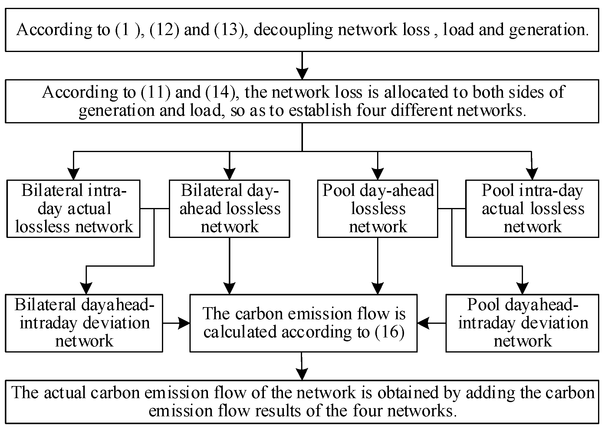
4.3. Calculation Method and Process of Actual Network Carbon Emission Flow

The actual network carbon emission flow is the sum of the day-ahead network’s carbon emission flow calculation results and the carbon emission deviation caused by the power fluctuation in the node of ‘spontaneous change’. Therefore, the carbon emission rate ${\tilde{R}}_{\mathrm{L}}$ of each node in the actual network and the carbon emission flow ${\tilde{R}}_{\mathrm{branch}}$ of each branch are as follows:

$$\left\{\begin{array}{l}{\tilde{R}}_{\mathrm{L}}=R_{\mathrm{L}}+\Delta {{\mathit{R}}^{\prime }}_{\mathrm{L}}^{\mathrm{BT}}+\Delta {{\mathit{R}}^{\prime }}_{\mathrm{L}}^{\mathrm{PT}}\\ {\tilde{\mathit{R}}}_{\mathrm{branch}}=R_{\mathrm{branch}}+\Delta {{\mathit{R}}^{\prime }}_{\mathrm{branch}}^{\mathrm{BT}}+\Delta {{\mathit{R}}^{\prime }}_{\mathrm{branch}}^{\mathrm{PT}}\end{array}\right.$$

(23)

The improved carbon emission flow solution process considering the EV charging fluctuation and hybrid power transaction is as follows:

(1)

Based on the day-ahead network and the intra-day network, the network loss is decoupled from the power generation according to (10), (12), and (13);

(2)

According to (11) and (14), the network loss is allocated to both sides of the power generation as well as consumption to establish the day-ahead lossless BT network, the day-ahead lossless PT network, the intra-day actual lossless BT network, and the intra-day actual lossless PT network;

(3)

Calculate the carbon emission flow of the day-ahead lossless network of the two transaction modes formed in step (2) according to (16)–(19) and combine them to obtain the carbon emission flow of the day-ahead network;

(4)

Using the deviation distribution method described in Section 4.2, using the four lossless networks obtained in step (2), the day-ahead-intraday lossless BT deviation network and the day-ahead-intraday lossless PT deviation network are calculated according to (20);

(5)

Find the nodes of ‘spontaneous change’ in the deviation network, calculate the carbon emission flow of the day-ahead-intraday lossless network of the two transaction modes formed in step (4) according to (16)–(19), and merge them to obtain the carbon emission of the day-ahead-intraday lossless network;

(6)

The carbon emission flow calculation results in step (3) and step (5) being added to obtain the improved power system carbon emission flow considering both EV charging fluctuation and different transaction modes.

The flow chart is shown in Figure 2.

5. Case Study

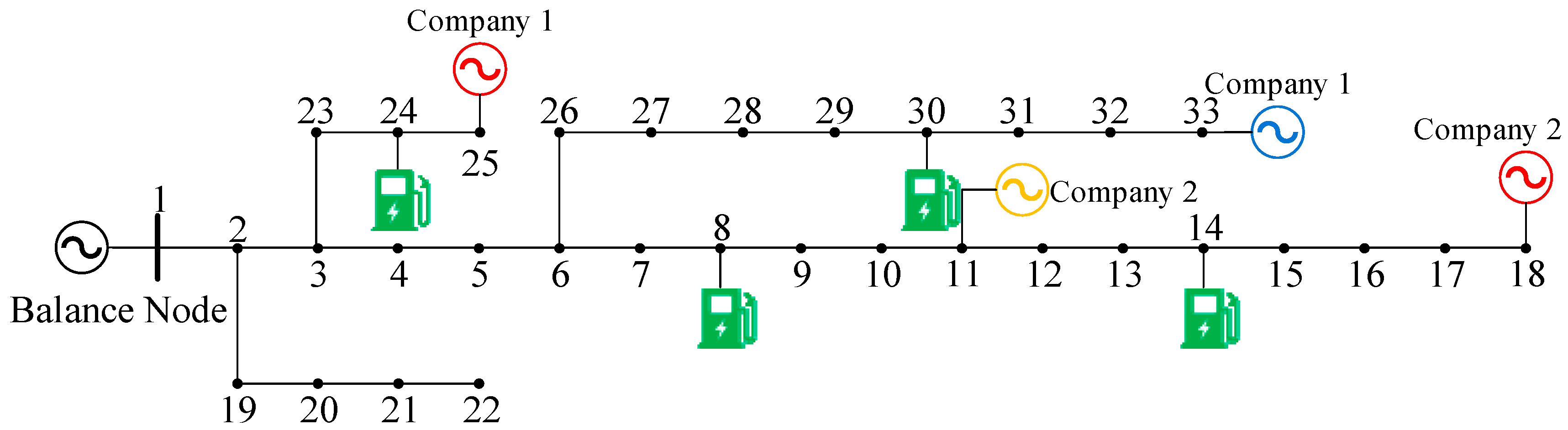
5.1. Day-Ahead Carbon Emission Flow of the IEEE-33 System

The IEEE 33 system shown in Figure 3 is used to verify the proposed method.

In Figure 3, the generator nodes have no load; node 1 is a balance node, a thermal power plant with a carbon capture device. Nodes 11, 18, 25, and 33 are generator nodes, which are photovoltaic, thermal, and hydropower plants. Among them, nodes 11, 18, 24, and 33 belong to two different power generation companies and the planned output is 340 kW, 250 kW, 320 kW, and 400 kW, respectively. Nodes 8, 14, 24, and 30 are EV charging stations participating in BT and PT modes. The power supply under the agreed BT is shown in

Table 1. The power of BT of each node.

Transaction Number	Load Node	Generator Node	Power of BT (kW)
T1	8	11	150
T2	14	18	100
T3	24	25	300
T4	30	33	160

.

To study the carbon emission changes of generators caused by EV charging, this paper assumes that other nodes only participate in the PT except for the nodes where the EV charging station is located. According to the network loss allocation method described in Section 3.2, the day-ahead lossless network after network loss allocation can be obtained, as shown in

Table 2. Parameters of the day-ahead lossless network.

Node Number	Active Power Output (kW)	Node Number	Charging Demand (kW)
1	1823.67	8	204.85
11	336.16	14	120.25
12	249.66	24	421.44
25	319.14	30	205.17
33	395.24	-	-

.

The above lossless network is divided into four BT networks and one PT network according to the transaction mode. Set E_G = [300 0 875 875 0] (tCO₂/kWh); according to the results of the improved carbon emission flow calculation model and compared with the results of the traditional carbon emission flow calculation method, the carbon emission flow rate of the node where the EV charging station is located is shown in

Table 3. Comparison of calculation results of the day-ahead network.

Node Number	Method of This Paper (tCO2/h)	Method of Tradition (tCO2/h)
8	0.01	0.05
14	0.09	0.06
24	0.33	0.31
30	0.01	0.05
others	0.60	0.57
total	1.04	1.04

.

It can be seen from the above table that compared with the traditional carbon emission flow calculation method the carbon emission of the whole network has stayed the same. However, the following characteristics are presented on the load side:

(1)

For the carbon emission flow rates borne by nodes 14 and 24 of the BT agreement with the thermal power plant, the traditional carbon emission flow calculation method results are 0.06 tCO₂/h and 0.31 tCO₂/h, respectively. In comparison, the results calculated by the improved carbon emission flow method in this paper are 0.09 tCO₂/h and 0.33 tCO₂/h, 50.00% and 6.44% higher than those. Among them, because nodes 24 and 25 are adjacent, the power injected into the grid by node 25 flows through node 24 whether the power consumption agreement is signed, so the carbon emission flow rate of node 24 obtained by the two methods changes less;

(2)

For the carbon emission flow rate of node 8, which signed a BT agreement with a photovoltaic power plant, and node 30, which signed a BT agreement with a hydropower plant, the results obtained by using the traditional carbon emission flow calculation method are 0.05 tCO₂/h. In comparison, the results calculated using the improved carbon emission flow calculation method in this paper are 0.01 tCO₂/h, which is 80% lower;

(3)

The rest of the nodes only participate in the PT. Since nodes 14 and 24 bear part of the carbon emission, the results of the day-ahead carbon emission flow calculation method proposed in this paper are lower than those of the traditional carbon emission flow calculation method.

The day-ahead carbon emission flow calculation method proposed in this paper aligns with the expectation of purchasing more low-carbon electricity and distributing less carbon emissions. Therefore, the day-ahead carbon emission flow calculation method proposed in this paper can encourage EV charging stations to sign BT agreements with clean energy power plants and can positively guide EV users to charge charging stations that sign BT agreements with clean energy power plants, thereby promoting the consumption of clean energy power.

5.2. The Actual Carbon Emission Flow of the IEEE-33 System

In the intra-day operation stage, the actual output of photovoltaic power generation node 11 is 200 kW, the actual charging demand of load node 8 is 100 kW higher than the predicted value, and the actual charging demand of load node 14 is 15 kW lower than the predicted value. The actual load demand of the remaining nodes is consistent with the expected value.

In the BT network, nodes 8, 11, and 14 are ‘spontaneous change’ nodes. Due to the fact that the charging demand of node 8 increases and the output of node 11 decreases, it is impossible to match the agreement power of BT. It is necessary to match the BT agreement power with node 18 of the same power generation company so the actual output of node 18 increases to 350 kW. After converting the actual intra-day network into a lossless network, it is decomposed according to different transaction modes. The charging demand and unit output are shown in

Table 4. Load and unit output of the day-ahead-intraday deviation network (kW).

Node Number	T1		PT
	Charging Demand	Active Power Output	Charging Demand	Active Power Output
1	-	-	-	134.50
8	103.35	-	-	-
11	-	(103.35)	-	−244.06
14	-	-	−11.64	-
18	-	103.35	-	98.83
24	-	-	-	-
25	-	-	-	−0.17
30	-	-	-	-
33	-	-	-	−0.74

.

By calculating the carbon emission flow under each transaction mode in Table 4, the carbon emission flow changes caused by the charging fluctuation in EVs and the prediction error of generator output can be obtained, as shown in

Table 5. Carbon emission flow of day-ahead-intraday deviation network.

Node Number	T1 (tCO2/h)	PT (tCO2/h)	Total (tCO2/h)
8	0.09	-	0.09
14	-	−0.01	−0.01

.

From the carbon flow rate of each node of the day-ahead network and the day-ahead-intraday deviation network obtained from Table 3 and Table 5, the carbon emission flow of the actual network can be obtained, as shown in

Table 6. Comparison of calculation results of the actual network in intra-day.

Node Number	Method of This Paper (tCO2/h)	Method of Tradition (tCO2/h)
8	0.01	0.09
11	0.10	0
14	0.18	0.09
24	0.31	0.31
30	0.01	0.05

.

From Table 6, for generator node 11, due to the inability to match the BT agreement power within the day, it is generated by generator node 18 of the same power generation company. In contrast, node 18 is the thermal power generator and the carbon emission caused by it should be shared by node 11. Therefore, the carbon flow rate of node 11 calculated by the proposed method is 0.10 tCO₂/h, which is more realistic.

6. Conclusions

This paper proposes a more reasonably improved carbon emission flow model considering EV charging fluctuation and hybrid power transactions; the model is simulated and verified by the IEEE-33 system. The following conclusions are drawn:

(1)

This paper decouples different transaction modes in the day-ahead network by establishing a lossless network. Based on the nonlinear carbon emission flow calculation relationship, carbon emission responsibility can be more accurately divided into different transaction types. Under the premise of making the division of carbon emissions more equitable, this calculation method can also encourage EV charging stations to sign BT agreements with clean energy power plants and guide EV users to charge their charging stations, thus promoting the consumption of clean energy power;

(2)

In the intra-day network, this paper finds the ‘active change’ node by comparing the charging demand and unit output of the day-ahead network and divides the node of ‘spontaneous change’ into different transaction types according to the characteristics of different transaction modes; it finally establishes the day-ahead-intraday deviation network. Through the day-ahead-day deviation network, the reasons for the changes in carbon emissions in the network are found and the resulting changes in carbon emissions are attributed to the node of ‘spontaneous change’. This calculation method does not simply attribute the carbon emission of the power generation side to the thermal power generating unit, which can enable EV users to personally experience the change in carbon emissions caused by the change in their electricity consumption behavior to the power grid. It does so in order that the carbon emission calculation of the unit is fairer, which lays a theoretical foundation for the setting of time-of-use electricity price based on carbon emission.

In summary, with the implementation of energy conservation and the popularization of the low-carbon concept, we must pay attention to the reasonable attribution of carbon emissions. The method proposed in this paper can provide EV users with specific components of carbon emission in different transaction modes and promote clean energy consumption. It can also make EV users feel the change in carbon emission, improve the output prediction accuracy of each generator set, and promote the update of new energy technologies.

References

1. He, J.K. New mechanism and influence of “Paris Agreement”. World Environ. 2016, 10, 16–18. [Google Scholar]
2. Cui, Y.; Zeng, P.; Hui, X.; Li, H.; Zhao, J. Low-carbon economic dispatch considering the integrated flexible operation mode of carbon capture power plant. Power Syst. Technol. 2021, 45, 1877–1885. [Google Scholar]
3. Han, X.; Li, T.; Zhang, D.; Zhou, X. New issues and key technologies of new power system planning under double carbon goals. High Volt. Eng. 2021, 47, 3036–3046. [Google Scholar]
4. Cui, Y.; Zeng, P.; Wang, Z.; Wang, M.; Zhang, J.; Zhao, Y. Low-carbon economic dispatch of electricity-gas-heat integrated energy system with carbon capture equipment considering price-based demand response. Power Syst. Technol. 2021, 45, 447–459. [Google Scholar]
5. Shao, S.N.; Rahmans, P. Challenges of PHEV penetration to the residential distribution network. In Proceedings of the IEEE Power & Energy Society General Meeting, Calgary, AB, Canada, 26–30 July 2009; pp. 2522–2529. [Google Scholar]
6. Wang, X.; Zhao, J.; Wang, K.; Yao, J.; Yang, S.; Feng, S. Multi-Objective Bi-Level Electric Vehicle Charging Optimization Considering User Satisfaction Degree and Distribution Grid Security. Power Syst. Technol. 2017, 41, 2165–2172. [Google Scholar]
7. Jiang, Z.; Xiang, Y.; Liu, J. Charging Load Modeling Integrated with Electric Vehicle Whole Trajectory Space and Its Impact on Distribution Network Reliability. Power Syst. Technol. 2019, 43, 3789–3800. [Google Scholar]
8. Li, M. Research on Evaluation of Electric Vehicle Acceptance Capacity in Local Distribution Network; Jiaotong University: Beijing, China, 2018. [Google Scholar]
9. Zhang, L.; Xu, Y.; Hu, H.; Zhang, Z. Evaluation Indices and Method for Electric Vehicles Impact on Power Grid. Electr. Power Constr. 2013, 34, 47–51. [Google Scholar]
10. Chen, L.; Sun, T.; Zhou, Y.; Zhou, E.; Fang, C.; Feng, D. Method of carbon obligation allocation between generation side and demand side in power system. Autom. Electr. Power Syst. 2018, 42, 106–111. [Google Scholar]
11. Wang, C.; Lu, Z.; Qiao, Y. A consideration of the wind power benefits in day-ahead scheduling of wind-coal intensive power systems. IEEE Trans. Power Syst. 2013, 28, 236–245. [Google Scholar] [CrossRef]
12. Chattopadhyay, D. Modeling greenhouse gas reduction from the Australian electricity sector. IEEE Trans. Power Syst. 2010, 25, 729–740. [Google Scholar] [CrossRef]
13. Gil, H.; Joos, G. Generalized estimation of average displaced emissions by wind generation. IEEE Trans. Power Syst. 2007, 22, 1035–1043. [Google Scholar] [CrossRef]
14. Lenzen, M.; Munksgaard, J. Energy and CO2 life-cycle analyses of wind turbines-review and applications. Renew. Energy 2002, 26, 339–362. [Google Scholar] [CrossRef]
15. Chen, H.; Mao, W.; Zhang, R.; Yu, W. Low-carbon optimal scheduling of a power system source-load considering coordination based on carbon emission flow theory. Power Syst. Prot. Control. 2021, 49, 1–11. [Google Scholar]
16. Kang, C.; Zhou, T.; Chen, Q.; Wang, J.; Sun, Y.; Xia, Q.; Yan, H. Carbon emission flow from generation to demand: A network-based model. IEEE Trans. Smart Grid 2015, 6, 2386–2394. [Google Scholar] [CrossRef]
17. Zhou, T.; Kang, C.; Xu, Q.; Chen, Q. Preliminary theoretical investigation on power system carbon emission flow. Autom. Electr. Power Syst. 2012, 36, 38–43. [Google Scholar]
18. Bialek, J. Tracing the flow of electricity. IEEE Proc. Gener. Transm. Distrib. 1996, 143, 313–320. [Google Scholar] [CrossRef]
19. Kirschen, D.; Allan, R.; Strbac, G. Contributions of individual generators to loads and flows. IEEE Trans. Power Syst. 1997, 12, 52–60. [Google Scholar] [CrossRef]
20. Abdelkader, S.M. Allocating transmission loss to loads and generators through complex power flow tracing. IET Gener. Transm. Distrib. 2007, 1, 584–595. [Google Scholar] [CrossRef]
21. Cheng, Y.; Zhang, N.; Wang, Y.; Yang, J.; Kang, C.; Xia, Q. Modeling carbon emission flow in multiple energy systems. IEEE Trans. Smart Grid 2019, 10, 3562–3574. [Google Scholar] [CrossRef]
22. Gong, Y.; Jiang, C.; Li, M.; Wang, X.; Li, L. Carbon emission calculation on power consumer side based on complex power flow tracing. Autom. Electr. Power Syst. 2014, 38, 113–117. [Google Scholar]
23. Zhou, T.; Kang, C.; Xu, Q.; Chen, Q.; Xin, J.; Wu, Y. Analysis on distribution characteristics and mechanisms of carbon emission flow in electric power network. Autom. Electr. Power Syst. 2012, 36, 39–44. [Google Scholar]
24. Yuan, S.; Ma, R. A research on the allocation model of carbon emission in power system based on carbon emission flow theory. Mod. Electr. Power 2014, 31, 70–75. [Google Scholar]
25. Zhou, Q.; Feng, D.; Xu, C.; Feng, C.; Sun, T.; Ding, T. Methods for allocating carbon obligation in demand side: A comparative study. Autom. Electr. Power Syst. 2015, 39, 153–159. [Google Scholar]
26. Kang, C.; Cheng, Y.; Sun, Y.; Zhang, N.; Meng, J.; Yan, H. Recursive calculation method of carbon emission flow in power systems. Autom. Electr. Power Syst. 2017, 41, 10–16. [Google Scholar]
27. Melgar-Dominguez, O.D.; Pourakbari-Kasmaei, M.; Lehtonen, M.; Mantovani, J.R.S. An economic-environmental asset planning in electric distribution networks considering carbon emission trading and demand response. Electr. Power Syst. Res. 2020, 181, 106202. [Google Scholar] [CrossRef]
28. Chen, D.; Xian, W.J.; Wu, T.; Guo, R.P. Allocation of Carbon Emission Flow in Hybrid Electricity Market. Power Syst. Technol. 2016, 40, 6. [Google Scholar]
29. Wang, C.; Chen, Y.; Wen, F.; Tao, Y.; Chi, C.; Jiang, X. Some Problems and Improvement of Carbon Emission Flow Theory in Power Systems. Power Syst. Technol. 2022, 46, 1683–1693. [Google Scholar]
Figure 1. Node splitting model. Where P G i and P L j are the total injection power of generator node i and the outflow power of load node j, respectively; P G i BT and P G i PT are the power injected by generator node i in BT and PT mode, respectively; and P L j BT and P L j PT are the outflow power of load node j in BT and PT modes, respectively.
Energies 16 06835 g001
Figure 2. Calculation flow chart.
Energies 16 06835 g002
Figure 3. Illustration of the IEEE-33 system.
Energies 16 06835 g003