Article

Mathematical Modeling of Alkaline Direct Glycerol Fuel Cells

by
Alessandra Pezzini
1,
Ubiranilson João de Castro
1,
Deborah S. B. L. de Oliveira
2,
Germano Tremiliosi-Filho
3 and
Ruy de Sousa Júnior
1,*
1
Graduate Program in Chemical Engineering, Federal University of São Carlos, Rod. Washington Luís, km 235, São Carlos 13565-905, SP, Brazil
2
Faculty of Engineering and Physical Sciences, University of Leeds, Leeds LS2 9JT, UK
3
São Carlos Institute of Chemistry, University of São Paulo, Avenida Trabalhador São-carlense, 400, São Carlos 13566-590, SP, Brazil
*
Author to whom correspondence should be addressed.
Energies 2023, 16(19), 6762; https://doi.org/10.3390/en16196762
Submission received: 1 September 2023 / Revised: 17 September 2023 / Accepted: 19 September 2023 / Published: 22 September 2023
(This article belongs to the Section A5: Hydrogen Energy)

Abstract

:
Mathematical modeling and computer simulation are tools of great importance for the development of fuel cells. Thus, the objective of this work is to carry out the kinetic modeling of glycerol oxidation in a DGFC (direct glycerol fuel cell), considering two different approaches: (1) realistic phenomenological models for the partial oxidation of glycerol in Pt/C, considering its adsorbed intermediates; (2) models of artificial neural networks (ANN—artificial neural networks) for oxidation mainly of PtAg/C and PtAg/MnOx/C. The models were fitted to experimental data already available for validation and determination of their parameters, both using Matlab software, v. R2018a (MathWorks, Natick, MA, USA). Results for the phenomenological models developed showed excellent fits for the polarization curve, with an RMSE (root mean squared error) value on the order of 0.352 to 0.404 mA/cm2, in addition to coverage fractions consistent with the literature for the adsorbed species. The kinetic parameters with the greatest influence on the response of the models were those associated with the consumption of glyceric acid and the formation of tartronic acid and with the dissociative adsorption of water and the formation of Pt-Oads active sites. Regarding the neural models, excellent prediction fits were obtained for all of them, with RMSE values on the order of 0.008 to 0.014 mA/cm2, indicating the possibility of representing the functional interdependence between input variables and the density cell current for cases where it would be too complex to do so via mechanistic modeling (i.e., for PtAg/C and PtAg/MnOx/C oxidation).

1. Introduction

Glycerol is the main co-product of biodiesel manufacture, with its output exceeding the traditional market demand (largely due to the continuing increase in biodiesel production). Therefore, it is necessary to find new applications for this polyol. The oxidation of glycerol in fuel cells is operationally feasible and can enable the production of energy and chemicals that are of interest and difficult to obtain [1,2,3].
Activation of the oxidation reactions of alcohols, such as glycerol, is facilitated in an alkaline medium [4,5,6]. It is difficult to fully oxidize glycerol in both acidic and alkaline media due to the difficulty in breaking the C-C bonds, leading to parallel partial oxidation reactions [1]. Oxidation of the primary hydroxyl of glycerol can result in the formation of glyceraldehyde, glyceric acid, glycolic acid, oxalic acid, and tartronic acid, among other compounds, while oxidation of the secondary hydroxyl leads to the formation of dihydroxyacetone and hydroxypyruvic acid [7,8]. It is known from many experimental studies reported in the literature that optimization of the operating conditions (such as the type and properties of the catalyst) can enable the selectivity of the reaction to be directed towards oxidation of either the primary or the secondary hydroxyl [7,8,9,10,11]. According to Behr et al. [7], Pt electrodes are more selective towards the oxidation of the primary hydroxyl of glycerol, leading to the formation of glyceraldehyde and other oxidized compounds, as observed in several studies [1,3,12]. The addition of bismuth (Bi) to the catalyst composition favors the production of dihydroxyacetone, with increased selectivity towards oxidation of the secondary hydroxyl of glycerol [12,13,14,15,16,17]. This is because Bi acts to block the active sites of the platinum catalyst that would oxidize the primary hydroxyl [14].
Kwon et al. [3] outlined a reaction mechanism for the oxidation of glycerol in alkaline media using Au and Pt electrodes. In the pathway of primary alcohol oxidation, glycerol is first oxidized in a two-electron transfer step to glyceraldehyde, which is subsequently oxidized to glyceric acid. In the case of the gold electrode, glyceric acid is apparently directly produced from glycerol via glyceraldehyde. As a next transfer step, glyceric acid is further oxidized via cleavage of a C-C bond into glycolic acid and formic acid on both electrodes. In particular, on the platinum electrode at potentials close to 0.9 V, this process becomes deactivated because Pt forms an inhibiting surface oxide. The Au electrode has a much higher conversion activity of glyceric acid to glycolic acid and formic acid than does the Pt electrode. In addition, glyceric acid and glycolic acid are further oxidized on the platinum electrode to tartronic acid and oxalic acid. In the pathway of secondary alcohol oxidation, dihydroxyacetone might be produced [3]. The main product is glyceric acid, with glyceraldehyde as an intermediate, while low selectivity has been observed towards dihydroxyacetone. Both the activity and the products formed are highly dependent on the catalyst and pH, although the general pathways of the mechanism does not change. The production of dihydroxyacetone is minimal, with the platinum electrode showing preferential oxidation of the primary hydroxyl of glycerol.
One feasible way to use glycerol is in solid alkaline membrane fuel cells (SAMFCs), which are a hybridization of solid polymer electrolyte fuel cells (SPEFCs) with alkaline fuel cells (AFCs) [18]. An alkaline direct glycerol fuel cell (DGFC) with a polymeric membrane and fed with glycerol can be considered an SAMFC. Nonetheless, it is acknowledged that the electrical performance of DGFCs still requires many improvements, mainly related to the activity of the catalysts and the cell’s operational parameters.
Mathematical modeling is a very important tool for facilitating the development of new designs of these devices, reducing the amount of experimental work required [19]. Studies have shown that the glycerol oxidation reaction in a DGFC is highly complex due to the many adsorbed intermediates formed during the partial oxidation of glycerol [1,3]. The mechanistic modeling approach is suitable to be applied to fuel cells, being described by expressions representing electrochemical and transport phenomena [20,21]. Additionally, the use of artificial neural networks (ANNs) enables representation of the functional dependence between cell potential and current density in cases where it would be currently unfeasible to develop complete mechanistic models capable of accurately describing all the mechanisms involved. In particular, bimetallic electrodes for glycerol oxidation present greater mechanistic complexity compared to monometallic electrodes. In those cases, where the mechanisms are even more complex, ANNs can provide predictions of the functional relationships among the variables involved. This way, modelling based on mechanisms and ANNs are complementary tools.
Therefore, modeling of these systems can also take advantage of empirical models, including artificial neural networks that are able to learn the behavior of the system from experimental data [22]. The simulation and modeling of direct ethanol fuel cells (DEFCs) is well documented in the literature, notably the pioneering work by Sousa Jr. et al. [23], who developed a phenomenological model for DEFC simulation. Maia and Sousa Jr. [24] studied DEFCs by adopting a mechanistic approach and the use of CFD, while more recent works by de Oliveira et al. [25] and Oliveira et al. [26] employed mechanistic and neuro-fuzzy approaches, respectively, for simulation of a DEFC. For simulation of the oxidation of glycerol in DGFCs, the literature lacks studies addressing the full complexity of this reaction. The simulation work by Han et al. [27] only considered the formation of tartronic acid, while experimental studies [1,3] reported up to six products formed in the reaction. Another gap in the literature concerning DGFCS simulation is the lack of more extensive statistical studies of the model kinetic parameters, while no work has considered any type of computational intelligence applied to glycerol oxidation in fuel cells.
In this work, mathematical modeling of direct glycerol fuel cells was performed using phenomenological equations and artificial neural networks, together with statistical evaluation and determination of mechanistic model parameter sensitivity. For this, based on the data from the research presented in Garcia et al. [28] and the partial oxidation mechanism on Pt/C electrodes proposed by Kwon et al. [3], the kinetic parameters of a phenomenological model were fitted using the fmincon function of Matlab software. Additionally, a statistical study of the parameter fits was performed and parameter sensitivity was assessed. Finally, a multilayer perceptron (MLP) neural network model was obtained, fitted to the data from Garcia et al. [28], applicable to oxidation on PtAg/C and PtAg/MnOx/C electrodes.
In the case of the phenomenological model, there are some important contributions to the state of the art of DGFCs, namely provision of a more complex and comprehensive model that includes consideration of different intermediates of the partial oxidation of glycerol in a fuel cell, which can be used to obtain more simplified models. There is the need for such a general model with a solid theoretical background which can accurately describe the reaction behavior; statistical study of the model kinetic parameters provides essential information concerning the specific parameters that significantly influence the behavior of the polarization curve and the distribution of the many adsorbed intermediates produced in the reaction. These parameters can be precisely determined via the parameter fitting method (since they present lower standard deviation values); finally, elucidation of possible variations in the distribution profiles of the adsorbed intermediates can show the interdependence between the model parameters and the degree of coating of the catalyst. This can enable evaluation of possible changes in the amount of a particular product actually obtained. The availability of a comprehensive phenomenological model with well-defined kinetic parameters, supported by statistical evaluation, enables robust description of the experimental behavior and possible reaction mechanisms.
Concerning the neural network approach, there are still no studies in the literature that have addressed this type of artificial intelligence applied to DGFCs, so the present work contributes to filling this gap, demonstrating the importance of a black box model applied to complex systems. The use of both types of modeling also enables assessment of the predictive ability of each approach.
In what follows, sections are organized according to the structure of topics presented. Methods (Section 2) describes a realistic phenomenological model (Section 2.1), including a complete phenomenological model at 60 °C (Section 2.1.1); additional mechanistic models developed (Section 2.1.2), which encompass the simplified models and a phenomenological model at 90 °C; and artificial neural networks (Section 2.2), including training, validation, and testing of the neural network (Section 2.2.1), neural network performance assessment (Section 2.2.2), and a neural network for PtAg/C and PtAg/MnOx/C electrodes at 60 °C and 90 °C (Section 2.2.3). Results and discussion (Section 3) describes phenomenological models (Section 3.1), including a phenomenological model at 60 °C (Section 3.1.1), simplified models 1 and 2 (Section 3.1.2), a comparison between the full model at 60 °C and simplified models 1 and 2 (Section 3.1.3), a phenomenological model at 90 °C (Section 3.1.4), additional validation of PMs at 60 °C and 90 °C (Section 3.1.5), and a neural network developed for PtAg/C and PtAg/MnOx/C electrodes at 60 °C and 90 °C (Section 3.2); and the pros and cons of the developed models (Section 3.3). After our conclusions (Section 4), Appendix A contains the equations for the formation of the corresponding salts (glycerate, tartronate, glycolate, formate, oxalate) in alkaline media.

2. Materials and Methods

2.1. Realistic Phenomenological Model

The modeling of real systems allows for analysis of the process and greater understanding of its intrinsic mechanisms. Model fitting is performed by optimizing parameter values, where the main objective is to approximate the model result ŷ(i) to the measured process output variable y(i) by fitting the n parameters of the model contained in the vector θ [29]. The main procedure for aligning a model to experimental values, including kinetic data, employs the least squares regression method [29,30] to obtain values for the θ parameters of the model that minimize the value of the objective function I(θ). This objective function is related to the residual (e); the smaller this residual is, the closer the process and model outputs [29].
The function to be minimized is subject to equality and/or inequality constraints, which are equations that constrain the search area for the local optimal value, and may be linear or nonlinear. Other factors defining the value of this optimal point are the initial estimates and the lower and upper limits of each parameter.
The Hessian matrix (H), which is a square matrix containing information for the second-order derivative of the objective function in relation to the parameters, is of great importance for the precision of the parameters to be fitted. For linear models, this matrix is obtained according to Equation (1).
H _ = 2 I θ _ θ _ 2 = X _ T X _
where X is the derivative of the error e with respect to the parameters θ, representing the sensitivity with respect to them.
The most popular method of solving constrained nonlinear optimization problems is sequential quadratic programming (SQP) [31]. The parameters of a model can be estimated with varying precision, so it is essential to calculate their statistical aspects, such as variance and standard deviation. The variance of the parameters can be obtained using the variance–covariance matrix (CVR) [29].
After making the necessary adjustments and considering the noise, the covariance matrix can be approximated using Equation (2), obtaining the correlation of this matrix with the Hessian matrix and the noise variance [29]. The matrix parameters are assumed not to be correlated with each other, so the absolute value of the diagonal of the variance–covariance matrix is the variance itself (CVR (i, i)), with the other values corresponding to the covariance between two parameters. The standard error (SE) is given by the square root of the variance (Equation (3)), while the standard deviation (SD), shown in Equation (4), considers a two-tailed confidence interval of 95% [32].
CVR θ ^ _ σ 2 X _ T X _ 1 σ 2 H _ 1
SE = CVR ( i , i )
SD = t value SE
SD and SE are vectors with size np (where np is the number of parameters), and tvalue is the value of the Student’s t-statistic.
Efficient models are obtained when the regressors have higher values and the noise variance values are lower. The parameter sensitivity can be estimated via the partial derivative of the error in relation to a particular parameter. Greater sensitivity of the error in relation to the parameters is associated with a smaller variance value [29].
Equation (2) was adjusted for noise, so an alternative is required for cases where the data noise is unknown. Hence, the variance can be estimated from the residuals, as shown in Equation (5), where the denominator represents the number of degrees of freedom for problems with constraints (c), considering the number of parameters (np) and sample size (N), with the term σ2 representing the noise variance [29].
σ 2 = e _ T e _ N np + c = SSE N np + c
Kinetic modeling of a direct glycerol fuel cell was performed according to the phenomenological approach using fundamental electrochemical kinetic equations, as well as with a black box model using artificial neural networks. In both approaches, the modeling was based on the experimental data obtained by Garcia et al. [28]. The fuel cell used was the alkaline type with a polybenzimidazole (PBI) type anion transport membrane, doped with KOH (potassium hydroxide). The anode was fed 1 M glycerol + 4 M KOH at a rate of 1 mL/min, and the cathode was fed O2 (oxygen) at 30 mL/min. The catalyst types used were Pt/C, PtAg/C, and PtAg/MnOx/C. A schematic illustration of an SAMFC similar to the one used is shown in Figure 1.
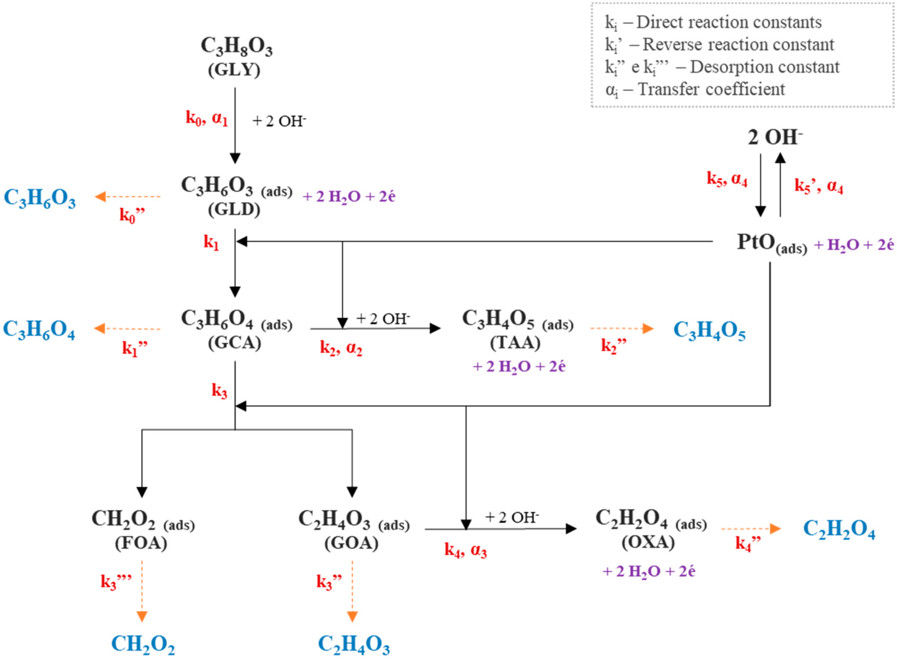
The phenomenological model was mainly based on the mechanism proposed by Kwon et al. [3], supported by Zhou et al. [10], which does not consider complete oxidation to CO2 but involves partial oxidation reactions with adsorbed intermediates. The reaction pathway for oxidation of the secondary hydroxyl of glycerol was neglected, since when a Pt electrode is used in an alkaline medium, oxidation to glyceraldehyde and other products is favored, as widely reported in the literature.
Realistic phenomenological modeling was only performed using a Pt/C electrode, since understanding and describing the other composite electrodes would be considerably more complex, requiring a very high number of parameters (overparameterization). For these cases, the neural network approach was used as described in Section 2.2. The model considered the formation of glyceraldehyde (GLD), glyceric acid (GCA), glycolic acid (GOA), tartronic acid (TAA), formic acid (FOA), and oxalic acid (OXA). The kinetic steps considered in the phenomenological model are given by Equations (6)–(17).
C 3 H 8 O 3 + 2 OH C 3 H 6 O 3 ads + 2 H 2 O + 2 e k 0
C 3 H 6 O 3 ads C 3 H 6 O 3 k 0
C 3 H 6 O 3 ads + PtO ads C 3 H 6 O 4 ads k 1
C 3 H 6 O 4 ads C 3 H 6 O 4 k 1
C 3 H 6 O 4 ads + PtO ads + 2 OH C 3 H 4 O 5 ads + 2 H 2 O + 2 e k 2
C 3 H 4 O 5 ads C 3 H 4 O 5 k 2
C 3 H 6 O 4 ads + PtO ads C 2 H 4 O 3 ads + C H 2 O 2 ads k 3
C 2 H 4 O 3 ads C 2 H 4 O 3 k 3
C H 2 O 2 ads C H 2 O 2 k 3
C 2 H 4 O 3 ads + PtO ads + 2 OH C 2 H 2 O 4 ads + 2 H 2 O + 2 e k 4
C 2 H 2 O 4 ads C 2 H 2 O 4 k 4
2 OH PtO ads + H 2 O + 2 e k 5 ,   k 5
It is worth mentioning that in the case of an alkaline medium, in reality the salts of the aforementioned acids are produced, and the equations for this case are found in Appendix A (Equations (A1)–(A12)). However, as is demonstrated by several studies, including Kwon et al. [3], the formation of acids will be considered for modeling, since this consideration does not invalidate anything that is related to the model, as it can be observed that the chemical equations referring to the formation of salts (Equations (A1)–(A12), Appendix A) are similar to those that consider the formation of acids (Equations (6)–(17)), maintaining the same release of electrons in both conditions. Figure 2 presents a scheme that encompasses all reactions from Equations (6)–(17), showing the mechanism that was then considered for the working model.

2.1.1. Complete Phenomenological Model at 60 °C

The main mechanistic model developed was for the oxidation of glycerol in an alkaline DGFC with a Pt/C electrode at a working temperature of 60 °C. The main assumptions are presented as follows.

Calculation of Anodic Overpotential

The experimental data of Garcia et al. [28] were in the form of cell potential (Vcel) versus current density (i). However, the phenomenological model was based on anodic overpotential (ηA), so it was necessary to obtain this value using Equation (18), which considers the real measured cell potential (Vcel); the real measured current density (i); the open circuit potential (E0), which was adjusted to the ideal model; the concentration overpotential (ηconc), calculated using Equation (19), whose limiting current was obtained based on extrapolation of the experimental data (and provided a good description of the behavior of the curve); the membrane resistance to the ion transport (Rmem); and the cathode overpotential (ηC), calculated using Equation (20) [23].
V cel = E 0 η A η C R m i η Conc
η Conc = RT F ln i L i L i
η C = RT α C F ln i C i 0 C O 2 , ref C O 2
Table 1 shows the values used for the constants in Equations (18)–(20), as well as for calculation of the model constraint and current density equations.

Constraint Equations and Current Density Calculation

The model constraint equations were based on the steady-state mass balance of all the adsorbed intermediates coating the electrode (Equations (21)–(27)), totaling seven equality constraint equations. These equations were based on partial reaction Equations (6)–(17), while the terms containing electron exchange (oxidation or reduction) were based on the Butler–Volmer equation. Terms for desorption of the intermediates adsorbed on the catalyst were also included.
Γ d θ GLD dt = 0 = k 0 C GLY 1 θ e α 1 F RT η k 0 θ GLD k 1 θ GLD θ PtO
Γ d θ GCA dt = 0 = k 1 θ GLD θ PtO k 1 θ GCA k 2 θ GCA θ PtO e α 2 F RT η k 3 θ GCA θ PtO
Γ d θ TAA dt = 0 = k 2 θ GCA θ PtO e α 2 F RT η k 2 θ TAA
Γ d θ GOA dt = 0 = k 3 θ GCA θ PtO k 3 θ GOA k 4 θ GOA θ PtO e α 3 F RT η
Γ d θ FOA dt = 0 = k 3 θ GCA θ PtO k 3 θ FOA
Γ d θ OXA dt = 0 = k 4 θ GOA θ PtO e α 3 F RT η k 4 θ OXA
Γ d θ PtO dt = 0 = k 1 θ GLD θ PtO k 2 θ GCA θ PtO e α 2 F RT η k 3 θ GCA θ PtO k 4 θ GOA θ PtO e α 3 F RT η + k 5 1 θ e α 4 F RT η k 5 θ PtO e ( 2 α 4 ) F RT η
The above equations are written as a function of the thirteen reaction kinetic constants (k’s), the fractions of the adsorbed intermediates (θi), and four transfer coefficients (αi) that take into account the number of electrons exchanged in the reaction (being, in practice, n times the transfer coefficient). The kinetic constants are in units of mol/(m2·s), with the exception of k0 (units of m/s), and the transfer coefficients and coverage fractions are dimensionless. The inequality constraint is designated by ∑θi ≤ 1, since at each experimental data point, the sum of all the adsorbed species fractions cannot be greater than 1, according to the law of conservation of mass. However, this inequality constraint did not need to be implemented in the programming, since the steady-state mass balances already ensured that it was respected.
The calculated current density (ical) was obtained by summing all the terms that contained electron exchange (in Equations (21)–(27)) and multiplying by the number of electrons exchanged in the reaction and by the Faraday constant. Since all the reactions always exchanged 2 electrons, the equation for calculation of the current density (with units of A/m2) was as shown in Equation (28).
i cal = 2 F ( k 0 C GLY 1 θ e α 1 F RT η A + k 2 θ GCA θ PtO e α 2 F RT η A + k 4 θ GOA θ PtO e α 3 F RT η A + k 5 1 θ e α 4 F RT η A k 5 θ PtO e ( 2 α 4 ) F RT η A )

Nonlinear Regression with Constraints

The phenomenological model simulation employed the fmincon tool from Matlab, which finds the minimum value for a function according to a regression process. This was applied for the minimization of the sum of squared errors (SSE) between the experimental current density (iexp), obtained by Garcia et al. [28], and the calculated current density (ical), obtained using Equation (28). This function admits the presence of equality and inequality constraints. The syntax of the fmincon function is demonstrated by Equation (29).
x , SSE , Hessian = fmincon @ function , x 0 , A , b , A eq , b eq , lb ,   ub , @ nonlcon , options
The model output arguments are: x, which are the adjusted values of each parameter; SSE, the sum of squared errors at the end of optimization; and Hessian, the square matrix p×p, where p denotes the number of parameters. The algorithm inputs are: @function, which receives the function (Equation (28), from the current density calculation) to be used in the minimization of the SSE; x0, a vector that contains the initial guesses for each parameter; A, b, Aeq and beq, vectors and matrices referring to the linear inequality and equality constraints, respectively; lb and ub, which denote the values of the lower and upper limits for each parameter, respectively; @nonlcon, which receives the set of nonlinear constraints of equality (Equations (21)–(27)) and inequality (recalling that it was not necessary to implement the condition ∑θi ≤ 1 in the algorithm, since steady-state mass balances already guarantee that it is respected); and lastly, the “options” argument, which makes available certain preferences for the algorithm, such as the number of epochs and type of optimization algorithm used, which in this case was SQP (sequential quadratic programming).
The approximated covariance matrix was calculated using the Hessian matrix generated by the fmincon function, based on the second-order derivative of the Lagrangian, which was used as an approximation of XTX (Equation (1)).
The first optimization step was to fit the polarization curve to the experimental data, in other words, to fit the curve of anode overpotential (ηA) plotted against current density (i). The fit was performed and analyzed point by point, with the resulting calculated current density value being as close as possible to the experimental value. The SSE value obtained was used to calculate the RMSE (root mean squared error) and the variance of the noise of the experimental data by Equation (5). The lower and upper limits and the initial guesses of the kinetic constants and transfer coefficients were kept constant in this step. The initial guesses and lower and upper limits for the coverage fractions were based on the selectivity curve obtained by Kwon et al. [3]. For the kinetic parameters, they were obtained previously by the present research group, by trial and error, in order to satisfy the constraints and find a good fit of the polarization curve.

Statistical Study of the Parameters

After completing the regression process and adjusting the model parameters, the fmincon function generated the final SSE value, which was the sum of the squared errors between the experimental data and the calculated current density values. The smaller this value is, the closer the model response is to the experimental data. One of the outputs obtained using the fmincon function was the Hessian matrix, which was used to calculate the approximate covariance matrix (Equation (2)). Then, with this matrix and the variance of the noise, it was possible to calculate the SE and SD values using Equations (3) and (4).

Determination of the Model Parameters with Greatest Influence

For the initial fitting, the adjustable parameters considered were the fractions of all the adsorbed intermediates (minus the fraction of six intermediates that were properly fixed as being zero at ηA = 0 V), the kinetic constants, and the transfer coefficients. After the polarization curve was fitted, the coverage fractions varied within a narrow search range and the kinetic parameters presented high SD values, as expected for a model with many parameters. Therefore, the first step in identifying the most sensitive model parameters was to maintain the coverage fraction values constant in the subsequent adjustments, with only the kinetic constants and the transfer coefficients as adjustable parameters. It should be noted that the SD and SE values referred only to the error related to the parameter sensitivity and noise variance.
Determination of the most sensitive parameters used the subset selection method in backward elimination mode with stepwise selection. Accordingly, after an initial fitting with all the parameters, the parameter to be fixed was chosen based on a statistical value (stepwise selection), in this case the relative SD value (the SD value divided by the adjusted value of the parameter), and the parameters were fixed one at a time, until only the most sensitive parameter remained (backward elimination) [29].

Parameter Sensitivity (Graphical Method)

After selecting the most sensitive parameters, the impact of each of these parameters on the polarization curve and the order of sensitivity could be observed graphically using the calculated current density equation (Equation (28)). The fmincon function was not used in this step, since it was not necessary to adjust any of the parameters and all the constants had already been defined. One sensitive parameter at a time was multiplied by factors of 1.1, 1.5, and 1.8 times the adjusted value, observing the behavior of the polarization curve with the increased values of each more significant parameter compared to the original curve. Separate parameter sensitivity evaluation was performed for the kinetic constants and the transfer coefficients.

Influence of the Most Significant Parameters on the Adsorbed Intermediates Distribution

The following procedure was performed to determine the impact of the most sensitive kinetic constants on the coverage fraction distribution:
(a)
The kinetic parameter values were fixed, with the most sensitive kinetic constants being multiplied by factors of 1.5, 5, and 10, while the other parameters, including the transfer coefficients, were fixed at their original values.
(b)
A new fitting of the polarization curve to the experimental data was performed (with changes from the original values by multiplying the most sensitive constants), only altering the values of the lower and upper limits and the initial estimates of the coverage fractions, in each operation of the algorithm, in order to minimize the SSE value.
(c)
This procedure was performed for each multiplication factor, finally comparing the coverage fraction distributions obtained.

2.1.2. Additional Mechanistic Models Developed

From the complete model at 60 °C, two other, simpler models were obtained, where reaction products were removed based on the most sensitive parameters and greater coverage of the catalyst. Subsequently, a (complete) simulation model was also developed for the same glycerol oxidation reaction in an alkaline DGFC with a Pt/C electrode but at a working temperature of 90 °C.

Simplified Phenomenological Models 1 and 2

For simplified model 1, we proposed removing only one product, based on the degree of catalyst coverage and the sensitivity of the parameters of the full model. For simplified model 2, we proposed removing more than one product, again based on the degree of catalyst coverage and the sensitivity of the parameters of the full model.

Phenomenological Model at 90 °C

The steps described in headings “Calculation of Anodic Overpotential”, “Constraint Equations and Current Density Calculation”, ”Nonlinear Regression with Constraints”, and “Statistical Study of the Parameters” were performed, changing the lower and upper limits of the coverage fractions and the kinetic parameters, so that the polarization curve could be fitted to the new experimental data for the cell voltage (Vcel) and current density (i). The products considered were the same as those employed in the 60 °C model.
In the next step, the coverage fractions were fixed and a procedure simpler than the one described in heading “Determination of the Model Parameters with Greatest Influence” was performed, following the same principle of stepwise selection.

2.2. Artificial Neural Networks

Artificial neural networks (ANNs) are characterized by parallel relationships among neurons which determine the functioning of the network. This type of network can be trained to describe a particular process or function by adjusting the values of the connections between neurons, also denoted as weights (wi). The neural network is adjusted until the output correctly describes the expected values (targets) [33]. The network is generated in two stages, where the first stage involves training with experimental data, so that the network learns the behavior of the process. In the second stage, the trained network is used to perform new simulations and interpolations with data that have not been tested experimentally [22]. During the training stage, overfitting may occur, resulting from overtraining the neural network, in which case it would not be recommended to reproduce, interpolate, and generalize the results obtained. For this reason, the neural network should be kept as simple as possible in order to avoid this problem [22].
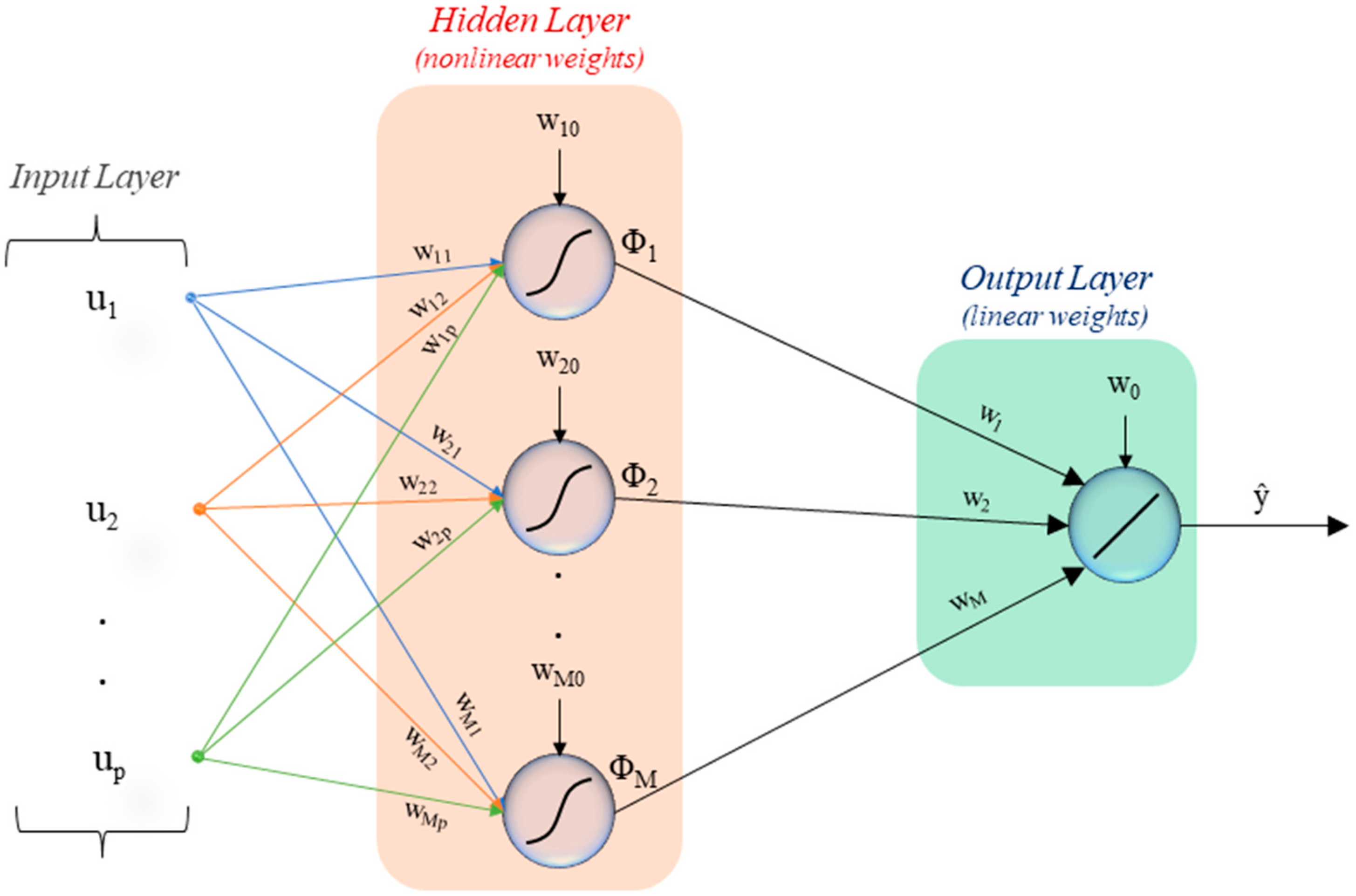
The structure of an ANN is shown in greater detail in Figure 3. The input consists of p input neurons (uj) forming the input layer. The middle layer, known as the hidden layer, contains a basis function and M neurons. The output neuron constitutes the output layer, of which there may be more than one, consisting of a linear sum function of all the contributions from neurons in the hidden layer corresponding to this output, multiplied by their output weights (wi), which are linear parameters [29].
The output neuron usually consists of a linear combination of the signals from the neurons in the hidden layer, with the addition of a bias (w0) whose value is normally 1. The output neuron determines the scale of the response and the point of operation of the neural network [29].
One of the most widely used neural networks is the multilayer perceptron (MLP), which is a feedforward network that uses the classical backpropagation algorithm for training the network and adjusting the weights. The perceptrons correspond to the hidden layer neurons, where a nonlinear activation function evaluates the input signals and their corresponding weights (plus one bias). The activation function may be of the logistic or hyperbolic tangent types [29].
Equation (30) shows the response of a base formulation of an MLP model for a hidden layer with n perceptrons connected to an output neuron and with defined inputs. The parameters wi and wij are the weights or parameters of the output layer and the hidden layer, respectively; M is the total number of parameters of the neural network; and p is the number of inputs u.
y ^ = i = 0 M w i Φ i j = 0 p w ij u j ,   Φ 0 = 1   and   u 0 = 1
There are two types of parameters or weights in this neural network, namely the nonlinear parameters of the perceptrons, which determine the direction, position, and slope of the activation function, and the linear parameters of the output layer, which only perform the scaling of the signals from the hidden layers. The training of an MLP neural network is achieved by optimizing the weights of the network, for which the backpropagation algorithm is widely used.
The neural networks were applied using the neural network toolbox in Matlab. The experimental input data and the output (target) data for each network were fed as described by Beale et al. [33]. One of the four graphical user interfaces (GUIs) was used in the function fitting mode, with fitting of the neural network to the data enabling prediction of the results. The neural network structure included a certain number of inputs, perceptrons of the hidden layer (only one hidden layer for all the developed networks) selected according to the performance of the neural network, and one output. This was a feedforward network, where the neurons in the hidden layer had a sigmoidal function and the neurons in the output layer were linear.

2.2.1. Training, Validation, and Testing of the Neural Network

After providing the inputs and output for the neural network, selection was made of the number of samples to be used for training the network and, subsequently, for validation and testing. Training was performed using the extended Levenberg–Marquardt backpropagation algorithm, which combines the gradient descent and Gauss–Newton methods. The use of 70% of the samples for training and 15% each for validation and testing was suggested by Beale et al. [33], because these are default ratios for training, testing, and validation. Although these values may vary, the standard distribution was already convenient in this work due to the sample size of the available experimental data. It should be noted that the samples were randomly chosen by the algorithm itself during training of the neural network.
The number of neurons was defined based on evaluation of the performance of the neural network. When the training was not satisfactory, it was necessary to increase the number of neurons until significant improvement was observed in the performance of the neural network. On the other hand, if the response started to show overfitting (low performance in the neural network testing stage), the number of neurons had to be reduced until an optimal value that provides satisfactory performance and a suitable response was reached.

2.2.2. Neural Network Performance Assessment

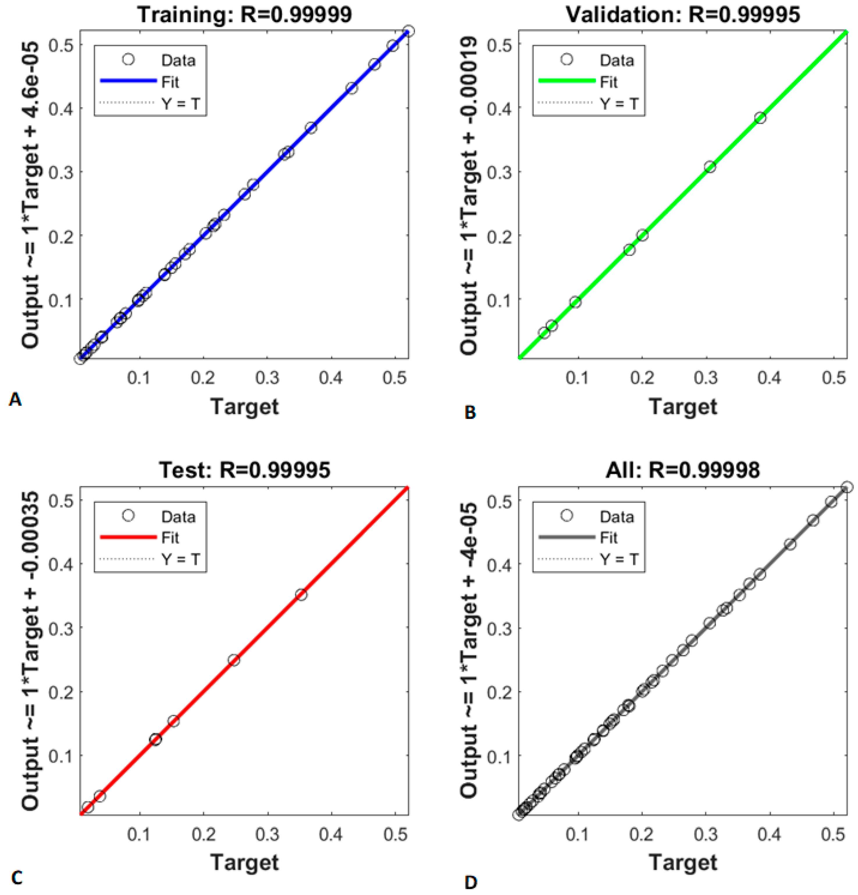
After the creation of a network, its performance was evaluated in several ways. The main result was given by the mean squared error (MSE) between the output of the neural network and the experimental values (targets), where a smaller value reflected a better result, with a smaller difference between the neural network response and the experimental value. The neural network was also evaluated using the values and graphs obtained via regression between the network outputs and the targets, where a regression coefficient (R) value closer to unity indicated greater accuracy of the neural network in describing the experimental values. The MSE and R values were both obtained for the neural network training, validation, and testing steps.
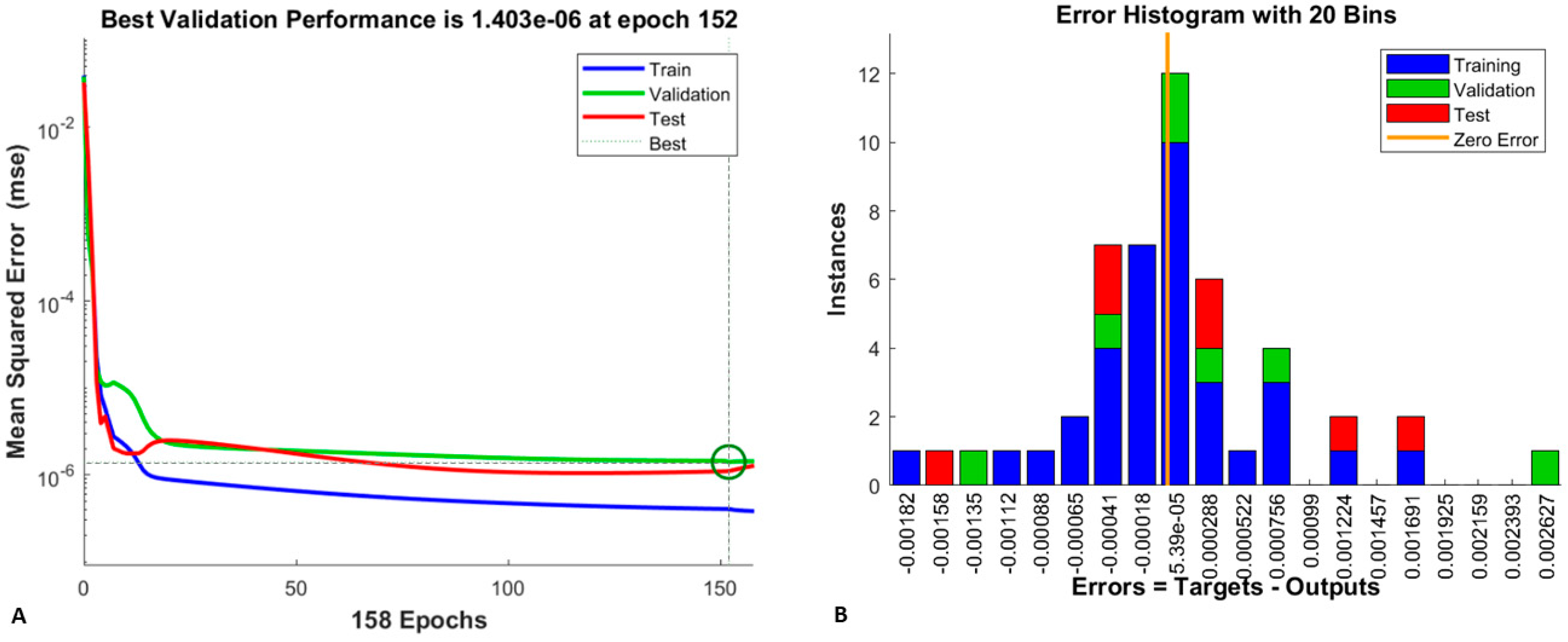
Additional graphs were also used to assist in evaluating the neural network performance, including error histograms for the training, validation, and test samples, allowing for the identification of possible outlier values that the network was unable to describe. A graph of network performance during the course of the iterations enabled identification of the best validation value and the iteration in which it occurred.
After the optimal number of perceptrons were defined, several ANNs were tested due to the random nature of the sampling selection, with the results being saved for later evaluation and reproduction. The most suitable network was chosen based on the best performance and the regression values for training, validation, and testing, as well as on the response of the neural network when compared to the sample data.

2.2.3. Neural Network for Polarization Curves of PtAg/C and PtAg/MnOx/C Electrodes at 60 °C and 90 °C

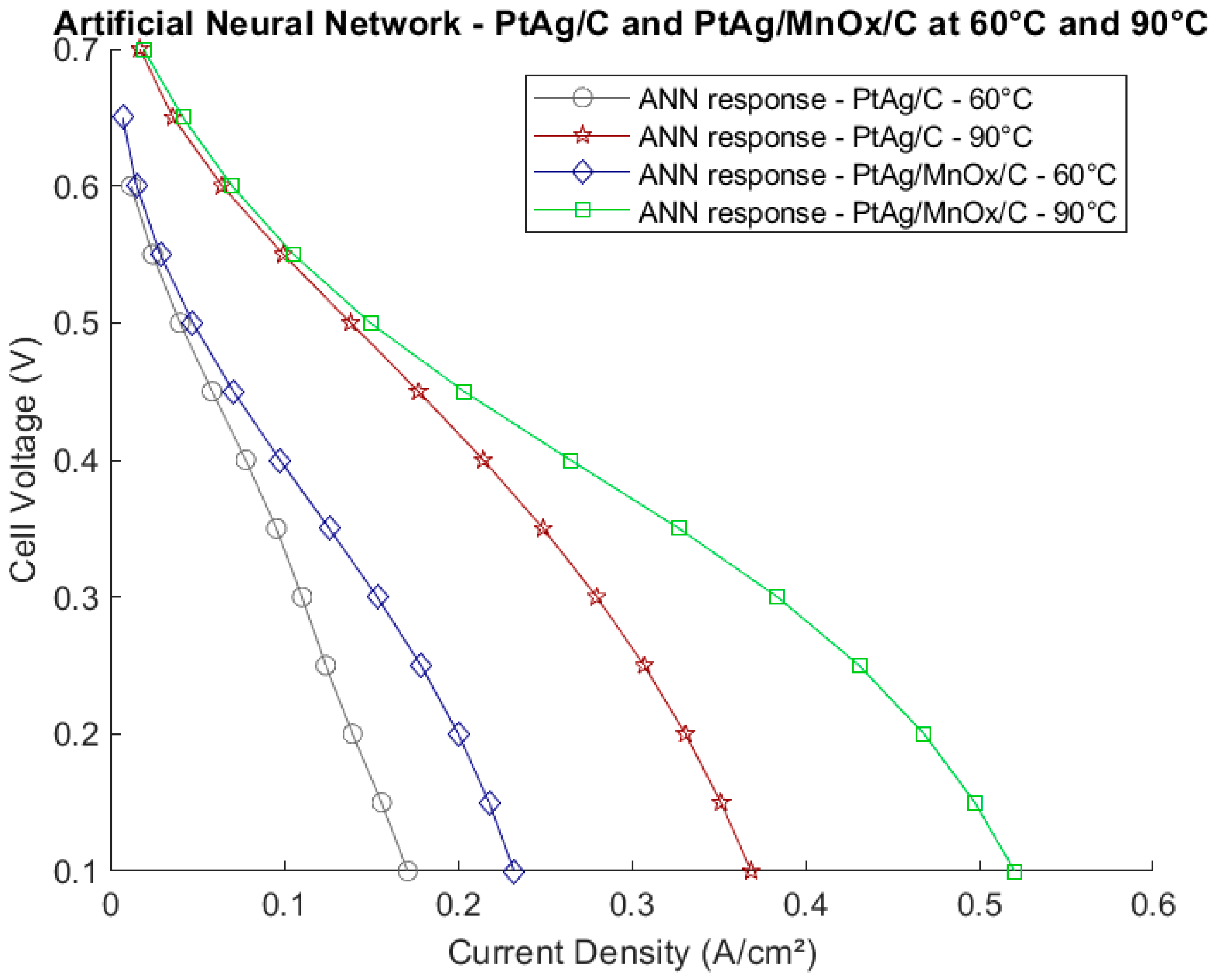
This network incorporated data from two different catalysts from those considered in the phenomenological models, namely the PtAg/C and PtAg/MnOx/C electrodes, which were also studied by Garcia et al. [28], at temperatures of 60 °C and 90 °C. The input layer was composed of 3 inputs: cell potential (Vcel), temperature, and absence or presence of MnOx (indicated by values of zero and unity, respectively). The output was the current density (i) in the cell. The procedure for obtaining the optimal number of neurons in the network was performed as described previously. In this case, the recommendation of Beale et al. [33] was adopted, with the distribution of samples being 70% for the training set, 15% for the validation set, and 15% for the test set.

3. Results and Discussion

This section presents the results obtained for the phenomenological and neural network models developed in the present work.

3.1. Phenomenological Models

Each phenomenological model is fully treated in a separate section below, except for the simplified phenomenological models, which are considered in the same section since they derived from the complete phenomenological model for the temperature of 60 °C.

3.1.1. Phenomenological Model at 60 °C

The results are presented below for the complete phenomenological model obtained using a temperature of 60 °C and the Pt/C electrode.

Polarization Curve

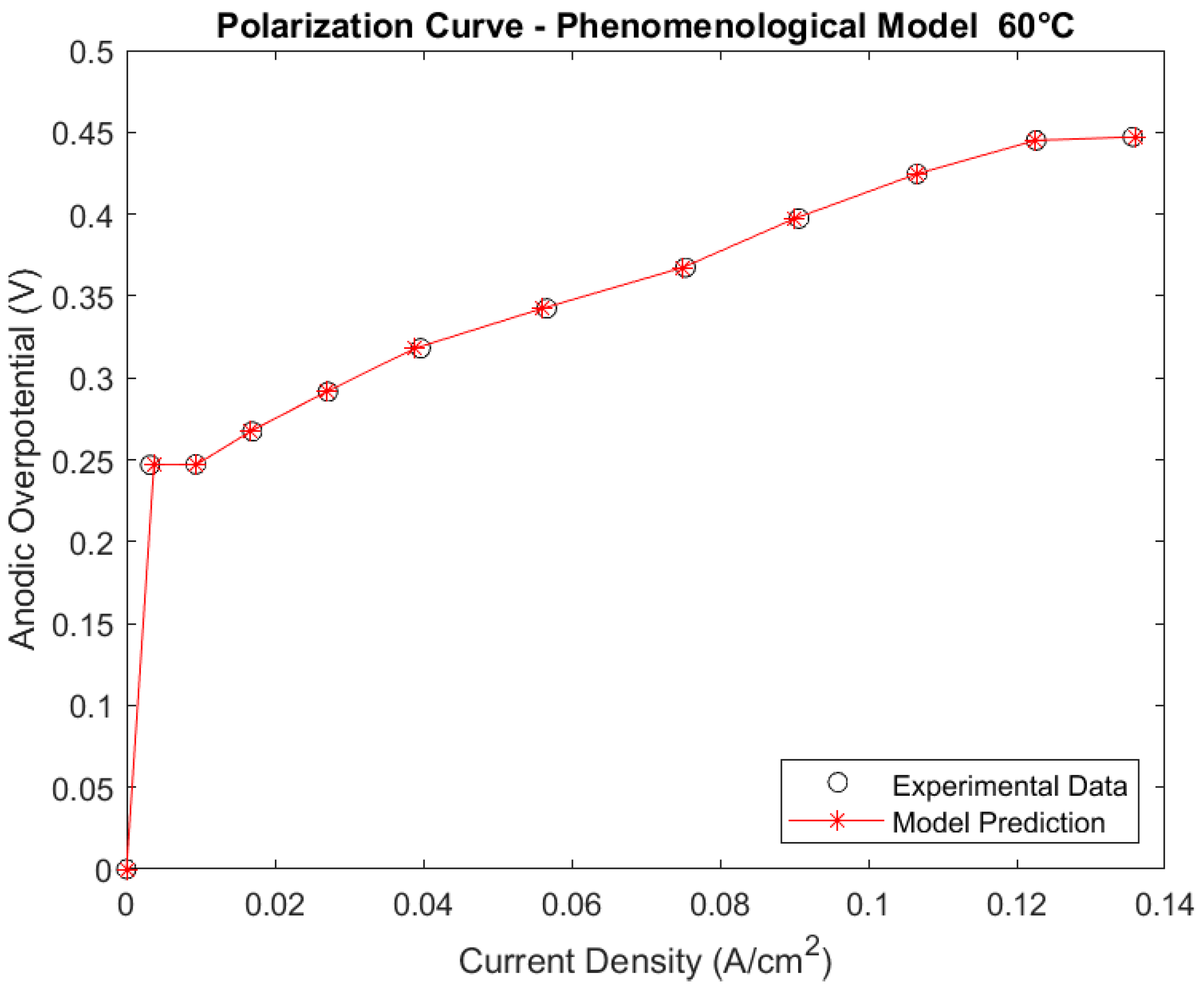
The polarization curve for the phenomenological model (PM) with a Pt/C electrode at 60 °C, is shown in Figure 4. It can be seen that the fit of the model (red) to the experimental data (black) was very precise, as shown statistically by the SSE and RMSE values of 192.03 (A/m2)2 and 4.00 A/m2, respectively. The RMSE provides an indication of the variability of the model response, so since the RMSE was very small, compared to the working range of the model (0–1357 A/m2), it was evident that the proposed model could provide reliable data prediction.

Catalyst Coverage Distribution

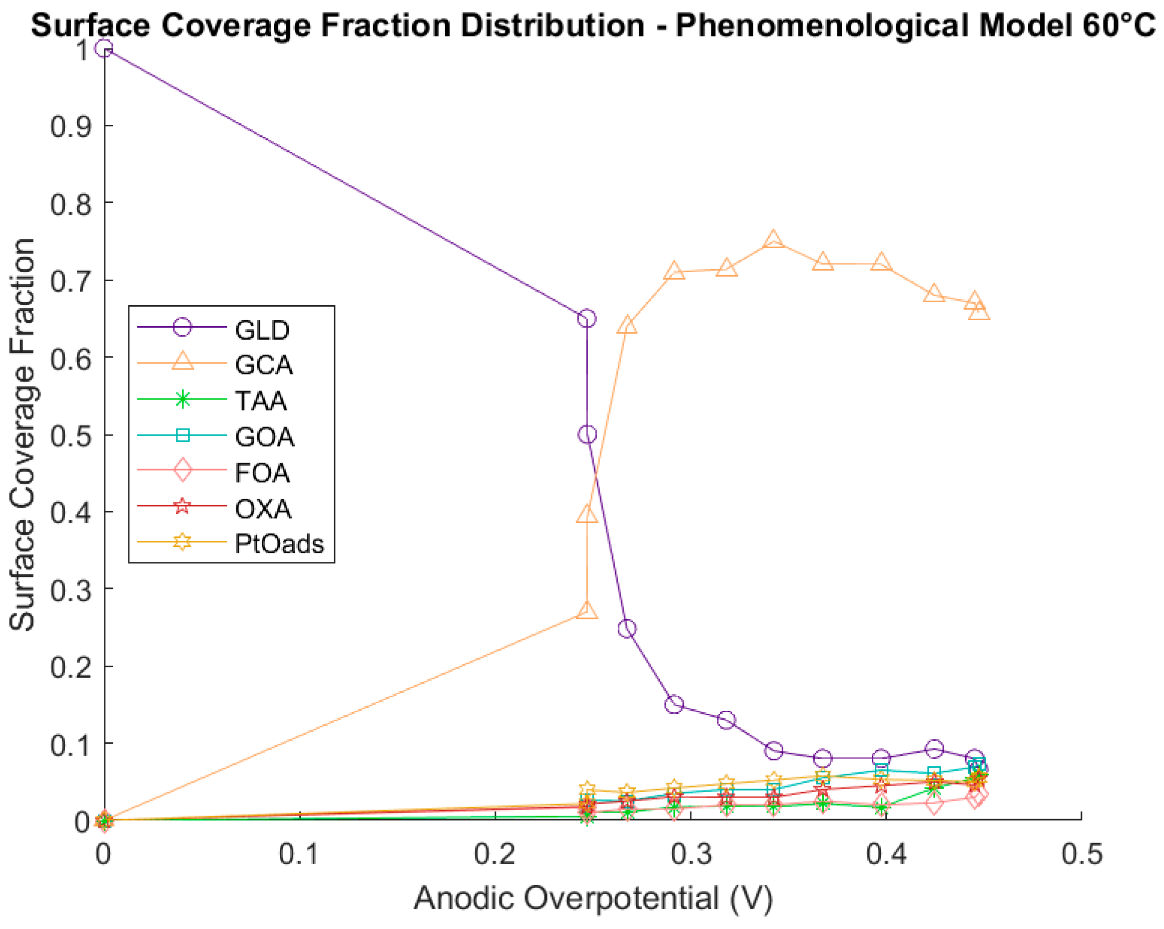
Figure 5 shows the coverage fraction distribution for the intermediates adsorbed on the catalyst, obtained using the fmincon function. After fitting the polarization curve, the distribution of adsorbed intermediates for this base case was in agreement with the literature, precisely following the products’ selectivity behavior (which is directly related to the coverage) shown in the work by Kwon et al. [3]. More specifically, while selectivity for glyceraldehyde decays from 100 to 10% as the potential increases, selectivity for glyceric acid increases, and the selectivities for the other intermediates generally remain below 10%. The same behavior is observed in Figure 5 (with the only difference being that in the model, the reaction pathway for the minor oxidation of the secondary hydroxyl of glycerol was neglected). Additionally, intermediates and products considered in the model are in complete accordance with the main products experimentally identified in previous works from the research group [1,28].
It should be noted that during the fitting, the lower and upper limits of the coverage fractions varied in relatively narrow ranges. This way, it was rational to consider that, in the end, the coverage fractions tended towards assumed values (instead of being adjustable within wide ranges for its determination). Nonetheless, the final values for the coverage fractions, derived from a meticulous search carried out during the fitting process, were based on reliable comparison with selectivity information reported in the literature.
Glyceraldehyde was an unstable intermediate formed during oxidation of the primary hydroxyl of glycerol, being rapidly consumed to produce glyceric acid as the overpotential increased. Glyceric acid was the most abundant adsorbed intermediate, with its selectivity remaining high even when consumed to form tartronic acid. The fractions of the latter and the other acids considered (glycolic, formic, and oxalic), as well as the fraction of Pt-Oads, were very low at smaller overpotentials, with their values generally remaining below 0.1.

Statistical Study of the Parameters

As described in the methodology section, for the fits shown in Figure 4 and Figure 5, all the parameters (coverage fractions, kinetic constants, and transfer coefficients) were included in the fitting using the fmincon function. For statistical study of the kinetic parameters in a new fitting process, the values of the coverage fractions were fixed (for the reasons discussed above), with the exception of the Pt-Oads fraction, because rounding errors when fixing this fraction (together with all the others) led to the optimization converging towards a region that did not satisfy the constraints (unfeasible area). Leaving this fraction varied did not influence the parameterization results but allowed for resolution of the numerical issue. Furthermore, in practice, there was no significant change in the value of this fraction during the course of the simulations. Table 2 shows the fitted values for the kinetic parameters with greatest impacts in the model (the most sensitive parameters), which presented the lowest values of SE, SD, and deviation magnitude, considering the coverage fractions as fixed parameters.
The kinetic constant k2 and the transfer coefficient α2 were associated with the consumption of glyceric acid and formation of tartronic acid, while the kinetic constants k5 and k5′, together with the transfer coefficient α4, were related to the dissociative adsorption of water and formation of the Pt-Oads active sites, in forward and reverse reaction directions. Also, it is worth noting that the values of the charge transfer coefficients were feasible from an electrochemical point of view, since these coefficients (which generally have values between 0 and 1) are already multiplied by the number of electrons exchanged (which for all reactions of the model is 2 electrons) and thus are within the allowed range, between 0 and 2.
The lower sensitivity parameters were fixed, since they had no significant impact on the model, showing that their values could vary greatly without affecting the response of the model. Hence, the values for these parameters are only assumed values.

Parameter Sensitivity

Figure 6A–C shows graphs for the parameter sensitivity tests, where the most sensitive kinetic constants were increased by multiplying by three different factors (1.1, 1.5, and 1.8) one at a time while the effect on the model result was observed in comparison with the original model response curve (black asterisks) and the experimental data (red circles). The kinetic constant k5 was the most sensitive, followed by k2 and then k5′, with almost an order of magnitude difference based on the deviation magnitude values. The k4 constant, which was one of the non-significant constants, was included in the graphs to demonstrate that it would not influence the model response, as in fact was observed.
The curves for the PM response with increase of constants k2 and k5 remained almost parallel to each other, with only modest differences as the multiplication factor was increased. This could be explained by the fact that both reactions were oxidation processes involving the release of two electrons, so it was expected that they would have similar effects on the model response. However, the graphical presentation confirmed the order of sensitivity indicated by the SD and deviation magnitude values, since the polarization curve with increased k5 showed slightly greater sensitivity to alteration of the parameter value.
When the values of the constants k2 and k5, corresponding to the oxidation reactions, were increased, the model response indicated a higher current density value for the same overpotential, while the opposite was also true, with a reduction in the overpotential for the same current density. This could be explained by the fact that increasing the values of these constants would increase the reaction rate, which would release more electrons and consequently increase the current density. In the case of constant k5′, which was related to a reduction reaction, an increase in its value led to an increase in the overpotential for the same current density and vice versa. Similar behavior was observed by de Oliveira et al. [25] in a study of ethanol oxidation in fuel cells.
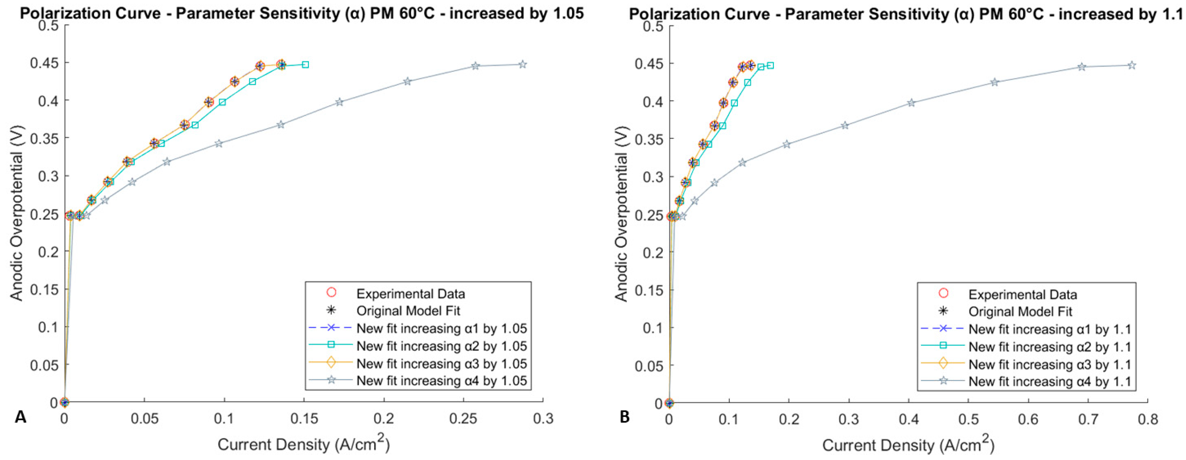
For the purpose of comparison, parametric sensitivity analysis was also performed with the transfer coefficients (Figure 7A,B). For better visualization, the transfer coefficients were increased 1.1-fold. Since there were few of these coefficients, they were all included in the analysis. In agreement with the deviation magnitude values (Table 2), the graphs show the same order of sensitivity of these kinetic parameters, with α4 having the greatest impact on the model, followed by α2. Parameters α1 and α3 showed no sensitivity, as expected.
Increases of α2 and α4 again resulted in increase of the current density for the same overpotential, especially in the case of α4.

Impact of the Most Sensitive Parameters on the Coverage Fraction Distribution

Figure 8A–D shows a comparison of the coverage fraction distribution for the full PM at 60 °C and three other distributions where the curves were modified due to the increases of the most sensitive kinetic constants by factors of 1.5, 5, and 10. The changes in the selectivities could be explained by the faster reaction rates when the values of the constants were increased, with concomitant increase of the current density response. Hence, refitting of the polarization curves to the experimental data required alteration of the coverage in order to compensate for the shift towards higher current density in the model, such that the selectivity of the intermediates in general decreased. For this to occur, the selectivity of the unstable glyceraldehyde intermediate should increase, while there should be a decrease of Pt-Oads coverage, since this determined the quantity of available reaction sites at which the compounds were formed.

3.1.2. Simplified Models 1 and 2

For the first simplified phenomenological model (SPM1), oxalic acid (AOX) was removed based on consideration of the compounds that could not be removed from the reaction, such as the products with the greatest coverage of the catalyst (glyceraldehyde and glyceric acid) as well as the compounds whose formation was associated with the most sensitive kinetic constants (k2, for formation of tartronic acid, and k5 and k5′, for formation of the Pt-Oads active sites). There then remained the products formed in the reactions related to the kinetic constants k3 and k4. In SPM1, it was decided only one product would be removed, with oxalic acid being chosen due to the codependency between the products of these two reactions (since oxalic acid was produced via the oxidation of glycolic acid). With the removal of k4, there was also removal of desorption constant k4″ and transfer coefficient α3 from the simulation, consequently reducing the number of kinetic parameters from seventeen to fourteen.
For the second simplified phenomenological model (SPM2), selection of the products to be removed was made in the same way described above, but this time the compounds glycolic acid, formic acid, and oxalic acid were removed, resulting from the reactions related to kinetic constants k3 and k4. Thus, desorption constants k3″, k3‴, and k4″ were also removed in addition to transfer coefficient α3, which reduced the number of adjustable kinetic parameters from seventeen to eleven. It should be noted that the reaction for formation of glycolic acid and formic acid did not involve the release of electrons, so there was no associated transfer coefficient.

Polarization Curves

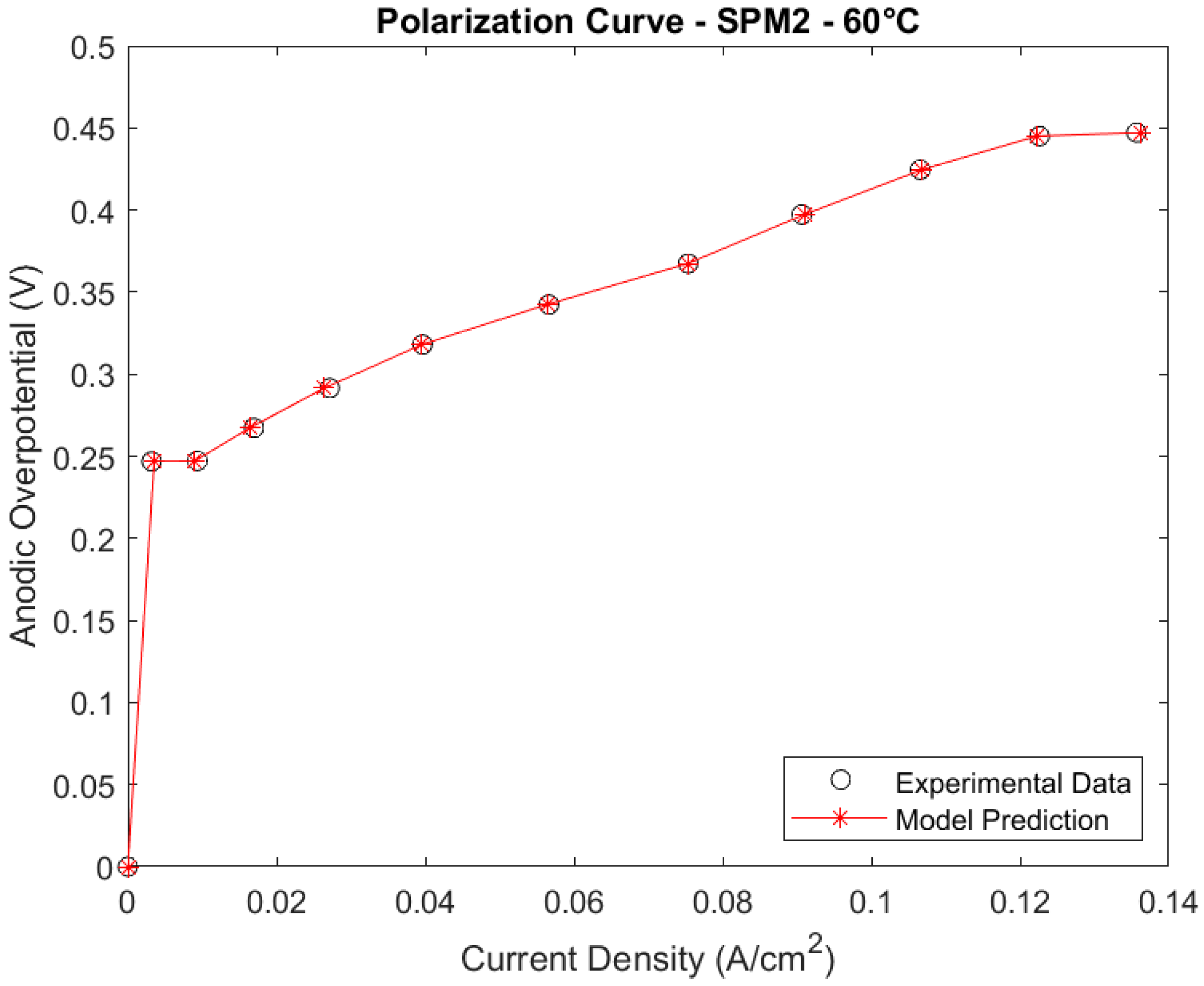
For SPM1, the SSE and RMSE were 149.10 (A/m2)2 and 3.52 A/m2, respectively, with these values and the polarization curve indicating an excellent fit of the model to the experimental data. For SPM2, the SSE and RMSE values were 195.81 (A/m2)2 and 4.04 A/m2, respectively, and again there was an excellent fit of the polarization curve (Figure 9). The low variability of the model responses was supported by the RMSE values obtained for the two models, which were very small, relative to the working range of the cell (0-1357 A/m2).

Catalyst Coverage Distributions

For SPM1, the coverage distribution remained very similar to that observed for the full model, which could be explained by the fact that the removal of only one product did not significantly influence the distribution for the other compounds, since the oxalic acid fraction in the full model did not exceed 0.1.
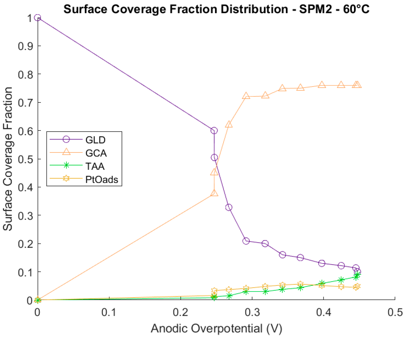
For SPM2 (Figure 10), the coverage distribution differed from that for the full model, but followed the same logic for formation of the products. The removal of three products significantly affected distribution, with the tartronic acid fraction showing the greatest increase, while the fraction of Pt-Oads active sites remained almost constant at high overpotentials.

Statistical Study of the Parameters

Table 3 and Table 4 show the SE, SD, and deviation magnitude values for the most sensitive constants of the SPM1 and SPM2 models, respectively.
For both simplified models, the most significant constants were the same as for the full model, with only the deviation values being different (as expected, since only products of the reactions related to the less influential parameters were removed). The fitted values remained similar, with only transfer coefficient α4 showing a slight change in order to fit the current to the experimental data.
For SPM1, there was already an indication that the sensitivity of constant k2″ (tartronic acid desorption) could have greater importance. In fact, for SPM2, the deviation magnitude of this constant demonstrated relevant sensitivity. However, this parameter was not incorporated into the current density equation (Equation (28)), so its alteration did not directly affect the polarization curve. Nonetheless, calculation of the statistical values used the Hessian matrix, estimated using the fmincon function of Matlab. This estimate was the Hessian of the Lagrangian associated with the constrained optimization problem, which, in addition to the objective function (current density/polarization curve), incorporated its specific equations for the constraints (balances of conservation of the adsorbed species). Hence, the increased sensitivity of k2″ in the simplified models was an indirect effect resulting from estimation of the Hessian via the Lagrangian.

3.1.3. Comparison between the Full Model at 60 °C and Simplified Models 1 and 2

Table 5 shows the relative deviation values (deviation magnitude) for the most significant kinetic parameters of the full PM, SPM1, and SPM2 models. The deviation magnitudes of almost all the parameters were lower for the simplified models compared to the full PM. This was expected, since reducing the number of adjustable parameters via the removal of products should lead to smaller deviation values for the parameters retained in the fitting.
The simplified SPM1 and SPM2 models revealed the versatility of the proposed full phenomenological model for the most common Pt/C electrode type at a moderate temperature (60 °C), where the removal of one or more products did not affect the ability of the models to fit the experimental data. It could therefore be concluded that it was possible to obtain satisfactory simplified models from a more complete general model.

3.1.4. Phenomenological Model at 90 °C

The results for the PM with the Pt/C electrode at 90 °C are discussed below.

Polarization Curves

Figure 11 shows the polarization curve for the full PM with the Pt/C electrode at 90 °C. The fitted SSE and RMSE values were 166.44 (A/m2)2 and 3.60 A/m2, respectively, indicating that the proposed model provided a good description of the experimental data, with low variability in the model response, since the RMSE value was very small compared to the working range of the cell at 90 °C (0–2982 A/m2).

Catalyst Coverage Distribution

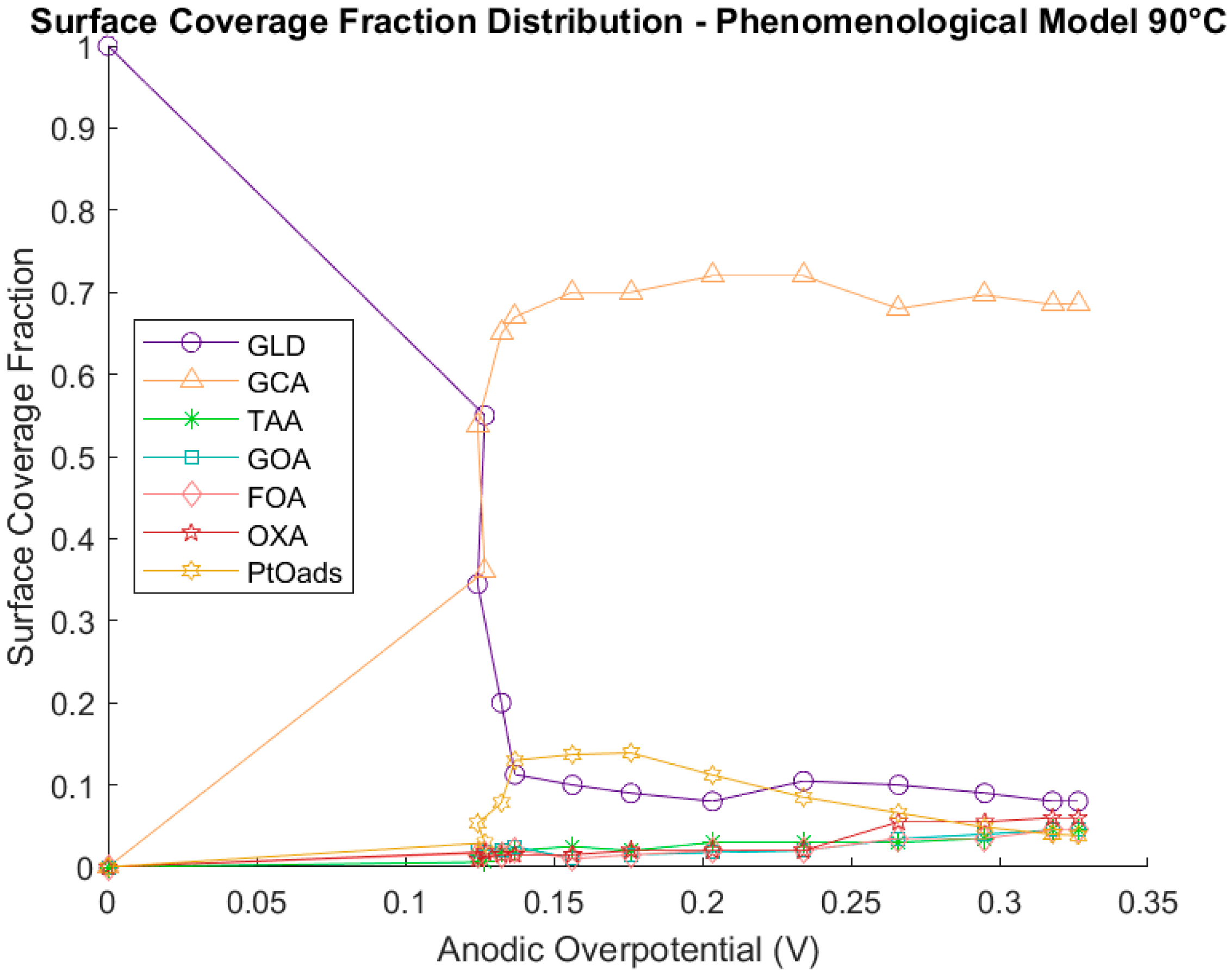
Figure 12 shows the coverage fraction distribution of the adsorbed intermediates for the full phenomenological model with the Pt/C electrode at 90 °C. Analogously to the full PM, SPM1, and SPM2 at 60 °C, the distribution of intermediates was in line with the behavior reported in the literature. Glyceric acid was the most predominant compound at medium and high overpotentials, together with smaller fractions of other compounds, including glyceraldehyde, whose selectivity decreased rapidly as it was consumed. The fractions of the other compounds mostly remained below 0.1, with the exception of the Pt-Oads coverage fraction, which was slightly higher at medium overpotentials and then decreased to the same order of magnitude as the fractions for the other compounds.
Similar to the full PM at 60 °C, as the parameter fitting process progressed, the coverage fractions converged in relatively narrow ranges in terms of the lower and upper limits, so the values were subsequently considered fixed (as already discussed).

Statistical Study of the Parameters

In the same way as for the previous phenomenological models, the initial fitting of this model included all the coverage fractions of the intermediates and the kinetic parameters as adjustable variables, with the coverage fractions being fixed in the statistical study. In this case, unlike the previous models, the glyceric acid coverage fraction was left as an adjustable parameter due to numerical issues. The fitted values for the most sensitive kinetic parameters are shown in Table 6, together with the corresponding SE, SD, and deviation magnitude values.
Similar to the phenomenological models treated previously, the kinetic parameters identified as having the greatest impact in the model were k2 and α2, associated with the consumption of glyceric acid and the production of tartronic acid, and k5, k5′, and α4, associated with the formation of Pt-Oads active sites via dissociative adsorption of water. The order of sensitivity was also similar, with k5 being the most sensitive kinetic constant, followed by k2 and k5′, while the most sensitive transfer coefficient was α4, followed by α2. It is noteworthy that α4 was the most sensitive parameter in all the phenomenological models considered so far. Even without use of the complete subset selection method, it was possible to obtain the values and deviations of these parameters, with the results showing that despite the increase of the process temperature, the most significant model parameters remained the same.

3.1.5. Additional Validation of PMs at 60 °C and 90 °C

Since the modeling results presented in Figure 4 and Figure 11 fitted very well with experimental data with very small error, additional information about validation is available in Figure 13, showing that interpolation obtained from the models (i.e., for data points not used directly to fit the model parameters) are smooth and coherent with the experimental trends (this smoothness confirming the absence of overfitting issues).

3.2. Neural Network for the PtAg/C and PtAg/MnOx/C Electrodes at 60 °C and 90 °C

For the neural network considering the reaction data obtained with the PtAg/C and PtAg/MnOx/C electrodes at temperatures of 60 °C and 90 °C, the optimal number of perceptrons found was 6 neurons in a single hidden layer. Above this number, no improvement of performance was observed, while worsening of the regression and MSE values occurred above 10 neurons. No overfitting was observed in the ANN, although it was estimated that this could occur if the number of perceptrons was increased further.
Figure 14A–D shows the regression values for the training, validation, and testing steps of the network development together with the regression of all the sample values. The MSE values for the network training, validation, and testing steps were 4.04 × 10⁻⁷, 1.40 × 10⁻⁶, and 1.11 × 10⁻⁶ (A/cm2)2, respectively, and the value for the global performance of the ANN was 6.47 × 10⁻⁷ (A/cm2)2. The network RMSE value was 0.08 A/m2. The regression between the network outputs and the targets showed that the neural network provided excellent prediction of the experimental values, since a perfect relationship was obtained for the training step, while values close to unity were also obtained for the validation and testing steps. In a few words, the performance was good not only for training data but also for validation and testing, indicating no overfitting issues.
Figure 15 shows the responses of the neural network model. Compared to the experimental data presented in Garcia et al. [28], agreement is full. Additionally, a smooth potential–current behavior is observed, confirming the absence of overfitting issues. The use of neural networks to predict the behavior of oxidation reactions in a fuel cell that uses more complex electrodes is of great importance, since it enables representation of the functional dependence between cell potential and current density in such cases, where it would be currently unfeasible to develop complete mechanistic models capable of accurately describing all the mechanisms involved. Even the PtAg/C bimetallic electrode (for glycerol oxidation) presents greater mechanistic complexity compared to the Pt/C electrode due to the presence of silver, and the complexity increases further for oxidation performed using the PtAg/MnOx/C electrode. In these cases, where the mechanisms are highly complex, ANNs can provide a prediction of the functional relationships among the variables involved [34]. Alternatively, another approach would be to describe the kinetics of the bimetallic catalyst via one single set of phenomenological rate constants without taking into account differences in the distinct adsorption and reaction sites [16,23].
Figure 16A shows the performance of the ANN during the iterations, where the best MSE value for validation was obtained in the 152nd iteration. For the training step, the MSE always decreased, while for the testing step, the MSE started to increase slightly after reaching the best validation performance. Figure 16B shows the error histogram, which presents convenient distribution (Gaussian-like behavior).
The results indicated the effectiveness of neural networks for describing the oxidation processes in a DGFC, especially in the case of more complex mechanisms that still cannot be completely described by mechanistic models, such as when using PtAg/C and PtAg/MnOx/C electrodes.

3.3. Pros and Cons of the Developed Models

In this section, two tables (Table 7 for phenomenological models and Table 8 for ANNs) are presented with the pros and cons of the developed models; the tables also refer to the advantages and disadvantages presented in the literature, aiming at a better presentation/coverage of the problem and development.

4. Conclusions

The proposed mechanistic model was shown to be highly robust in describing the mechanism and the experimental data, with all the developed phenomenological models providing excellent fits, obtaining low RMSE values and descriptions of the catalyst coverage in line with experimental data reported in the DGFC literature.
The kinetic parameters with the greatest impacts on the model response were k2, k5, k5′, α2, and α4, where k2 and α2 relate to the reaction of glyceric acid consumption and formation of tartronic acid, while k5, k5′, and α4 relate to the dissociative adsorption of water and formation of the Pt-Oads active sites (forward reaction) and OH desorption (reverse reaction). All the developed phenomenological models showed the same kinetic parameters as being the most sensitive.
Parametric sensitivity analysis showed that increases of kinetic constants k2 and k5 led to decreases in the overpotential, with consequent increases of the current density, since they were related to oxidation reactions (with the release of electrons). The opposite occurred with increase of constant k5′, which was related to a reduction reaction (with the consumption of electrons).
The readjustment of the model by increasing the values of the most sensitive kinetic constants led to an increase in the glyceraldehyde coverage fraction and reductions in all the others. Changes in the profile of adsorbed intermediates, resulting from changes in the values of the parameters with greatest impacts, provided additional insight into the influence of the model parameters on the degree of catalyst coverage (and vice versa). However, the general (qualitative) behavior of the coverage fractions remained essentially the same and was consistent with the literature.
The findings showed the versatility of the complete mechanistic model proposed here for a simple Pt/C electrode, where the removal of one or more products in SPM1 and SPM2 did not affect the fit of the model, demonstrating the feasibility of obtaining excellent simplified models from a more complete general model. Additionally, from a wider perspective, although the general model brought here can be already considered complete, additional intermediates and products can still be incorporated into the reaction mechanism, e.g., glyoxylic acid (but this is beyond the scope of this paper).
Increase of the temperature used in the phenomenological model resulted in changes in the values of some of the constants, especially for the most significant parameters, where the values of k2, α2, and α4 increased, the value of k5 remained the same, and the value of k5′ decreased, reflecting a shift of the equilibrium towards the formation of Pt-Oads sites. The values of the other non-sensitive constants generally remained (coherently) unchanged.
The neural network model developed in this work showed an excellent fit to the experimental data for all the systems evaluated, as shown by the performance and regression data. These models are extremely important for predicting the behavior of complex mechanisms that cannot yet be feasibly described by phenomenological models, such as those associated with use of the PtAg/C and PtAg/MnOx/C electrodes studied in the present work. Artificial neural networks enable representation of the functional interdependence between input variables and the cell current density, for cases that would be too complex for application of mechanistic modeling.

Author Contributions

Conceptualization, A.P., U.J.d.C., D.S.B.L.d.O., G.T.-F. and R.d.S.J.; formal analysis, A.P., U.J.d.C., D.S.B.L.d.O., G.T.-F. and R.d.S.J.; funding acquisition, R.d.S.J.; investigation, A.P. and U.J.d.C.; methodology, A.P., U.J.d.C., D.S.B.L.d.O., G.T.-F. and R.d.S.J.; project administration, R.d.S.J.; resources, R.d.S.J.; software, A.P., U.J.d.C., D.S.B.L.d.O. and R.d.S.J.; validation, A.P. and R.d.S.J.; visualization, A.P. and R.d.S.J.; writing—original draft, A.P. and R.d.S.J.; writing—review and editing, A.P., U.J.d.C., D.S.B.L.d.O., G.T.-F. and R.d.S.J. All authors have read and agreed to the published version of the manuscript.

Funding

This study was financed in part by the Coordenação de Aperfeiçoamento de Pessoal de Nível Superior—Brazil (CAPES)—Finance Code 001.

Data Availability Statement

Sources for all data used in this work were cited along the text.

Conflicts of Interest

The authors declare no conflict of interest.

Abbreviations

List of Symbols
E0 open circuit potential (V or mV)
Vcel cell potential (V or mV)
η overpotential (V or mV); subscripts indicate anodic (A) and cathodic (C); conc: concentration
F Faraday constant (96,845 C/mol e)
R ideal gas constant (8.3145 V·C/(mol·K))
T absolute temperature (K)
Cgly glycerol concentration (mol/m3)
i current density (A/m2 or A/cm2)
i0 exchange current density (A/m2 or A/cm2)
iL limiting current density (A/m2 or A/cm2)
Rmem membrane ohmic resistance (Ω·m2)
k reaction kinetic constants
α charge transfer coefficient
θi coverage fraction for adsorbed species i
n number of electrons
N number of sample data
H Hessian matrix
σ2 noise variance
wi output layer weights
wij hidden layer weights
ϕi hidden layer perceptrons output
y process output
ŷ model output
List of Abbreviations
AFCalkaline fuel cell
ANNartificial neural network
DEFCdirect ethanol fuel cell
DGFCdirect glycerol fuel cell
FOAformic acid
GCAglyceric acid
GLDglyceraldehyde
GLYglycerol
GOAglycolic acid
MLPmultilayer perceptron
MSEmean squared error
OXAoxalic acid
PBIpolybenzimidazole
PMphenomenological model
RMSEroot mean squared error
SAMFCsolid alkaline membrane fuel cell
SDstandard deviation
SEstandard error
SPEFCsolid polymer electrolyte fuel cell
SPM1simplified phenomenological model 1
SPM2simplified phenomenological model 2
SSEsum of squared errors
TAAtartronic acid

Appendix A

Formation of the corresponding salts (glycerate, tartronate, glycolate, formate, oxalate) in alkaline media.
C 3 H 8 O 3 + 2   OH C 3 H 6 O 3 ads + 2 H 2 O + 2   e k 0
C 3 H 6 O 3 ads C 3 H 6 O 3 k 0
C 3 H 6 O 3 ads + PtO ads + OH C 3 H 5 O 4 ( ads ) + H 2 O   k 1
C 3 H 5 O 4 ( ads ) C 3 H 5 O 4 k 1
C 3 H 5 O 4 ( ads ) + PtO ads + 3   OH C 3 H 2 O 5 ( ads ) 2 + 3 H 2 O + 2   e k 2
C 3 H 2 O 5 ( ads ) 2 C 3 H 2 O 5 2 k 2
C 3 H 5 O 4 ( ads ) + PtO ads + OH C 2 H 3 O 3 ( ads ) + CH O 2 ( ads ) + H 2 O   k 3
C 2 H 3 O 3 ( ads ) C 2 H 3 O 3 k 3
CH O 2 ( ads ) CH O 2 k 3
C 2 H 3 O 3 ( ads ) + PtO ads + 3   OH C 2 O 4 ( ads ) 2 + 3 H 2 O + 2   e k 4
C 2 O 4 ( ads ) 2 C 2 O 4 2 k 4
2 OH PtO ads + H 2 O + 2 e k 5 ,   k 5

References

  1. Gomes, J.F.; Tremiliosi-Filho, G. Spectroscopic Studies of the Glycerol Electro-Oxidation on Polycrystalline Au and Pt Surfaces in Acidic and Alkaline Media. Electrocatalysis 2011, 2, 96–105. [Google Scholar] [CrossRef]
  2. Gomes, J.F.; Paula, F.B.C.; Gasparotto, L.H.S.; Tremiliosi-Filho, G. The influence of the Pt crystalline surface orientation on the glycerol electro-oxidation in acidic media. Electrochim. Acta 2012, 76, 88–93. [Google Scholar] [CrossRef]
  3. Kwon, Y.; Schouten, K.J.P.; Koper, M.T.M. Mechanism of the Catalytic Oxidation of Glycerol on Polycrystalline Gold and Platinum Electrodes. ChemCatChem 2011, 3, 1176–1185. [Google Scholar] [CrossRef]
  4. Roquet, L.; Belgsir, E.M.; Léger, J.-M.; Lamy, C. Kinetics and mechanisms of the electrocatalytic oxidation of glycerol as investigated by chromatographic analysis of the reaction products: Potential and pH effects. Electrochim. Acta 1994, 39, 2387–2394. [Google Scholar] [CrossRef]
  5. Wang, Y.; Li, L.; Hu, L.; Zhuang, L.; Lu, J.; Xu, B. A feasibility analysis for alkaline membrane direct methanol fuel cell: Thermodynamic disadvantages versus kinetic advantages. Electrochem. Commun. 2003, 5, 662–666. [Google Scholar] [CrossRef]
  6. Coutanceau, C.; Demarconnay, L.; Lamy, C.; Léger, J.-M. Development of electrocatalysts for solid alkaline fuel cell (SAFC). J. Power Sources 2006, 156, 14–19. [Google Scholar] [CrossRef]
  7. Behr, A.; Eilting, J.; Irawadi, K.; Leschinski, J.; Lindner, F. Improved utilisation of renewable resources: New important derivatives of glycerol. Green Chem. 2008, 10, 13–30. [Google Scholar] [CrossRef]
  8. Bianchi, C.L.; Canton, P.; Dimitratos, N.; Porta, F.; Prati, L. Selective oxidation of glycerol with oxygen using mono and bimetallic catalysts based on Au, Pd and Pt metals. Catal. Today 2005, 102–103, 203–212. [Google Scholar] [CrossRef]
  9. Zhang, Z.; Xin, L.; Li, W. Electrocatalytic oxidation of glycerol on Pt/C in anion-exchange membrane fuel cell: Cogeneration of electricity and valuable chemicals. Appl. Catal. B Environ. 2012, 119–120, 40–48. [Google Scholar] [CrossRef]
  10. Zhou, Y.; Shen, Y.; Piao, J. Sustainable Conversion of Glycerol into Value-Added Chemicals by Selective Electro-Oxidation on Pt-Based Catalysts. ChemElectroChem 2018, 5, 1636–1643. [Google Scholar] [CrossRef]
  11. Houache, M.S.E.; Hughes, K.; Baranova, E.A. Study on catalyst selection for electrochemical valorization of glycerol. Sustain. Energy Fuels 2019, 3, 1892–1915. [Google Scholar] [CrossRef]
  12. Garcia, R.; Besson, M.; Gallezot, P. Chemoselective catalytic oxidation of glycerol with air on platinum metals. Appl. Catal. A Gen. 1995, 127, 165–176. [Google Scholar] [CrossRef]
  13. Kimura, H. Selective oxidation of glycerol on a platinum-bismuth catalyst by using a fixed bed reactor. Appl. Catal. A Gen. 1993, 105, 147–158. [Google Scholar] [CrossRef]
  14. Kimura, H.; Tsuto, K.; Wakisaka, T.; Kazumi, Y.; Inaya, Y. Selective oxidation of glycerol on a platinum-bismuth catalyst. Appl. Catal. A Gen. 1993, 96, 217–228. [Google Scholar] [CrossRef]
  15. Gallezot, P. Selective oxidation with air on metal catalysts. Catal. Today 1997, 37, 405–418. [Google Scholar] [CrossRef]
  16. Worz, N.; Brandner, A.; Claus, P. Platinum−bismuth-catalyzed oxidation of glycerol: Kinetics and the origin of selective deactivation. J. Phys. Chem. C 2009, 114, 1164–1172. [Google Scholar] [CrossRef]
  17. Kwon, Y.; Birdja, Y.; Spanos, I.; Rodriguez, P.; Koper, M.T.M. Highly Selective Electro-Oxidation of Glycerol to Dihydroxyacetone on Platinum in the Presence of Bismuth. ACS Catal. 2012, 2, 759–764. [Google Scholar] [CrossRef]
  18. Ilie, A.; Simoes, M.; Baranton, S.; Coutanceau, C.; Martemianov, S. Influence of operational parameters and of catalytic materials on electrical performance of direct glycerol solid alkaline membrane fuel cells. J. Power Sources 2011, 196, 4965–4971. [Google Scholar] [CrossRef]
  19. Lobato, J.; Cañizares, P.; Rodrigo, M.A.; Piuleac, C.-G.; Curteanu, S.; Linares, J.J. Direct and inverse neural networks modelling applied to study the influence of the gas diffusion layer properties on PBI-based PEM fuel cells. Int. J. Hydrogen Energy 2010, 35, 7889–7897. [Google Scholar] [CrossRef]
  20. Sousa, R., Jr.; Gonzalez, E.R. Mathematical modeling of polymer electrolyte fuel cells. J. Power Sources 2005, 147, 32–45. [Google Scholar] [CrossRef]
  21. Simões, M.; Baranton, S.; Coutanceau, C. Electro-oxidation of glycerol at Pd based nano-catalysts for an application in alkaline fuel cells for chemicals and energy cogeneration. Appl. Catal. B Environ. 2010, 93, 354–362. [Google Scholar] [CrossRef]
  22. Milewski, J.; Szczęśniak, A.; Szabłowski, Ł.; Dybiński, O.; Miller, A. Artificial neural network model of molten carbonate fuel cells: Validation on experimental data. Int. J. Energy Res. 2019, 43, 6740–6761. [Google Scholar] [CrossRef]
  23. Sousa, R., Jr.; Anjos, D.M.; Tremiliosi-Filho, G.; Gonzalez, E.R.; Coutanceau, C.; Sibert, E.; Léger, J.-M.; Kokoh, K.B. Modeling and simulation of the anode in direct ethanol fuels cells. J. Power Sources 2008, 180, 283–293. [Google Scholar] [CrossRef]
  24. Maia, L.K.K.; Sousa, R., Jr. Three-dimensional CFD modeling of direct ethanol fuel cells: Evaluation of anodic flow field structures. J. Appl. Electrochem. 2016, 47, 25–37. [Google Scholar] [CrossRef]
  25. de Oliveira, D.S.B.L.; Colmati, F.; de Sousa, R., Jr. Reaction Kinetics-Based Modeling and Parameter Sensitivity Analysis of Direct Ethanol Fuel Cells. Energies 2022, 15, 9143. [Google Scholar] [CrossRef]
  26. Oliveira, D.S.B.L.; Colmati, F.; Gonzalez, E.R.; Sousa, R., Jr. Neurofuzzy modelling on the influence of Pt–Sn catalyst properties in direct ethanol fuel cells performance: Fuzzy inference system generation and cell power density optimization. Int. J. Hydrogen Energy 2023, 48, 24481–24491. [Google Scholar] [CrossRef]
  27. Han, X.; Chadderdon, D.J.; Qi, J.; Xin, L.; Li, W.; Zhou, W. Numerical analysis of anion-exchange membrane direct glycerol fuel cells under steady state and dynamic operations. Int. J. Hydrogen Energy 2014, 39, 19767–19779. [Google Scholar] [CrossRef]
  28. Garcia, A.C.; Ferreira, E.B.; Barros, V.V.S.; Linares, J.J.; Tremiliosi-Filho, G. PtAg/MnOx/C as a promising electrocatalyst for glycerol electro-oxidation in alkaline medium. J. Electroanal. Chem. 2017, 793, 188–196. [Google Scholar] [CrossRef]
  29. Nelles, O. Nonlinear System Identification—From Classical Approaches to Neural Networks and Fuzzy Models, 1st ed.; Springer: Berlin/Heidelberg, Germany, 2001. [Google Scholar]
  30. Boekel, M.A.J.S. Statistical Aspects of Kinetic Modeling for Food Science Problems. J. Food Sci. 1996, 61, 477–486. [Google Scholar] [CrossRef]
  31. MathWorks Inc. Constrained Nonlinear Algorithms. Help Center. 2022. Available online: https://www.mathworks.com/help/optim/ug/constrained-nonlinear-optimization-algorithms.html#brnox01 (accessed on 5 August 2022).
  32. Pinto, G.A. Biorefinaria de Soro de Queijo: Engenharia de Bioprocessos e Sistemas Aplicada à Transformação de um Resíduo Poluente em Produtos com Valor Agregado [Cheese Whey Biorefinery: Bioprocess and Systems Engineering Applied to the Transformation of a Pollutant Waste into Value-Added Products]. Ph.D. Thesis, Universidade Federal de São Carlos, São Paulo, Brazil, 2008. (In Portuguese). [Google Scholar]
  33. Beale, M.H.; Hagan, M.T.; Demuth, H.B. Neural Network Toolbox™: User’s Guide, 7th ed.; Mathworks: Natick, MA, USA, 2010. [Google Scholar]
  34. Sousa, R., Jr.; Colmati, F.; Gonzalez, E.R. Modeling techniques applied to the study of gas diffusion electrodes and proton exchange membrane biochemical fuel cells. J. Power Sources 2006, 161, 183–190. [Google Scholar] [CrossRef]
  35. Demirel, S.; Lucas, M.; Wärnå, J.; Salmi, T.; Murzin, D.; Claus, P. Reaction kinetics and modelling of the gold catalysed glycerol oxidation. Top. Catal. 2007, 44, 299–305. [Google Scholar] [CrossRef]
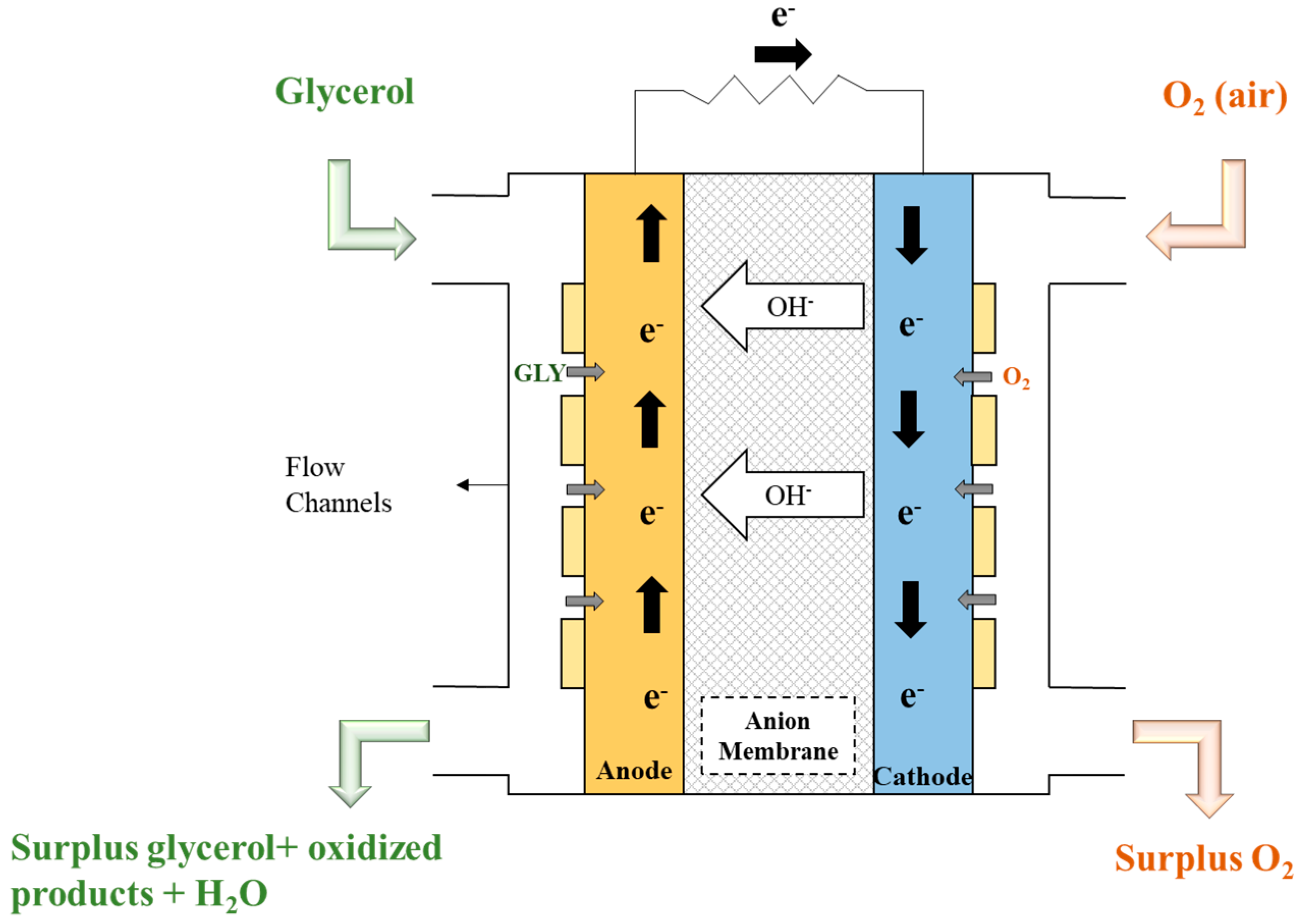
Figure 1. Schematic illustration of an SAMFC operating with glycerol.
Energies 16 06762 g001
Figure 2. Reaction scheme for the oxidation of glycerol in alkaline medium using a Pt electrode, based on Equations (6)–(17), employed in the present work.
Energies 16 06762 g002
Figure 3. Detailed structure of an artificial neural network.
Energies 16 06762 g003
Figure 4. PM polarization curve for the Pt/C electrode at 60 °C.
Energies 16 06762 g004
Figure 5. PM coverage fraction distribution for the Pt/C electrode at 60 °C.
Energies 16 06762 g005
Figure 6. Parameter sensitivity of the kinetic constants multiplied by (A) 1.1, (B) 1.5, and (C) 1.8.
Energies 16 06762 g006
Figure 7. Parametric sensitivity analysis of the transfer coefficients multiplied by (A) 1.05 and (B) 1.1 for the PM using the Pt/C electrode at 60 °C.
Energies 16 06762 g007
Figure 8. Effect of increasing the most sensitive kinetic constants (k2, k5, and k5′): (A) Original model, (B) 1.5-fold increase, (C) 5-fold increase, and (D) 10-fold increase.
Energies 16 06762 g008
Figure 9. Polarization curve for SPM2, performed with the Pt/C electrode and temperature of 60 °C.
Energies 16 06762 g009
Figure 10. Coverage fraction distribution for SPM2, performed with the Pt/C electrode and temperature of 60 °C.
Energies 16 06762 g010
Figure 11. Polarization curve for the phenomenological model with the Pt/C electrode at 90 °C.
Energies 16 06762 g011
Figure 12. Coverage fraction distribution for the PM with the Pt/C electrode at 90 °C.
Energies 16 06762 g012
Figure 13. Additional information about validation.
Energies 16 06762 g013
Figure 14. Regressions between the model output and the experimental values (targets) for the ANN with the PtAg/C and PtAg/MnOx/C electrodes at temperatures of 60 °C and 90 °C for (A) training, (B) validation, (C) testing, and (D) with all the sample data.
Energies 16 06762 g014
Figure 15. Responses of the ANN for the PtAg/C and PtAg/MnOx/C electrodes at temperatures of 60 °C and 90 °C.
Energies 16 06762 g015
Figure 16. Performance graphs for the ANN with the PtAg/C and PtAg/MnOx/C electrodes at temperatures of 60 °C and 90 °C: (A) performance of the ANN during the iterations; (B) histogram of errors for the ANN training, validation, and testing steps.
Energies 16 06762 g016
Table 1. Constants used in the model.
ConstantValueReference
R (V·C/(mol·K))8.314-
F (C/mol)96,485.3-
CGLY (mol/m3)1000[27]
CO2/CO2,ref1[27]
i0_c (A/m2)0.31[27]
Rmem (Ω·m2)2.85 × 10⁻⁵[23]
αC0.66Assumed
ilim 60 °C (A/m2)1400Assumed
ilim 90 °C (A/m2)3100Assumed
E0 (V)1.05Fitted to the ideal model
Table 2. Fitted values and SE, SD, and deviation magnitude for the most significant kinetic parameters of the phenomenological model for the Pt/C electrode at 60 °C.
ParameterUnitsValueSESDDeviation Magnitude
k2mol/(m2·s)1.65 × 10−37.47 × 10−61.53 × 10−59.24 × 10−3
k5mol/(m2·s)2.00 × 10−47.64 × 10−91.56 × 10−87.80 × 10−5
k5mol/(m2·s)1.001.05 × 10−22.14 × 10−22.14 × 10−2
α2-0.267.84 × 10−41.60 × 10−36.16 × 10−3
α4-1.503.05 × 10−66.23 × 10−64.16 × 10−6
Table 3. Fitted values and SE, SD, and deviation magnitude for SPM1 at 60 °C.
ParameterUnitsValueSESDDeviation Magnitude
k2mol/(m2·s)1.65 × 10−31.52 × 10−103.10 × 10−101.88 × 10⁻⁷
k5mol/(m2·s)2.00 × 10−41.05 × 10−112.14 × 10−111.07 × 10⁻⁷
k5mol/(m2·s)1.001.40 × 10−72.86 × 10−72.86 × 10−7
α2-0.263.53 × 10−97.20 × 10−92.77 × 10−8
α4-1.494.17 × 10−98.52 × 10−95.72 × 10−9
Table 4. Fitted values and SE, SD, and deviation magnitude for SPM2 at 60 °C.
ParameterUnitsValueSESDDeviation Magnitude
k2mol/(m2·s)1.65 × 10−31.46 × 10−82.97 × 10−81.80 × 10−5
k2mol/(m2·s)3.88 × 10−23.56 × 10−77.27 × 10−71.87 × 10−5
k5mol/(m2·s)2.00 × 10−44.89 × 10−121.00 × 10−125.00 × 10⁻⁸
k5mol/(m2·s)0.256.14 × 10−41.25 × 10−45.03 × 10−3
α2-0.261.76 × 10−83.59 × 10−81.38 × 10−7
α4-1.542.35 × 10−94.79 × 10−93.11 × 10−9
Table 5. Comparison of the fitted values and the relative deviations of the most sensitive kinetic parameters, for the full PM, SPM1, and SPM2.
Full PMSPM1SPM2
ParameterValueDeviation MagnitudeValueDeviation MagnitudeValueDeviation Magnitude
k21.65 × 10−39.24 × 10−31.65 × 10−31.88 × 10−71.65 × 10−31.80 × 10⁻⁵
k52.00 × 10−47.80 × 10−52.00 × 10−41.07 × 10−72.00 × 10−45.00 × 10⁻⁸
k51.002.14 × 10−21.002.86 × 10−70.255.03 × 10−3
α20.266.16 × 10−30.262.77 × 10−80.261.38 × 10−7
α41.504.16 × 10−61.495.72 × 10−91.543.11 × 10−9
Table 6. Fitted values, SE, SD, and deviation magnitude for the phenomenological model with the Pt/C electrode at 90 °C.
ParameterUnitsValueSESDDeviation Magnitude
k2mol/(m2·s)4.50 × 10−31.15 × 10−62.35 × 10−65.23 × 10−4
k5mol/(m2·s)2.00 × 10−41.53 × 10−103.12 × 10−101.56 × 10⁻⁶
k5mol/(m2·s)1.00 × 10−23.56 × 10−67.27 × 10−67.25 × 10−4
α2-0.401.89 × 10−53.85 × 10−59.64 × 10−5
α4-1.751.65 × 10−73.38 × 10−71.93 × 10−7
Table 7. Literature and pros and cons of the phenomenological models.
Phenomenological Models
Literature
  • Demirel et al. [35] performed an investigation of oxidation using an alkaline DGFC with a gold electrode supported on carbon (Au/C). The proposed mechanistic kinetic model was based on the Langmuir–Hinshelwood mechanism, considering that there was no mass transfer limitation. The model parameters were calculated via nonlinear regression. The main parameters studied were the activation energies, reaction orders, adsorption constants, and kinetic constants. The standard errors for these parameters were also calculated together with the relative standard errors. The most relevant adsorbed products found were glyceric acid and tartronic acid in addition to the glycerol fuel.
  • A work by Han et al. [27] described the unidimensional mechanistic modeling of a DGFC with anion exchange membrane and Au/C catalyst, operating under steady-state and dynamic conditions. The only major product of the reaction considered was tartronic acid, and the kinetic model was based on the Butler–Volmer equations. In addition to kinetic equations, mass transport and cell voltage equations were also used. The numerical simulation for the steady-state regime employed polarization and power curves, together with the absolute anodic and cathodic overpotential values. The simulated curves were able to accurately describe the experimental data. The model also included estimates of the anodic, cathodic, and ohmic voltage losses.
This Work:
Pros
  • The phenomenological model proposed can describe very well the mechanism and the experimental data in all cases evaluated (PM at 60 °C, SPMs 1 and 2, and PM at 90 °C).
  • The statistical study of the model kinetic parameters provides essential information concerning the specific parameters that significantly influence the behavior of the polarization curve. The parametrical sensitivity (graphical method) confirmed the high influence of the most significant kinetic parameters found in the statistical study, which demonstrates how solid and robust the approach is.
  • The interdependence between the model parameters (specially the most sensitive kinetic parameters) and the degree of coverage of the catalyst can enable evaluation of possible changes in the amount of a particular product actually obtained.
  • Versatility of the model, where simplified models can be obtained from the general model. Also, it is possible to incorporate additional intermediates and products into the reaction mechanism.
This Work:
Cons
  • The phenomenological modeling process can become very complex for bimetallic electrodes, so it would be currently unfeasible to develop complete mechanistic models capable of accurately describing all the mechanisms involved in these cases.
Table 8. Literature and pros and cons of the artificial neural networks.
Artificial Neural Networks
LiteratureThere is no literature concerning ANNs applied to alkaline DGFCs.
This Work:
Pros
  • This work fills a gap in the literature regarding the application of ANNs to an alkaline DGFC.
  • ANNs enable representation (with high prediction accuracy) of the functional interdependence between input variables and cell current density, which can be convenient in cases that are too complex for the application of a complete mechanistic modeling.
This Work:
Cons
  • This approach (black box model) cannot describe any aspects of the mechanism involved (physical, chemical, electrochemical, thermal, etc.), which means that no insights about the process can be extracted from this type of model.
Disclaimer/Publisher’s Note: The statements, opinions and data contained in all publications are solely those of the individual author(s) and contributor(s) and not of MDPI and/or the editor(s). MDPI and/or the editor(s) disclaim responsibility for any injury to people or property resulting from any ideas, methods, instructions or products referred to in the content.