Computation of High-Order Sensitivities of Model Responses to Model Parameters—I: Underlying Motivation and Current Methods

Abstract

The mathematical/computational model of a physical system comprises parameters and independent and dependent variables. Since the physical system is seldom known precisely and since the model’s parameters stem from experimental procedures that are also subject to uncertainties, the results predicted by a computational model are imperfect. Quantifying the reliability and accuracy of results produced by a model (called “model responses”) requires the availability of sensitivities (i.e., functional partial derivatives) of model responses with respect to model parameters. This work reviews the basic motivations for computing high-order sensitivities and illustrates their importance by means of an OECD/NEA reactor physics benchmark, which is representative of a “large-scale system” involving many (21,976) uncertain parameters. The computation of higher-order sensitivities by conventional methods (finite differences and/or statistical procedures) is subject to the “curse of dimensionality”. Furthermore, as will be illustrated in this work, the accuracy of high-order sensitivities computed using such conventional methods cannot be a priori guaranteed. High-order sensitivities can be computed accurately and efficiently solely by applying the high-order adjoint sensitivity analysis methodology. The principles underlying this adjoint methodology are also reviewed in preparation for introducing, in the accompanying Part II, the “High-Order Function/Feature Adjoint Sensitivity Analysis Methodology” (nth-FASAM), which aims at most efficiently computing exact expressions of high-order sensitivities of model responses to functions (“features”) of model parameters.

1. Introduction

The mathematical/computational models of physical systems comprise parameters and independent and dependent variables. The system’s independent variables and parameters are related to the system’s state (i.e., dependent) through a well-posed system of equations, which is usually nonlinear in all of its components. The minimum amount of information needed to use a model is the availability of nominal or mean values for the system parameters. With the known nominal parameter values, a model can be used to compute results of interest, which are called model/system “responses”, “objective functions”, or “indices of performance”. Since the physical processes themselves are seldom known precisely and since most of the model’s parameters stem from experimental procedures that are also subject to imprecisions and/or uncertainties, the results predicted by these models are also imprecise, being affected by the uncertainties underlying the respective model. Quantifying the reliability and accuracy of results (responses) computed using models is achieved by performing activities known as “sensitivity analysis”, “uncertainty quantification”, “model verification”, “model validation”, “data assimilation”, “model calibration”, and “predictive modeling”. Sensitivity analysis aims at quantifying the changes in the computed response that would be induced by changes in the model parameters, along with understanding the model by ranking the importance of the various parameters in contributing to the response. The availability of such rankings makes it possible to prioritize improvements in the model and also streamline it by eliminating unimportant parameters and/or processes to develop “reduced-order models”. Uncertainty quantification aims at quantitatively determining the uncertainties induced in a model response due to model parameter uncertainties. Model verification deals with the question, “Are the equations underlying the model solved correctly?” Model validation compares the model’s computational results to experimental information in order to address the question, “Does the model represent reality?” Data assimilation combines experimental and computational information to improve model responses while model calibration uses experimental information to adjust/calibrate the parameters to improve the accuracy of future computations. “Predictive modeling” aims at obtaining “best-estimate” optimally predicted results with reduced predicted uncertainties, subsuming data assimilation and model calibration. All of these activities, as well as optimizing the system and using models for “inverse problems”, require the availability of the functional derivatives—called “sensitivities”—of model responses with respect to the imprecisely known model parameters.

For large-scale models involving many parameters, even the first-order sensitivities are very expensive to compute by conventional methods. It is known that the “adjoint method” of sensitivity analysis is the most efficient method for computing exactly first-order sensitivities since it requires a single large-scale (adjoint) computation, independently of the number of model parameters. Cacuci [1,2] has conceived the rigorous first-order adjoint sensitivity analysis methodology for generic large-scale nonlinear (as opposed to linearized) systems involving generic operator responses and for having introduced these principles to the earth, atmospheric and other sciences, as credited, e.g., by Práger and Kelemen [3] and Luo, Wang, and Liu [4].

The computation of higher-order sensitivities by conventional methods is subject to the “curse of dimensionality”, a term coined by Bellman [5] to describe phenomena in which the number of computations increases exponentially in the respective phase space. In the particular case of sensitivity analysis using conventional methods, the number of large-scale computations increases exponentially in the phase space of the model parameter as the order of sensitivities increases. The general mathematical framework for the second-order adjoint sensitivity analysis methodology for generic linear and nonlinear systems, respectively, was conceived by Cacuci [6,7,8]. The unparalleled efficiency of the second-order adjoint sensitivity analysis methodology for linear systems was demonstrated [9,10,11,12,13,14] by applying this methodology to compute exactly the 21,976 first-order sensitivities and 482,944,576 second-order sensitivities (of which 241,483,276 are distinct from each other) for an OECD/NEA reactor physics benchmark [15], which is representative of a large-scale system that involves many (21,976, in this illustrative example) parameters. Such a large-scale system cannot be analyzed exactly and comprehensively by any other methods. Contrary to the widely held belief that second- and higher-order sensitivities are negligible for reactor physics systems, it was found [9,10,11,12,13,14] that many second-order sensitivities of the OECD benchmark’s response to the benchmark’s uncertain parameters were much larger than the largest first-order ones. This finding has motivated the investigation of the largest third-order sensitivities, many of which were found [16,17] to be even larger than the second-order ones. This finding has motivated the development of the mathematical framework for determining and computing the fourth-order sensitivities [18], many of which were found to be larger than the third-order ones. This sequence of findings has motivated the conception by Cacuci [19] of the nth-Order Comprehensive Adjoint Sensitivity Analysis Methodology for Response-Coupled Forward/Adjoint Linear Systems (abbreviated as “nth-CASAM-L”). The nth-CASAM-L overcomes the curse of dimensionality in sensitivity analysis, enabling the efficient computation of exactly determined expressions of arbitrarily high-order sensitivities of a generic system response—which can depend on both the forward and adjoint state functions for linear systems—with respect to all of the parameters that characterize the physical system. The “nth-CASAM-L” mathematical framework was developed specifically for linear systems because the most important model responses produced by such systems are various Lagrangian functionals, which depend simultaneously on both the forward and adjoint state functions governing the respective linear system. Such responses can occur only for linear systems because responses in nonlinear systems can only depend on the system’s forward state functions (since nonlinear operators do not admit adjoint operators).

In parallel with the aforementioned developments, Cacuci [20] has extended his original work [1,2] on nonlinear systems to include the treatment of uncertain boundaries and interfaces, encompassing the mathematical framework for deriving and computing efficiently the exact expressions of sensitivities up to and including the fifth-order. This general methodology is called the nth-Order Comprehensive Adjoint Sensitivity Analysis Methodology for Nonlinear Systems (abbreviated as nth-CASAM-N). Similar to the nth-CASAM-L, the nth-CASAM-N [19] is formulated in linearly increasing higher-dimensional Hilbert spaces (as opposed to exponentially increasing parameter-dimensional spaces), thus overcoming the curse of dimensionality in sensitivity analysis of nonlinear systems, enabling the most efficient computation of exactly determined expressions of arbitrarily high-order sensitivities of generic nonlinear system responses with respect to model parameters, uncertain boundaries, and internal interfaces in the model’s phase space. Additional details regarding applications of the nth-CASAM-L and the nth-CASAM-N methodologies are provided in [21,22,23].

This work is structured as follows: Section 2 presents the mathematical modeling of physical systems, which comprises imprecisely known (uncertain) model parameters and physical boundaries that could arise from manufacturing tolerances. Using the OECD/NEA reactor physics benchmark [15], Section 3 illustrates the essential role and impact of high-order sensitivities in uncertainty quantification and predictive modeling. Section 4 illustrates the difficulties involved in computing high-order sensitivities using finite difference formulas, which, along with the high-order adjoint sensitivity analysis methodologies, nth-CASAM-N and nth-CASAM-N, are the only procedures available for computing high-order sensitivities. Section 4 also reviews the principles underlying the nth-CASAM-N, which will be used in the accompanying Part II [24] to conceive the “High-Order Function/Feature Adjoint Sensitivity Analysis Methodology” (nth-FASAM), which aims at computing exact expressions of high-order sensitivities of model responses to functions (“features”) of model parameters, which actually are found in many models in practice. By means of an illustrative paradigm example of particle transport (i.e., a simplified version of the OECD/NEA reactor physics benchmark [14]), the accompanying Part II [24] highlights the unparalleled gain in efficiency of the nth-FASAM (to be developed in [24]) by comparison to the nth-CASAM, which itself is currently peerless in terms of accuracy and efficiency for computing high-order sensitivities of responses to model parameters.

2. Modeling of a Nonlinear Physical System Comprising Imprecisely Known Parameters and Boundaries

The mathematical model that underlies the numerical evaluation of a process and/or state of a physical system comprises equations that relate the system’s independent variables and parameters to the system’s state/dependent variables. Such a model can generically be modeled by means of coupled equations, which are in general nonlinear, and can be represented in operator form as follows:

$$N\left[u\left(x\right);x;\alpha \right]=Q\left(x;\alpha \right),\hspace{1em}x\in {\mathsf{\Omega }}_x\left(x\right);$$

(1)

$$B\left[u\left(x\right);\alpha \right]=C\left(\alpha \right),\hspace{1em}x\in \partial {\mathsf{\Omega }}_x\left(\alpha \right).$$

(2)

Matrices are denoted using capital bold letters, while vectors are denoted using either capital or lower-case bold letters. The symbol “$\triangleq$” is used to denote “is defined as” or “is by definition equal to”. Transposition is indicated by a dagger $(†)$ superscript. The equalities in this work are considered to hold in the weak (“distributional”) sense. The right sides of Equations (1) and (2), as well as other equations to be derived in this work, may contain “generalized functions/functionals”, particularly Dirac distributions and derivatives thereof.

The results computed using a mathematical model are customarily called “model responses” (or “system responses”, “objective functions”, or “indices of performance”). As has been discussed in [21,23], all responses can be fundamentally analyzed in terms of the following generic integral representation:

$$R\left[u\left(x\right);\alpha \right]\triangleq {\displaystyle \underset{{\lambda }_1\left(\alpha \right)}{\overset{{\omega }_1\left(\alpha \right)}{\int }}\dots {\displaystyle \underset{{\lambda }_{TI}\left(\alpha \right)}{\overset{{\omega }_{TI}\left(\alpha \right)}{\int }}S\left[u\left(x\right);x;\alpha \right]d{x}_1\dots d{x}_{TI}}},$$

(3)

where $S\left[u\left(x\right);x;\alpha \right]$ is a suitably differentiable nonlinear function of $u\left(x\right)$ and of $\alpha$.

Without loss of generality, the quantities that appear in Equations (1)–(3) can be considered to be real-valued and have the following meanings:

1. The column-vector $\alpha \triangleq {\left({\alpha }_1,\dots ,{\alpha }_{TP}\right)}^{†}\in {ℝ}^{TP}$ represents the “vector of primary model parameters” and has components denoted as ${\alpha }_1$, …, ${\alpha }_{TP}$, where $TP$ denotes the “total number of parameters” underlying the model under consideration. These parameters are “input” for the model and are subject to uncertainties stemming from processes that are external to the system under consideration. The nominal (expected/mean) values of the model parameters are considered to be known and will be denoted as ${\alpha }^0\triangleq {\left({\alpha }_1^0,\dots ,{\alpha }_i^0,\dots ,{\alpha }_{TP}^0\right)}^{†}$; the superscript “0” will be used throughout this monograph to denote “nominal values”. The components of the vector $\alpha$ include not only parameters that appear in Equations (1) and (2), which define the computational model but also include parameters that may specifically occur only in the definition of the model’s response under consideration, cf. Equation (3). Without loss of generality, the model parameters ${\alpha }_1$, …, ${\alpha }_{TP}$ can be considered for real-valued scalars;

2. The column vector $x\triangleq {\left(x_1,\dots ,x_{TI}\right)}^{†}\in {ℝ}^{TI}$ comprises the model’s independent variables, denoted as $x_i,i=1,\dots ,TI$, where “TI” denotes the “total number of independent variables”. The vector $x\in {ℝ}^{TI}$ is considered to be defined on a phase space domain denoted as ${\mathsf{\Omega }}_x\left(x\right)\triangleq \left\{{\lambda }_i\left(\alpha \right)\le x_i\le {\omega }_i\left(\alpha \right);i=1,\dots ,TI\right\}$; the particular cases when ${\lambda }_i\left(\alpha \right)=-\infty ,{\omega }_i\left(\alpha \right)=\infty$ for some independent variables $x_i,\hspace{1em}i=1,\dots ,TI$ are included. The domain boundary $\partial {\mathsf{\Omega }}_x\left[\lambda \left(\alpha \right);\omega \left(\alpha \right)\right]\triangleq \left\{{\lambda }_i\left(\alpha \right)\cup {\omega }_i\left(\alpha \right),\hspace{1em}i=1,\dots ,TI\right\}$ of ${\mathsf{\Omega }}_x\left(x\right)$ is defined to comprise the set of all of the endpoints ${\lambda }_i\left(\alpha \right),\hspace{1em}{\omega }_i\left(\alpha \right),\hspace{1em}i=1,\dots ,TI$. These endpoints depend on the physical system’s geometrical dimensions, which may be imprecisely known because of manufacturing tolerances, and are considered, therefore, to be components of the vector $\alpha \triangleq {\left({\alpha }_1,\dots ,{\alpha }_{TP}\right)}^{†}\in {ℝ}^{TP}$ of primary model parameters. Furthermore, the boundary endpoints, ${\lambda }_i\left(\alpha \right),\hspace{1em}{\omega }_i\left(\alpha \right),\hspace{1em}i=1,\dots ,TI$, may also depend on the parameters that define the material properties of the respective medium. For example, in models based on diffusion theory, the boundary conditions for materials facing air/vacuum are imposed on the “extrapolated boundary” of the respective spatial domain. The “extrapolated boundary” depends both on the imprecisely known physical dimensions of the system’s materials and also on the material’s properties, such as atomic number densities and microscopic transport cross-sections;

3. The column vector $u\left(x\right)\triangleq {\left[u_1\left(x\right),\dots ,u_{TD}\left(x\right)\right]}^{†}$ comprises the model’s dependent variables $u_i\left(x\right),i=1,\dots ,TD$; the abbreviation “$TD$” denotes the “total number of dependent variables”;

4. The column vector $N\left[u\left(x\right);x;\alpha \right]\triangleq {\left(N_1,\dots ,N_{TD}\right)}^{†}$ comprises components $N_i\left[u\left(x\right);x;g\left(\alpha \right)\right],i=1,\dots ,TD$, which are operators that act linearly and/or nonlinearly on $u\left(x\right)$, $x$, and $\alpha$;

5. The components $q_i\left[u\left(x\right);x;\alpha \right],i=1,\dots ,TD$ of the $TD$-dimensional column vector $Q\left[u\left(x\right);x;\alpha \right]\triangleq {\left(q_1,\dots ,q_{TD}\right)}^{†}$ denote inhomogeneous source terms;

6. The components of $B\left[u\left(x\right);\alpha ;x\right]$ and $C\left(\alpha \right)$ are nonlinear operators that represent boundary and/or initial conditions on $\partial {\mathsf{\Omega }}_x$.

3. Motivation for Computing Exact Expressions of High-Order Response Sensitivities to Parameters

Historically, the concept of “sensitivity analysis” arose from the need to predict and quantify the changes induced in the model’s responses by changes in the model parameters and to rank the importance of the model’s parameters in affecting the model’s responses. Initially, such predictions were performed by simply recomputing the result of interest using the variations of interest in the model parameters. Evidently, the results provided by such re-computations are specific to the respective parameter variation. Furthermore, such re-computations become unfeasible for large-scale models with many parameters. Nevertheless, such re-computations had become the basis for computing approximately, using finite differences, various partial derivatives of the response with respect to model parameters, which played the role of “sensitivities of responses with respect to parameters”. Subsequently, statisticians introduced various quantities (e.g., “measures of sensitivities” and/or “sensitivity indicators”) to play the role of “sensitivities” by using statistical quantities related to the variance of the response that might be induced by the variances assumed to be known, of the model parameters. These statistical measures and methodologies to compute them will also be mentioned briefly in this Section.

Mathematically, the only unambiguous concept for defining the “sensitivity of a function to its underlying parameters” is in terms of the partial derivatives of the respective function with respect to its underlying parameters. Thus, the “first-order sensitivities” of a model response are the first-order partial functional derivatives of the response with respect to the parameters; the “second-order sensitivities” are the second-order partial functional derivatives of the response with respect to the parameters; and so on; the “nth-order sensitivities” are the nth-order partial functional derivatives of the model response with respect to the model parameters.

There are three major areas of scientific activities that are built on the availability of response sensitivities to model parameters as follows: (i) sensitivity analysis; (ii) uncertainty quantification; and (iii) predictive modeling, which combines measured and computational information to obtain best-estimate predictions of model responses and parameters, with reduced predicted uncertainties. The current state-of-the-art in these three areas of scientific activities will be reviewed briefly in this Section.

3.1. High-Order Sensitivity Analysis

The scope of “sensitivity analysis” is to predict and quantify the changes induced in the model’s response by changes in the model parameters and to rank the importance of the model’s parameters in affecting the model’s response. Mathematically, the soundest concept for predicting unambiguously the changes induced in a function of parameters stemming from changes in the respective parameters is provided by the multivariate Taylor series of the function with respect to its component parameters. Hence, the concept of “sensitivity of a function to its underlying parameters” is based on the role of the partial derivatives of the respective function with respect to its underlying parameters. Specifically, the “first-order sensitivities” of a model response are the first-order partial functional derivatives of the response with respect to the parameters; the “second-order sensitivities” are the second-order partial functional derivatives of the response with respect to the parameters; and so on; the “nth-order sensitivities” are the nth-order partial functional derivatives of the model response with respect to the model parameters. Since the expected (or nominal) parameter values, ${\alpha }^0$, are known, the formal expression of the multivariate Taylor series expansion of a model response, denoted as $R_k\left(\alpha \right)$, as a function of the model parameters $\alpha \triangleq {\left({\alpha }_1,\dots ,{\alpha }_{TP}\right)}^{†}\in {ℝ}^{TP}$ around ${\alpha }^0$ has the following well-known formal expression:

$$\begin{array}{l}{R}_k\left(\alpha \right)=R_k\left({\alpha }^0\right)+{\displaystyle \sum _{j_1=1}^{TP}{\left\{\frac{\partial R_k\left(\alpha \right)}{\partial {\alpha }_{j_1}}\right\}}_{{\alpha }^0}\delta {\alpha }_{j_1}}+\frac{1}{2}{\displaystyle \sum _{j_1=1}^{TP}{\displaystyle \sum _{j_2=1}^{TP}{\left\{\frac{{\partial }^2{R}_k\left(\alpha \right)}{\partial {\alpha }_{j_1}\partial {\alpha }_{j_2}}\right\}}_{{\alpha }^0}}}\delta {\alpha }_{j_1}\delta {\alpha }_{j_2}\\ \hspace{1em}\hspace{1em}+\frac{1}{3!}{\displaystyle \sum _{j_1=1}^{TP}{\displaystyle \sum _{j_2=1}^{TP}{\displaystyle \sum _{j_3=1}^{TP}{\left\{\frac{{\partial }^3{R}_k\left(\alpha \right)}{\partial {\alpha }_{j_1}\partial {\alpha }_{j_2}\partial {\alpha }_{j_3}}\right\}}_{{\alpha }^0}}}}\delta {\alpha }_{j_1}\delta {\alpha }_{j_2}\delta {\alpha }_{j_3}\\ \hspace{1em}\hspace{1em}+\frac{1}{4!}{\displaystyle \sum _{j_1=1}^{TP}{\displaystyle \sum _{j_2=1}^{TP}{\displaystyle \sum _{j_3=1}^{TP}{\displaystyle \sum _{j_4=1}^{TP}{\left\{\frac{{\partial }^4{R}_k\left(\alpha \right)}{\partial {\alpha }_{j_1}\partial {\alpha }_{j_2}\partial {\alpha }_{j_3}\partial {\alpha }_{j_4}}\right\}}_{{\alpha }^0}}}}}\delta {\alpha }_{j_1}\delta {\alpha }_{j_2}\delta {\alpha }_{j_3}\delta {\alpha }_{j_4}+\dots ,\end{array}$$

(4)

where $\delta {\alpha }_j\triangleq \left({\alpha }_j-{\alpha }_j^0\right),j=1,\dots ,TP$. Since the explicit expression of $R_k\left(\alpha \right)$ as a function of the model parameters $\alpha \triangleq {\left({\alpha }_1,\dots ,{\alpha }_{TP}\right)}^{†}\in {ℝ}^{TP}$ is not available, the explicit expressions of the sensitivities of $R_k\left(\alpha \right)$ are not available for numerical evaluation. It is evident from Equation (4) that, for a model comprising a total number of $TP$-parameters, for each model response, there are $TP$ first-order sensitivities, $TP\left(TP+1\right)/2$ distinct second-order sensitivities, $TP\left(TP+1\right)\left(TP+2\right)/6$ distinct third-order sensitivities, and so on. The number of sensitivities increases exponentially with the order of the respective sensitivities; hence, their computation by conventional methods (e.g., finite difference schemes, statistical assessments), which require re-computations using the original model (with suitably altered parameter values) is hampered by the curse of dimensionality [5] while providing approximate (often inaccurate), rather than exact, values for the sensitivities. The only extant method that overcomes, to the largest possible extent, the curse of dimensionality while providing exact expressions for computing efficiently sensitivities of all orders is the “nth-Order Comprehensive Adjoint Sensitivity Analysis Methodology (nth-CASAM)” developed by Cacuci [21,23] by extending the original adjoint sensitivity analysis methodology conceived by Cacuci [1,2]. The nth-CASAM requires computations in linearly increasing higher-dimensional Hilbert spaces, as opposed to exponentially increasing parameter-dimensional spaces. In particular, for a scalar-valued response associated with a model comprising $TP$ model parameters, the nth-CASAM requires one adjoint computation for computing exactly all of the first-order response sensitivities, as opposed to at least $TP$ forward computations, as required by other methods to obtain approximate values for these sensitivities. All of the (mixed) second-order sensitivities are computed exactly by the nth-CASAM in most $TP$ computations, as opposed to needing at least $TP\left(TP+1\right)/2$ computations, as required by all other methods, and so on. For every lower-order sensitivity of interest, the nth-CASAM computes the “$TP$ next-higher-order” sensitivities in one adjoint computation performed in a linearly increasing higher-dimensional Hilbert space. The nth-CASAM applies to any model (deterministic, statistical, etc.) and is also applicable to the computation of sensitivities of operator-valued responses, which cannot be obtained by statistical methods when the underlying problem comprises many parameters. The larger the number of model parameters, the more efficient the nth-CASAM becomes for computing arbitrarily high-order response sensitivities.

The practitioners of statistical methods cavalierly downplay the importance of the Taylor series by labeling it as being “local” (as opposed to “global”—as they usually characterize the statistical methods). In reality, the range of validity of the Taylor series is provided by its radius of convergence. The accuracy—as opposed to the “validity”—of the Taylor series in predicting the value of the response at an arbitrary point in the phase space of model parameters depends on the order of sensitivities retained in the Taylor expansion: the higher the respective order, the more accurate the respective response value predicted by the Taylor series. In the particular cases when the response happens to be a polynomial function of the model parameters, the Taylor series is actually exact (not only “non-local”). In contradistinction, no statistical method is ever “exact.

The need for the computation of higher-order sensitivities has been amply illustrated by Cacuci and Fang [22], using as a paradigm model the polyethylene-reflected plutonium (acronym “PERP”) reactor physics benchmark [15], which is included in the Nuclear Energy Agency (NEA) International Criticality Safety Benchmark Evaluation Project (ICSBEP). The composition and dimensions of this benchmark are summarized in Appendix A. The distribution of neutrons within the benchmark is modeled by the linear time-independent inhomogeneous neutron transport (Boltzmann) equation (see Appendix A), which is solved numerically (after discretization in the energy, spatial, and angular independent variables) using the software package PARTISN [25] and SOURCES4C [26]. The numerical model of the PERP benchmark includes 21,976 parameters, of which the following 7477 parameters have non-zero (but imprecisely known) nominal values: 180 group-averaged total microscopic cross-sections; 120 fission process parameters; 60 fission spectrum parameters; 10 parameters describing the experiment’s nuclear sources; 6 isotopic number densities; and 7101 non-zero group-averaged scattering microscopic cross-sections (the remaining scattering cross-sections, out of a total of 21,600, have zero nominal values). Solving the Boltzmann equation with these many parameters is representative of a “large-scale computation”.

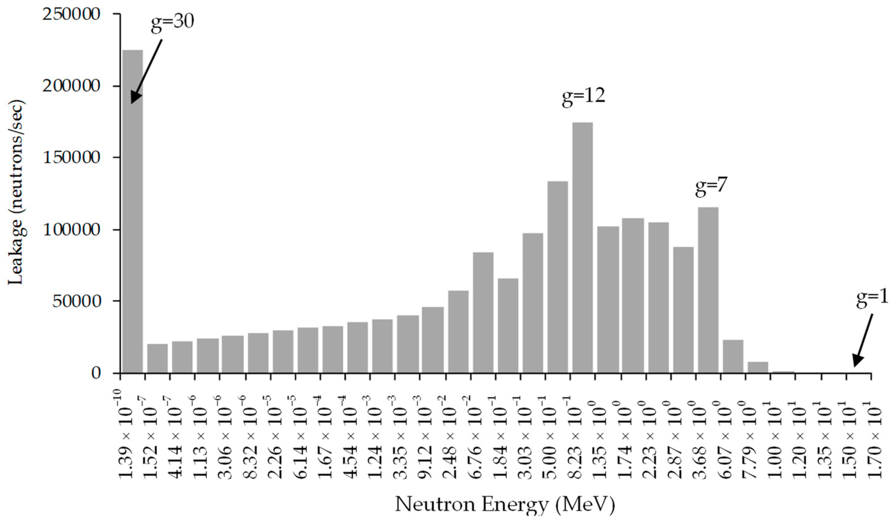
The response of interest for the PERP benchmark is the total neutron leakage from the PERP sphere (numerical value: $1.7648\times {10}^6$ neutrons/s), which is plotted in histogram form as a function of energy in Figure 1 [22].

All of the first-order sensitivities of the leakage response with respect to the 7477 non-zero parameters were computed [22] using the First-Order Comprehensive Sensitivity Analysis Methodology (first-CASAM). The vast majority of these sensitivities had relative values below 10%, but 16 of them exceeded unity in absolute value; the largest of all of the first-order relative sensitivities was the sensitivity of the leakage response with respect to the total group cross-section, denoted as ${\sigma }_{t,6}^{30}$, of Hydrogen (labeled isotope #6) in group 30, which had the relative value $S^{(1)}\left({\sigma }_{t,6}^{30}\right)=-9.366$. Among the benchmark’s parameters, the total microscopic cross-sections had the largest impact on the leakage response; the following sensitivities of this response with respect to the microscopic total cross-sections of hydrogen also had large values for energy groups 17–20 [$S^{(1)}\left({\sigma }_{t,i=6}^{16}\right)=-1.164$; $S^{(1)}\left({\sigma }_{t,i=6}^{17}\right)=-1.173$; $S^{(1)}\left({\sigma }_{t,i=6}^{18}\right)=-1.141$; $S^{(1)}\left({\sigma }_{t,i=6}^{19}\right)=-1.094$; $S^{(1)}\left({\sigma }_{t,i=6}^{20}\right)=-1.033$). Also included in the top 16 were the (relative) sensitivities of the leakage response with respect to the total microscopic cross-sections of ²³⁹Pu (labeled isotope #1) in energy groups 12 and 13, which had the values $S^{(1)}\left({\sigma }_{t,i=1}^{12}\right)=-1.320$ and $S^{(1)}\left({\sigma }_{t,i=1}^{13}\right)=-1.154$, respectively.

The second-order sensitivities also must be computed in order to compare them with the values of the largest first-order sensitivities and consequently decide which, if any, of the second-order sensitivities must be retained for subsequent uses (e.g., for uncertainty quantification and/or data assimilation and predictive modeling). Therefore, all of the distinct (7477 × 7478/2) second-order sensitivities of the PERP benchmark’s leakage response with respect to the benchmark’s parameters were computed [9,10,11,12,13,14,22] by applying the Second-Order Comprehensive Sensitivity Analysis Methodology (second-CASAM). It was thus established that ca. 1000 relative second-order sensitivities had absolute values larger than unity, with over 50 of them having absolute values between 10.0 and 100.0. The overall largest second-order relative sensitivity was the unmixed second-order sensitivity of the leakage response with respect to the total microscopic cross-section of hydrogen in energy group 30, which had the value $S^{(2)}\left({\sigma }_{t,6}^{30},{\sigma }_{t,6}^{30}\right)=429.6$.

These findings have motivated the computation [16,17,22] of the third-order sensitivities of the leakage response with respect to the benchmark’s total cross-sections. It was found there that 45,970 of such third-order sensitivities had absolute values between 1.0 and 10.0; 11,861 of such third-order sensitivities had absolute values between 10.0 and 100.0, and 1199 of such third-order sensitivities had absolute values larger than 100.0. All of the largest first-, second-, and third-order sensitivities involved the microscopic total cross-section for the lowest (30th) energy group of isotope ¹H (i.e., ${\sigma }_{t,6}^{30}$). The largest overall third-order sensitivity is the mixed third-order sensitivity $S^{(3)}\left({\sigma }_{t,1}^{g=30},{\sigma }_{t,6}^{g^{\prime }=30},{\sigma }_{t,6}^{g^{″}=30}\right)=-1.88\times {10}^5$, which also involves the microscopic total cross-section for the 30th energy group of isotope ²³⁹Pu (i.e., ${\sigma }_{t,1}^{g=30}$). The total microscopic cross-section of isotopes ¹H and ²³⁹Pu are the two most important parameters affecting the PERP benchmark’s leakage response since they are involved in all of the large second- and third-order sensitivities.

These results subsequently motivated the computation [18,19,22] of the fourth-order sensitivities of the leakage response with respect to the total microscopic cross-section of hydrogen. Depending on the specific energy group, the values of the fourth-order relative sensitivity were found to be ca. 2 to 7 times larger than the corresponding third-order ones, ca. 5 to 52 times larger than the values of the corresponding second-order sensitivities, and ca. 8 to 220 times larger than the values of the corresponding first-order sensitivities. For illustrative purposes, the energy-dependence of the first- through fourth-order sensitivities of the leakage response with respect to the total microscopic cross-sections of hydrogen are depicted in Figure 2 [22], which underscores the overwhelming importance of the second- and higher-order sensitivities.

3.2. High-Order Uncertainty Quantification

In practice, the model parameters are not known exactly, even though they are not bona fide random quantities. For practical purposes, however, these model parameters are considered to be variates that obey a multivariate probability distribution function, denoted as $p_{\alpha }\left(\alpha \right)$. Although this distribution is seldom known, the various moments of $p_{\alpha }\left(\alpha \right)$ can be defined in a standard manner by using the following notation for the “expected (or mean) value” of a function, $u\left(\alpha \right)$, of the parameters, which is defined over the domain of definition of $p_{\alpha }\left(\alpha \right)$:

$$E\left[u\left(\alpha \right)\right]\triangleq {\displaystyle \int u\left(\alpha \right)p_{\alpha }\left(\alpha \right)d\alpha },$$

(5)

In particular, the vector of expected values, ${\alpha }_j^0$, of the model parameters ${\alpha }_j$, is defined as follows:

$${\alpha }^0\triangleq {\left({\alpha }_1^0,\dots ,{\alpha }_{TP}^0\right)}^{†},\hspace{1em}\hspace{1em}{\alpha }_j^0\triangleq E\left({\alpha }_j\right),\hspace{1em}j=1,\dots ,TP.$$

(6)

In practice, the expected values—which are taken as the nominal values for carrying out the computation of responses using the mathematical/numerical model—are known (or assumed to be known). In order to perform “uncertainty quantification/analysis” of the uncertainties induced in the responses by uncertainties in the parameters, it is necessary to also know the covariances, $\mathrm{cov}\left({\alpha }_i,{\alpha }_j\right)$, between two parameters, ${\alpha }_i$ and ${\alpha }_j$, which are defined as follows:

$$\mathrm{cov}\left({\alpha }_i,{\alpha }_j\right)\triangleq E\left(\delta {\alpha }_i\delta {\alpha }_j\right)\triangleq {\rho }_{ij}{\sigma }_i{\sigma }_j,\hspace{1em}\hspace{1em}i,j=1,\dots ,TP.$$

(7)

In Equation (7), the quantities ${\sigma }_i$ and ${\sigma }_j$ denote the standard deviations of ${\alpha }_i$ and ${\alpha }_j$, respectively, while ${\rho }_{ij}$ denotes the correlation between the respective parameters. Occasionally, the higher-order correlations between parameters can also be obtained. Formally, the third-order correlation, $t_{j1j2j3}$, among three parameters is defined as follows:

$$t_{j_1{j}_2{j}_3}{\sigma }_{j_1}{\sigma }_{j_2}{\sigma }_{j_3}\triangleq E\left(\delta {\alpha }_{j_1}\delta {\alpha }_{j_2}\delta {\alpha }_{j_3}\right);\hspace{1em}\hspace{1em}{j}_1,j_2,j_3=1,\dots ,TP.$$

(8)

The fourth-order correlation $q_{j_1{j}_2{j}_3{j}_4}$ among four parameters is defined as follows:

$$q_{j_1{j}_2{j}_3{j}_4}{\sigma }_{j_1}{\sigma }_{j_2}{\sigma }_{j_3}{\sigma }_{j_4}\triangleq E\left(\delta {\alpha }_{j_1}\delta {\alpha }_{j_2}\delta {\alpha }_{j_3}\delta {\alpha }_{j_4}\right);\hspace{1em}{j}_1,j_2,j_3,j_4=1,\dots ,TP.$$

(9)

The Taylor series shown in Equation (4) can be used in conjunction with the definitions provided in Equations (5)–(9), as was first performed by Tukey [27], to obtain the expressions for the moments of the response distribution. Using the Taylor series shown in Equation (4), Cacuci [21] has presented expressions for the first six moments of the joint distribution of responses and parameters, including the sixth-order in standard deviations.

The effects of high-order sensitivities on the moments (i.e., mean, variance, skewness) of the response distribution will be illustrated in this Section by considering the leakage response of the PERP reactor physics benchmark discussed in Section 3.1 above in the phase space of total microscopic cross-sections since the largest sensitivities of the leakage response are with respect to these parameters. A complete uncertainty analysis of the PERP leakage response can be found in the book by Cacuci and Fang [22].

The microscopic cross-sections will be considered to be uncorrelated and normally distributed in order to simplify the algebraic complexities. Under these conditions, the first three moments of the distribution of the leakage response are provided by the following expressions [22]:

(i)

The expected value of the leakage response has the following particular expression:

$${\left[E\left(L\right)\right]}_t^{\left(U,N\right)}=L\left({\alpha }^0\right)+{\left[E\left(L\right)\right]}_t^{\left(2,U,N\right)}+{\left[E\left(L\right)\right]}_t^{\left(4,U,N\right)},$$

(10)

where the superscript “U,N” indicates contributions from uncorrelated and normally distributed parameters; the subscript t indicates group-averaged microscopic “total” cross-section, and the letter “L” denotes “leakage response”. In Equation (10), the contributions from the third-order (and all odd-order) sensitivities vanish because the parameters are uncorrelated. Furthermore, the quantity $L\left({\alpha }^0\right)$ represents the leakage response computed using the nominal cross-section values, and the quantities ${\left[E\left(L\right)\right]}_t^{\left(2,U,N\right)}$ and ${\left[E\left(L\right)\right]}_t^{\left(4,U,N\right)}$ denote the contributions from the second-order and fourth-order response sensitivities, respectively, which are provided by the following expressions:

$${\left[E\left(L\right)\right]}_t^{\left(2,U,N\right)}=\frac{1}{2}{\displaystyle \sum _{j_1=1}^{J_{\sigma t}}\frac{{\partial }^{2}L\left(\alpha \right)}{{\partial }^2{t}_{j_1}}{\sigma }_{j_1}^2},$$

(11)

$${\left[E\left(L\right)\right]}_t^{\left(4,U,N\right)}=\frac{1}{8}{\displaystyle \sum _{j_1=1}^{J_{\sigma t}}\frac{{\partial }^{4}L\left(\alpha \right)}{{\partial }^4{t}_{j_1}}{\sigma }_{j_1}^4}.$$

(12)

In Equations (11) and (12), the quantity $t_{j_1}$ represents the “j₁-th microscopic total cross-section” while the quantity $J_{\sigma t}=G\times I=180$ denotes the total number of microscopic total cross-sections for $G=30$ groups and $I=6$ isotopes contained in the PERP benchmark. The traditional notation “$\sigma$” for “microscopic cross-sections” is not used in the formulas to be presented in this section since this notation will be used to denote “standard deviation”.

(ii)

The variance of the leakage response for the PERP benchmark takes on the following particular form:

$${\left[\mathrm{var}(L)\right]}_t^{(U,N)}={\displaystyle \sum _{i=1}^4{\left[\mathrm{var}(L)\right]}_t^{\left(i,U,N\right)}},$$

(13)

where ${\left[\mathrm{var}(L)\right]}_t^{\left(1,U,N\right)}$, ${\left[\mathrm{var}(L)\right]}_t^{\left(2,U,N\right)}$, ${\left[\mathrm{var}(L)\right]}_t^{\left(3,U,N\right)}$ and ${\left[\mathrm{var}(L)\right]}_t^{\left(4,U,N\right)}$ denote the contributions of the terms involving the first-order through the fourth-order sensitivities, respectively, to the variance ${\left[\mathrm{var}(L)\right]}_t^{(U,N)}$ and are defined by the following expressions:

$${\left[\mathrm{var}(L)\right]}_t^{\left(1,U,N\right)}\triangleq {\displaystyle \sum _{j_1=1}^{J_{\sigma t}}{\left[\frac{\partial L\left(\alpha \right)}{\partial t_{j_1}}\right]}^2{\left({\sigma }_{j_1}\right)}^2},$$

(14)

$${\left[\mathrm{var}(L)\right]}_t^{\left(2,U,N\right)}\triangleq \frac{1}{2}{\displaystyle \sum _{j_1=1}^{J_{\sigma t}}{\displaystyle \sum _{j_2=1}^{J_{\sigma t}}{\left[\frac{{\partial }^{2}L\left(\alpha \right)}{\partial t_{j_1}\partial t_{j_2}}{\sigma }_{j_1}{\sigma }_{j_2}\right]}^2}},$$

(15)

$${\left[\mathrm{var}(L)\right]}_t^{\left(3,U,N\right)}={\displaystyle \sum _{j_1=1}^{J_{\sigma t}}{\displaystyle \sum _{j_2=1}^{J_{\sigma t}}\left[\frac{{\partial }^{3}L\left(\alpha \right)}{\partial t_{j_1}\partial t_{j_1}\partial t_{j_2}}\frac{\partial L\left(\alpha \right)}{\partial t_{j_2}}\right]{\sigma }_{j_1}{}^2{\sigma }_{j_2}{}^2}}+\frac{15}{36}{\displaystyle \sum _{j_1=1}^{J_{\sigma t}}{\left[\frac{{\partial }^{3}L\left(\alpha \right)}{\partial t_{j_1}\partial t_{j_1}\partial t_{j_1}}\right]}^2{\sigma }_{j_1}{}^6},$$

(16)

$${\left[\mathrm{var}(L)\right]}_t^{\left(4,U,N\right)}=\frac{1}{2}{\displaystyle \sum _{j_1=1}^{J_{\sigma t}}\left[\frac{{\partial }^{4}L\left(\alpha \right)}{{\left(\partial t_{j_1}\right)}^4}\frac{{\partial }^{2}L\left(\alpha \right)}{{\left(\partial t_{j_1}\right)}^2}\right]{\sigma }_{j_1}{}^6}.$$

(17)

(iii)

The third-order moment of the leakage response for the PERP benchmark takes on the following particular form:

$${\left[{\mu }_3(L)\right]}_t^{(U,N)}={\displaystyle \sum _{i=1}^4{\left[{\mu }_3(L)\right]}_t^{\left(i,U,N\right)}},$$

(18)

where ${\left[{\mu }_3(L)\right]}_t^{\left(1,U,N\right)}$, ${\left[{\mu }_3(L)\right]}_t^{\left(2,U,N\right)}$, ${\left[{\mu }_3(L)\right]}_t^{\left(3,U,N\right)}$, and ${\left[{\mu }_3(L)\right]}_t^{\left(4,U,N\right)}$ denote the contributions to ${\left[{\mu }_3(L)\right]}_t^{(U,N)}$ of the terms involving the first-order through the fourth-order sensitivities, respectively; these quantities have the following expressions:

$${\left[{\mu }_3(L)\right]}_t^{\left(2,U,N\right)}=3{\displaystyle \sum _{j_1=1}^{J_{\sigma t}}{\displaystyle \sum _{j_2=1}^{J_{\sigma t}}\frac{\partial L\left(\alpha \right)}{\partial t_{j_1}}\frac{\partial L\left(\alpha \right)}{\partial t_{j_2}}\frac{{\partial }^{2}L\left(\alpha \right)}{\partial t_{j_1}\partial t_{j_2}}{\left({\sigma }_{j_1}{\sigma }_{j_2}\right)}^2}}+{\displaystyle \sum _{j_1=1}^{J_{\sigma t}}{\left[\frac{{\partial }^{2}L\left(\alpha \right)}{{\left(\partial t_{j_1}\right)}^2}\right]}^3}{\sigma }_{j_1}^6,$$

(19)

$${\left[{\mu }_3(L)\right]}_t^{\left(3,U,N\right)}=6{\displaystyle \sum _{j_1=1}^{J_{\sigma t}}\frac{\partial L\left(\alpha \right)}{\partial t_{j_1}}\frac{{\partial }^{2}L\left(\alpha \right)}{{\left(\partial t_{j_1}\right)}^2}\frac{{\partial }^{3}L\left(\alpha \right)}{{\left(\partial t_{j_1}\right)}^3}}{\sigma }_{j_1}^6,$$

(20)

$${\left[{\mu }_3(L)\right]}_t^{\left(4,U,N\right)}=\frac{3}{2}{\displaystyle \sum _{j_1=1}^{J_{\sigma t}}{\left[\frac{\partial L\left(\alpha \right)}{\partial t_{j_1}}\right]}^2\frac{{\partial }^{4}L\left(\alpha \right)}{{\left(\partial t_{j_1}\right)}^4}{\sigma }_{j_1}^6}.$$

(21)

The skewness, denoted as ${\gamma }_1(L)$, of the response $L\left(\alpha \right)$ indicates the degree of the distribution’s asymmetry with respect to its mean and is defined as follows:

$${\left[{\gamma }_1(L)\right]}_t^{(U,N)}={\left[{\mu }_3(L)\right]}_t^{(U,N)}/{\left\{{\left[\mathrm{var}(L)\right]}_t^{(U,N)}\right\}}^{3/2}.$$

(22)

Using Equations (10)–(22), the effects of the sensitivities of various orders on the leakage response’s expectation, variance, and skewness have been quantified by considering uniform standard deviations of 1% (small) and 5% (moderate), respectively, for the microscopic total cross-sections. These results are presented in

Table 1. Expected response value, variance, and skewness for 1% relative standard deviations (RSD) of the normally distributed and uncorrelated microscopic total cross-sections.

Expected Value	Variance	3rd-Order Moment and Skewness
$L\left({\alpha }^0\right)$ = 1.765 × 106	${\left[\mathrm{var}(L)\right]}_t^{\left(1,U,N\right)}$ = 3.419 × 1010	${\left[{\mu }_3(L)\right]}_t^{\left(2,U,N\right)}$ = 6.663 × 1015
${\left[E\left(L\right)\right]}_t^{(2,U,N)}$ = 4.598 × 104	${\left[\mathrm{var}(L)\right]}_t^{\left(2,U,N\right)}$ = 2.879 × 109	${\left[{\mu }_3(L)\right]}_t^{\left(3,U,N\right)}$ = 3.948 × 1015
	${\left[\mathrm{var}(L)\right]}_t^{\left(3,U,N\right)}$ = 9.841 × 109	${\left[{\mu }_3(L)\right]}_t^{\left(4,U,N\right)}$ = 1.973 × 1015
${\left[E\left(L\right)\right]}_t^{(4,U,N)}$ = 6.026 × 103	${\left[\mathrm{var}(L)\right]}_t^{\left(4,U,N\right)}$ = 1.825 × 109	${\left[{\mu }_3(L)\right]}_t^{\left(U,N\right)}$ = 1.258 × 1016
${\left[E\left(L\right)\right]}_t^{(U,N)}$ = 1.817 × 106	${\left[\mathrm{var}(L)\right]}_t^{\left(U,N\right)}$ = 4.874 × 1010	${\left[{\gamma }_1(L)\right]}_t^{(U,N)}$ = 1.169

and

Table 2. Expected response value, variance, and skewness for 5% relative standard deviations (RSD) of the normally distributed and uncorrelated microscopic total cross-sections.

Expected Value	Variance	3rd-Order Moment and Skewness
$L\left({\alpha }^0\right)$ = 1.765 × 106	${\left[\mathrm{var}(L)\right]}_t^{\left(1,U,N\right)}$ = 8.549 × 1011	${\left[{\mu }_3(L)\right]}_t^{\left(2,U,N\right)}$ = 1.070 × 1019
${\left[E\left(L\right)\right]}_t^{(2,U,N)}$ = 1.149 × 106	${\left[\mathrm{var}(L)\right]}_t^{\left(2,U,N\right)}$ = 1.799 × 1012	${\left[{\mu }_3(L)\right]}_t^{\left(3,U,N\right)}$ = 6.169 × 1019
	${\left[\mathrm{var}(L)\right]}_t^{\left(3,U,N\right)}$ = 2.338 × 1013	${\left[{\mu }_3(L)\right]}_t^{\left(4,U,N\right)}$ = 3.083 × 1019
${\left[E\left(L\right)\right]}_t^{(4,U,N)}$ = 3.766 × 106	${\left[\mathrm{var}(L)\right]}_t^{\left(4,U,N\right)}$ = 2.852 × 1013	${\left[{\mu }_3(L)\right]}_t^{\left(U,N\right)}$ = 1.032 × 1020
${\left[E\left(L\right)\right]}_t^{(U,N)}$ = 6.681 × 106	${\left[\mathrm{var}(L)\right]}_t^{\left(U,N\right)}$ = 5.456 × 1013	${\left[{\gamma }_1(L)\right]}_t^{(U,N)}$ = 0.256

, respectively.

The results presented in Table 1 were obtained by considering a small relative standard deviation of 1% for each of the uncorrelated microscopic total cross-sections of the isotopes included in the PERP benchmark. The effects of the second-order and fourth-order sensitivities on the expected response value ${\left[E\left(L\right)\right]}_t^{(U,N)}$ are both negligibly small since ${\left[E\left(L\right)\right]}_t^{\left(2,U,N\right)}\cong 2.5\%\times {\left[E\left(L\right)\right]}_t^{\left(U,N\right)}$ and ${\left[E\left(L\right)\right]}_t^{(4,U,N)}\cong 0.3\%\times {\left[E\left(L\right)\right]}_t^{\left(U,N\right)}$. The results presented in the second column in Table 1 imply that ${\left[\mathrm{var}(L)\right]}_t^{(1,U,N)}\cong 70\%\times {\left[\mathrm{var}(L)\right]}_t^{(U,N)},$ ${\left[\mathrm{var}(L)\right]}_t^{(2,U,N)}\cong 6\%\times {\left[\mathrm{var}(L)\right]}_t^{(U,N)}$, ${\left[\mathrm{var}(L)\right]}_t^{(3,U,N)}\cong 20\%\times {\left[\mathrm{var}(L)\right]}_t^{(U,N)}$, and ${\left[\mathrm{var}(L)\right]}_t^{(4,U,N)}\cong 4\%\times {\left[\mathrm{var}(L)\right]}_t^{(U,N)}$, indicating that the contributions stemming from the first-order sensitivities to the response variance are significantly larger (ca. 70%) than those stemming from higher-order sensitivities. By comparison, the second-order sensitivities contribute about 6% to the response variance; the third-order sensitivities contribute about 20% to the response variance, while the fourth-order ones only contribute about 4% to the response variance. The results presented in Table 1 also indicate that ${\left[{\mu }_3(L)\right]}_t^{\left(2,U,N\right)}\cong 53\%\times {\left[{\mu }_3(L)\right]}_t^{\left(U,N\right)}$, ${\left[{\mu }_3(L)\right]}_t^{\left(3,U,N\right)}\cong 31\%\times {\left[{\mu }_3(L)\right]}_t^{\left(U,N\right)}$ and ${\left[{\mu }_3(L)\right]}_t^{\left(4,U,N\right)}\cong 16\%\times {\left[{\mu }_3(L)\right]}_t^{\left(U,N\right)}$; thus, the contributions to the third-order response moment ${\left[{\mu }_3(L)\right]}_t^{\left(U,N\right)}$ stemming from the second-order sensitivities are the largest (e.g., around 53% in this case), followed by the contributions stemming from the third-order sensitivities, while the contributions stemming from the fourth-order sensitivities are the smallest. The response skewness, ${\left[{\gamma }_1(L)\right]}_t^{(U,N)}$, is positive, causing the leakage response distribution to be skewed toward the positive direction from its expected value.

Table 2 presents results obtained by considering a moderate relative standard deviation of 5% for each of the uncorrelated microscopic total cross-sections. These results show that ${\left[E\left(L\right)\right]}_t^{\left(2,U,N\right)}\cong 65\%\times L\left({\alpha }^0\right)\cong 17\%\times {\left[E\left(L\right)\right]}_t^{\left(U,N\right)}$, thereby indicating that the contributions from the second-order sensitivities to the expected response are around 65% of the computed leakage value $L\left({\alpha }^0\right)$, and contribute around 17% to the expected value ${\left[E\left(L\right)\right]}_t^{\left(U,N\right)}$ of the leakage response. Furthermore, the results presented in Table 2 also imply that ${\left[E\left(L\right)\right]}_t^{\left(4,U,N\right)}\cong 213\%\times L\left({\alpha }^0\right)\cong 56\%\times {\left[E\left(L\right)\right]}_t^{\left(U,N\right)}$, indicating that the contributions from the fourth-order sensitivities to the expected response are about 2.1 times larger than the computed leakage value $L\left({\alpha }^0\right)$, and contribute around 56% to the expected value ${\left[E\left(L\right)\right]}_t^{\left(U,N\right)}$. Therefore, if the computed value, $L\left({\alpha }^0\right)$, is considered to be the actual expected value of the leakage response, neglecting that the fourth-order sensitivities would produce an error of ca. 210%.

For a typical relative standard deviation of 5% for the uncorrelated microscopic total cross-sections, the results presented in Table 2 indicate that ${\left[\mathrm{var}(L)\right]}_t^{(1,U,N)}\cong 2\%\times {\left[\mathrm{var}(L)\right]}_t^{(U,N)},$ ${\left[\mathrm{var}(L)\right]}_t^{(2,U,N)}\cong 3\%\times {\left[\mathrm{var}(L)\right]}_t^{(U,N)}$, ${\left[\mathrm{var}(L)\right]}_t^{(3,U,N)}\cong 43\%\times {\left[\mathrm{var}(L)\right]}_t^{(U,N)}$, and ${\left[\mathrm{var}(L)\right]}_t^{(4,U,N)}\cong 52\%\times {\left[\mathrm{var}(L)\right]}_t^{(U,N)}$, which means that the contributions from the third- and fourth-order sensitivities to the response variance are remarkably larger than those from the first- and second-order ones. The results in Table 2 also show that ${\left[{\mu }_3(L)\right]}_t^{\left(2,U,N\right)}\cong 10\%\times {\left[{\mu }_3(L)\right]}_t^{\left(U,N\right)}$, ${\left[{\mu }_3(L)\right]}_t^{\left(3,U,N\right)}\cong 60\%\times {\left[{\mu }_3(L)\right]}_t^{\left(U,N\right)}$, and ${\left[{\mu }_3(L)\right]}_t^{\left(4,U,N\right)}\cong 30\%\times {\left[{\mu }_3(L)\right]}_t^{\left(U,N\right)}$; thus, the contributions from the third-order sensitivities are the largest (e.g., around 60%), followed by the contributions from the fourth-order sensitivities, which contribute about 30%; the smallest contributions stem from the second-order sensitivities.

The results shown in Table 1 and Table 2 highlight the fact that the successively higher-order terms become increasingly less important for small (1%) parameter uncertainties but become increasingly more important for larger (e.g., 5%) parameter uncertainties. Applying the ratio test for convergence of infinite series to the third- and fourth-order sensitivities indicates that a uniform relative parameter variation of ca. 5% (which would correspond to a 5% uniform relative standard deviation for the model parameters) would yield a ratio of about unity, which is near the boundary of the domain of convergence of the Taylor series expansion shown in Equation (4). Consequently, if relative standard deviations of parameters that have large sensitivities (e.g., Hydrogen ¹H and/or Plutonium ²³⁹Pu, in the case of the PERP benchmark) were larger than 5% for certain model parameters, then the respective standard deviations would need to be reduced by re-calibrating the respective parameters. Such a re-calibration could be performed by using measurements of parameters and/or responses in conjunction with the high-order predictive modeling methodology developed by Cacuci [28,29], which will be briefly reviewed in the next subsection.

3.3. High-Order Predictive Modeling

Consider that the total number of computed responses and, correspondingly, the total number of experimentally measured responses is $TR$. The information usually available regarding the distribution of such measured responses comprises the first-order moments (mean values), which will be denoted as $r_i^e$, $i=1,\dots ,TR$, and the second-order moments (variances/covariances), which will be denoted as $\mathrm{cov}{\left(r_i,r_j\right)}_e$, $i,j=1,\dots ,TR$, for the measured responses. The letter “e” will be used either as a superscript or a superscript to indicate experimentally measured quantities. The expected values of the experimentally measured responses will be considered to constitute the components of a vector denoted as $R^e\triangleq {\left(R_1^e,\dots ,R_{TR}^e\right)}^{†}$. The covariances of the measured responses are considered to be components of the $TR\times TR$-dimensional covariance matrix of measured responses, which will be denoted as $C_{rr}^e\triangleq {\left[\mathrm{cov}{\left(r_i,r_j\right)}_e\right]}_{TR\times TR}$. In principle, it is also possible to obtain correlations between some measured responses and some model parameters. When such correlations between measured responses and measured model parameters are available, they will be denoted as $\mathrm{cor}{\left({\alpha }_i,r_j\right)}_e$, $i=1,\dots ,TP;j=1,\dots ,TR$, and they can formally be considered the elements of a rectangular correlation matrix, which will be denoted as $C_{\alpha r}^e\triangleq {\left[\mathrm{cor}{\left({\alpha }_i,r_j\right)}_e\right]}_{TP\times TR}$. As discussed in Section 3, cf. Equations (6) and (7), the model parameters are characterized by the vector of mean values ${\alpha }^0\triangleq {\left[{\alpha }_1^0,\dots ,{\alpha }_i^0,\dots ,{\alpha }_{TP}^0\right]}^{†}$ and the covariance matrix $C_{\alpha \alpha }\triangleq {\left[\mathrm{cov}\left({\alpha }_i,{\alpha }_j\right)\right]}_{TP\times TP}$.

Cacuci [28,29] has applied the MaxEnt principle [30] to construct the least informative (and hence, most conservative) distribution that includes all of the available computational and experimental information up to fourth-order sensitivities, thus obtaining the following expressions for the “best-estimate” (indicated by the superscript “be”) predicted responses and calibrated model parameters:

(i)

Optimally predicted “best-estimate” values for the predicted model responses $R^{be}\triangleq {\left(R_1^{be},\dots ,R_{TR}^{be}\right)}^{†}$:

$$R^{be}=R^e+C_{rr}^e{\left(C_{rr}^e+C_{rr}^c\right)}^{-1}\left[E_c\left(R\right)-R^e\right].$$

(23)

The vector $E_c\left(R\right)\triangleq {\left[E\left(R_1\right),\dots ,E\left(R_{TR}\right)\right]}^{†}$ in Equation (23) has components $E\left(R_k\right),k=1,\dots ,TR$, each of which denotes the expected value of a generic computed response $R_k\left(\alpha \right)$ and is obtained from Equation (4) in the following form, up to and including fourth-order standard deviations of parameters:

$$\begin{array}{l}E\left(R_k\right)=R_k\left({\alpha }^0\right)+\frac{1}{2}{\displaystyle \sum _{j_1=1}^{TP}{\displaystyle \sum _{j_2=1}^{TP}{\left\{\frac{{\partial }^2{R}_k\left(\alpha \right)}{\partial {\alpha }_{j_1}\partial {\alpha }_{j_2}}\right\}}_{{\alpha }^0}{\rho }_{j_1{j}_2}}}{\sigma }_{j_1}{\sigma }_{j_2}\\ +\frac{1}{3!}{\displaystyle \sum _{j_1=1}^{TP}{\displaystyle \sum _{j_2=1}^{TP}{\displaystyle \sum _{j_3=1}^{TP}{\left\{\frac{{\partial }^3{R}_k\left(\alpha \right)}{\partial {\alpha }_{j_1}\partial {\alpha }_{j_2}\partial {\alpha }_{j_3}}\right\}}_{{\alpha }^0}{t}_{j_1{j}_2{j}_3}}}}{\sigma }_{j_1}{\sigma }_{j_2}{\sigma }_{j_3}\\ +\frac{1}{4!}{\displaystyle \sum _{j_1=1}^{TP}{\displaystyle \sum _{j_2=1}^{TP}{\displaystyle \sum _{j_3=1}^{TP}{\displaystyle \sum _{j_4=1}^{TP}\frac{{\partial }^4{R}_k\left({\alpha }^0\right)}{\partial {\alpha }_{j_1}\partial {\alpha }_{j_2}\partial {\alpha }_{j_3}\partial {\alpha }_{j_4}}{q}_{j_1{j}_2{j}_3{j}_4}{\sigma }_{j_1}{\sigma }_{j_2}{\sigma }_{j_3}{\sigma }_{j_4}}}}}+\dots \end{array}$$

(24)

The covariance matrix $C_{rr}^c\triangleq {\left[\mathrm{cov}\left(R_k,R_{\ell }\right)\right]}_{TR\times TR}$ of the computed responses in Equation (23) comprises as elements the covariances, $\mathrm{cov}\left(R_k,R_{\ell }\right)$, of two responses, $R_k\left(\alpha \right)$ and $R_{\ell }\left(\alpha \right)$, respectively. Using Equations (4) and (24), one obtains the following expression:

$$\begin{array}{l}\mathrm{cov}\left(R_k,R_{\ell }\right)\triangleq E\left\{\left[R_k\left(\alpha \right)-E\left(R_k\right)\right]\left[R_{\ell }\left(\alpha \right)-E\left(R_{\ell }\right)\right]\right\}\\ ={\displaystyle \sum _{j_1=1}^{TP}{\displaystyle \sum _{j_2=1}^{TP}{\left\{\frac{\partial R_k\left(\alpha \right)}{\partial {\alpha }_{j_1}}\frac{\partial R_{\ell }\left(\alpha \right)}{\partial {\alpha }_{j_2}}\right\}}_{{\alpha }^0}{\rho }_{j_1{j}_2}}}{\sigma }_{j_1}{\sigma }_{j_2}+\frac{1}{2}{\displaystyle \sum _{j_1=1}^{TP}{\displaystyle \sum _{j_2=1}^{TP}{\displaystyle \sum _{j_3=1}^{TP}\{\frac{{\partial }^2{R}_k\left(\alpha \right)}{\partial {\alpha }_{j_1}\partial {\alpha }_{j_2}}\frac{\partial R_{\ell }\left(\alpha \right)}{\partial {\alpha }_{j_3}}}}}\\ {+\frac{\partial R_k\left(\alpha \right)}{\partial {\alpha }_{j_1}}\frac{{\partial }^2{R}_{\ell }\left(\alpha \right)}{\partial {\alpha }_{j_2}\partial {\alpha }_{j_3}}\}}_{{\alpha }^0}{t}_{j_1{j}_2{j}_3}{\sigma }_{j_1}{\sigma }_{j_2}{\sigma }_{j_3}+\frac{1}{4}{\displaystyle \sum _{j_1=1}^{TP}{\displaystyle \sum _{j_2=1}^{TP}{\displaystyle \sum _{j_3=1}^{TP}{\displaystyle \sum _{j_4=1}^{TP}{\left\{\frac{{\partial }^2{R}_k\left({\alpha }^0\right)}{\partial {\alpha }_{j_1}\partial {\alpha }_{j_2}}\frac{{\partial }^2{R}_{\ell }\left({\alpha }^0\right)}{\partial {\alpha }_{j_3}\partial {\alpha }_{j_4}}\right\}}_{{\alpha }^0}}}}}\\ \times \left(q_{j_1{j}_2{j}_3{j}_4}-{\rho }_{j_1{j}_2}{\rho }_{j_3{j}_4}\right){\sigma }_{j_1}{\sigma }_{j_2}{\sigma }_{j_3}{\sigma }_{j_4}+\frac{1}{6}{\displaystyle \sum _{j_1=1}^{TP}{\displaystyle \sum _{j_2=1}^{TP}{\displaystyle \sum _{j_3=1}^{TP}{\displaystyle \sum _{j_4=1}^{TP}\{\frac{{\partial }^3{R}_k\left({\alpha }^0\right)}{\partial {\alpha }_{j_1}\partial {\alpha }_{j_2}\partial {\alpha }_{j_3}}\frac{\partial R_{\ell }\left({\alpha }^0\right)}{\partial {\alpha }_{j_4}}}}}}\\ +{\frac{\partial R_k\left({\alpha }^0\right)}{\partial {\alpha }_{j_1}}\frac{{\partial }^3{R}_{\ell }\left({\alpha }^0\right)}{\partial {\alpha }_{j_2}\partial {\alpha }_{j_3}\partial {\alpha }_{j_4}}\}}_{{\alpha }^0}{q}_{j_1{j}_2{j}_{3}j4}{\sigma }_{j_1}{\sigma }_{j_2}{\sigma }_{j_3}{\sigma }_{j_4}+\dots \end{array}$$

(25)

(ii)

Optimally predicted “best-estimate” values for the responses and calibrated parameters:

$${\alpha }^{be}={\alpha }^0-C_{\alpha r}^c{\left(C_{rr}^e+C_{rr}^c\right)}^{-1}\left[E_c\left(R\right)-R^e\right],$$

(26)

where the components of the covariance matrix $C_{\alpha r}^c\triangleq {\left[\mathrm{cov}\left({\alpha }_i,R_k\right)\right]}_{TP\times TR}$ of computed responses and parameters have the following expressions up to and including fourth-order standard deviations of parameters, obtained by using Equations (4) and (24):

$$\begin{array}{l}\mathrm{cov}\left({\alpha }_i,R_k\right)\triangleq E\left\{\left({\alpha }_i-{\alpha }_i^0\right)\left[R_k\left(\alpha \right)-E\left(R_k\right)\right]\right\}={\displaystyle \sum _{j_1=1}^{TP}\frac{\partial R_k\left({\alpha }^0\right)}{\partial {\alpha }_{j_1}}{\rho }_{i,j_1}{\sigma }_i{\sigma }_{j_1}}\\ +\frac{1}{2}{\displaystyle \sum _{j_1=1}^{TP}{\displaystyle \sum _{j_2=1}^{TP}\frac{{\partial }^2{R}_k\left({\alpha }^0\right)}{\partial {\alpha }_{j_1}\partial {\alpha }_{j_2}}}}{t}_{i,j_1{j}_2}{\sigma }_i{\sigma }_{j_1}{\sigma }_{j_2}+\frac{1}{6}{\displaystyle \sum _{j_1=1}^{TP}{\displaystyle \sum _{j_2=1}^{TP}{\displaystyle \sum _{j_3=1}^{TP}\frac{{\partial }^3{R}_k\left({\alpha }^0\right)}{\partial {\alpha }_{j_1}\partial {\alpha }_{j_2}\partial {\alpha }_{j_3}}}}}{q}_{i,j_1{j}_2{j}_3}{\sigma }_i{\sigma }_{j_1}{\sigma }_{j_2}{\sigma }_{j_3}+\dots \end{array}$$

(27)

Since the components of the vector $E_c\left(R\right)$, and the components of the matrices $C_{rr}^c$ and $C_{\alpha r}^c$ can contain arbitrarily high-order response sensitivities to model parameters, the expressions presented in Equations (23) and (26) generalize the previous formulas of this type found in data adjustment/assimilation procedures published to date (which contain at most second-order sensitivities). The best-estimate parameter values are the “calibrated model parameters”, which can be used for subsequent computations with the “calibrated model”;

(iii)

Optimally predicted “best-estimate” values for covariance matrix, $C_{rr}^{be}$, for the best-estimate responses $R^{be}\triangleq {\left(R_1^{be},\dots ,R_{TR}^{be}\right)}^{†}$:

$$C_{rr}^{be}=C_{rr}^e-C_{rr}^e{\left(C_{rr}^e+C_{rr}^c\right)}^{-1}{C}_{rr}^e.$$

(28)

As indicated in Equation (28), the initial covariance matrix $C_{rr}^e$ for the experimentally measured responses is multiplied by the matrix $\left[I-{\left(C_{rr}^e+C_{rr}^c\right)}^{-1}{C}_{rr}^e\right]$, which means that the variances contained on the diagonal of the best-estimate matrix $C_{rr}^{bep}$ will be smaller than the experimentally measured variances contained in $C_{rr}^e$. Hence, the incorporation of experimental information reduces the predicted best-estimate response variances in $C_{rr}^{be}$ by comparison to the measured variances contained a priori in $C_{rr}^e$. Since the components of the matrix $C_{rr}^{be}$ contain high-order sensitivities, the formula presented in Equation (28) generalizes the previous formulas of this type found in data adjustment/assimilation procedures published to date;

(iv)

Optimally predicted “best-estimate” values for the posterior parameter covariance matrix $C_{\alpha \alpha }^{be}$ for the best-estimate parameters ${\alpha }^{be}$:

$$C_{\alpha \alpha }^{be}=C_{\alpha \alpha }-C_{\alpha r}^c{\left(C_{rr}^e+C_{rr}^c\right)}^{-1}{C}_{\alpha r}^c.$$

(29)

The matrices $C_{\alpha \alpha }$ and $C_{\alpha r}^c{\left(C_{rr}^e+C_{rr}^c\right)}^{-1}{C}_{\alpha r}^c$ are symmetric and positively definite. Therefore, the subtraction indicated in Equation (29) implies that the components of the main diagonal of $C_{\alpha \alpha }^{be}$ must have smaller values than the corresponding elements of the main diagonal of $C_{\alpha \alpha }$. In this sense, the combination of computational and experimental information has reduced the best-estimate parameter variances on the diagonal of $C_{\alpha \alpha }^{be}$. Since the components of the matrices $C_{\alpha \alpha }$, $C_{\alpha r}^c$, and $C_{rr}^c$ contain high-order response sensitivities, the formula presented in Equation (29) generalizes the previous formulas of this type found in data adjustment/assimilation procedures published to date;

(v)

Optimally predicted “best-estimate” values for the posterior parameter correlation matrix $C_{\alpha r}^{be}$ and/or its transpose $C_{r\alpha }^{be}$, for the best-estimate parameters and best-estimate responses:

$$C_{\alpha r}^{be}=C_{\alpha r}^e-C_{\alpha r}^c{\left(C_{rr}^e+C_{rr}^c\right)}^{-1}{C}_{rr}^e;$$

(30)

$$C_{r\alpha }^{be}=C_{r\alpha }^e-C_{rr}^e{\left(C_{rr}^e+C_{rr}^c\right)}^{-1}{C}_{r\alpha }^c={\left(C_{\alpha r}^{be}\right)}^{†}.$$

(31)

Since the components of the matrices $C_{\alpha r}^c$ and $C_{rr}^c$ contain high-order sensitivities, the formulas presented in Equations (30) and (31) generalize the previous formulas of this type found in data adjustment/assimilation procedures published to date.

It is important to note from the results shown in Equations (23)–(31) that the computation of the best estimate parameter and response values, together with their corresponding best-estimate covariance matrices, only involves a single matrix inversion, for computing ${\left(C_{rr}^e+C_{rr}^c\right)}^{-1}$, which entails the inversion of a matrix of size $TR\times TR$. This is computationally very advantageous since $TR\ll TP$, i.e., the number of responses is much lower than the number of model parameters in the overwhelming majority of practical situations. 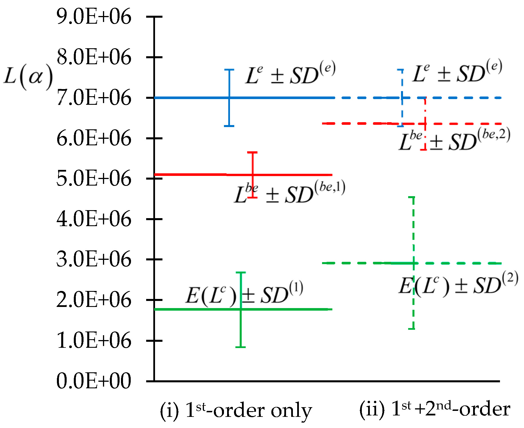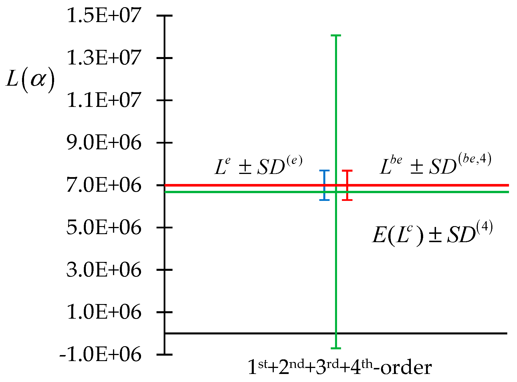The unmatched guaranteed reduction in predicted uncertainties in the predicted responses (and model parameters) and the essential impact of higher-order sensitivities has been recently illustrated by Fang and Cacuci [31] by applying the second-BERRU-PM methodology [28,29] to the polyethylene-reflected plutonium OECD/NEA reactor physics benchmark, which was already described briefly in Section 3.1. The results predicted by using Equations (23) and (28) in conjunction with typical measurement uncertainties (relative standard deviation of 10%) and typical uncertainties (relative standard deviation of 5%) for the total cross-sections (which are the model parameters considered in this illustrative example) are presented in Figure 3 and Figure 4, below. The leakage of neutrons through the outer sphere of the plutonium benchmark is denoted by the letter “L” in Figure 3 and Figure 4. In Figure 3 and Figure 4, the superscript “e” denotes “experimentally measured quantities”, while the superscript “be” denotes “best-estimate optimally predicted quantities”. The standard deviation of the experimentally measured response is denoted as $S{D}^{\left(e\right)}$; the standard deviation of the computed response is denoted as $S{D}^{\left(i\right)}$, and the “best-estimate” standard deviation of the best-estimate response is denoted as $S{D}^{\left(be,i\right)}$. The values 1, 2, and 4, taken on by the index “i” in the superscripts of these standard deviations, correspond, respectively, to the inclusion of only the first-order sensitivities, the inclusion of the first- and the second-order sensitivities, and the inclusion of the first + second + third + fourth-order sensitivities. The parameters (microscopic group-averaged total cross-sections) considered for obtaining the results depicted in Figure 3 and Figure 4 were considered to be uncorrelated and normally distributed, having uniform relative standard deviations of 5%.

The numerical results [in units of $\mathrm{n}\mathrm{e}\mathrm{u}\mathrm{t}\mathrm{r}\mathrm{o}\mathrm{n}\mathrm{s}/\mathrm{s}$] that correspond to the graphs in Figure 3 and Figure 4 are as follows: $E(L^c)\pm S{D}^{\left(1\right)}=1.765\times {10}^6\pm 9.246\times {10}^5$; $L^{be}\pm S{D}^{\left(be,1\right)}=5.093\times {10}^6\pm 5.581\times {10}^5$; $E(L^c)\pm S{D}^{\left(2\right)}=2.914\times {10}^6\pm 1.629\times {10}^6$; $L^{be}\pm S{D}^{\left(be,2\right)}=6.363\times {10}^6\pm 6.431\times {10}^5$; $E(L^c)\pm S{D}^{\left(4\right)}=6.681\times {10}^6\pm 7.386\times {10}^6$; $L^{be}\pm S{D}^{\left(be,4\right)}=6.997\times {10}^6\pm 6.969\times {10}^5$; $L^e\pm S{D}^{(e)}=7.000\times {10}^6\pm 7.000\times {10}^5$.

These results depicted in Figure 3 and Figure 4 imply the following conclusions:

(i) The nominal (value of the) computed response, $L^c$, coincides with the expected value of the computed response, $E(L^c)$, only if all sensitivities higher than first-order are ignored. Otherwise, the effects of the second- and higher-order sensitivities cause the expected value of the computed response, $E(L^c)$, to be increasingly larger than the nominal computed value $L^c$, i.e., $E(L^c)\ge L^c$;

(ii) As indicated in Figure 3, the inclusion of only the first- and second-order sensitivities appears to indicate that the “computations are inconsistent with the computations” since, in these cases, the standard deviation of the measured response does not overlap with the standard deviation of the computed response. However, this indication is proven to be false by the result depicted in Figure 4, which shows that the inclusion of the third- and fourth-order sensitivities renders the computation to be “consistent” with the measurement. This situation underscores the importance of including not only the second-order but also the higher (third- and fourth) order sensitivities;

(iii) As predicted by the second-BERRU-PM methodology, the best-estimate response value, $L^{be}$, always falls in between the “expected value of the computed response”, $E(L^c)$, and the experimentally measured value $L^e$, i.e., $E(L^c)<L^{be}<L^e$. As higher-order sensitivities are included, the predicted response value, $L^{be}$, approaches the experimentally measured value, $L^{be}$. Remarkably, all three of these quantities become clustered together, with $L^{be}\cong L^e$, when all sensitivities, from first to fourth order, are included;

(iv) It is also apparent that the predicted standard deviation of the predicted response is smaller than either the originally computed response standard deviation or the measured response standard deviation, i.e., $S{D}^{\left(be,1\right)}<S{D}^{(e)}$ and $S{D}^{\left(be,1\right)}<S{D}^{\left(1\right)}$. This reduction in the magnitude of the predicted response standard deviation is guaranteed by the application of the second-BERRU-PM methodology; this reduction is even more accentuated when the higher (second-, third-, fourth-) order sensitivities are also included;

(v) The results depicted in Figure 3 and Figure 4 also indicate that the second-order response sensitivities must always be included, even if only to quantify the need for including (or not) the third- and/or fourth-order sensitivities;

(vi) As indicated in Figure 3 and Figure 4, the standard deviation of the computed response increases as sensitivities of increasingly higher order are incorporated, as would logically be expected. However, this fact has no negative consequences after the second-BERRU-PM methodology is applied to combine the computational results with the experimental results since, as shown in Figure 3 and Figure 4, the second-BERRU-PM methodology reduces the predicted best-estimate standard deviations to values that are smaller than both the computed and the experimentally measured values of the initial standard deviations. The results obtained confirm the fact that the second-BERRU-PM methodology predicts best-estimate results that fall in between the corresponding computed and measured values while reducing the predicted standard deviations of the predicted results to values smaller than either the experimentally measured or the computed values of the respective standard deviations.

The second-BERRU-PM methodology also yields best-estimate optimal values for the (posterior) calibrated parameters, as indicated in Equation (26), along with reduced predicted uncertainties (standard deviations) for the predicted parameters, as shown in Equation (29). The best-estimate calibrated parameters thus obtained are subsequently used in the respective calibrated computational models to compute best-estimate responses, which will have smaller uncertainties since the calibrated parameters have smaller uncertainties than the original uncalibrated parameters. Such subsequent computations yield results practically equivalent to the predicted response value $L^{be}$ and the predicted best-estimate reduced standard deviation $S{D}^{\left(be,4\right)}$; because of the page limitation, however, these results cannot be reproduced here.

Fundamental Advantages of the Second-BERRU-PM Methodology over the Second-Order Data Assimilation

This section will describe the decisive advantages of the second-BERRU-PM methodology over the Second-Order Data Assimilation methodology. The Second-Order Data Assimilation methodology relies on using the second-order procedure to minimize a user-defined functional, which is meant to represent, in a chosen norm (usually the energy norm), the discrepancies between computed and experimental results (“responses”). The “Second-Order Data Assimilation” [32,33] considers that the vector of measured responses (“observations”), denoted by the vector $z\triangleq {\left(z_1,\dots ,z_{TR}\right)}^{†}$, is a known function of the vector of state-variables $u\left(x\right)\triangleq {\left[u_1\left(x\right),\dots ,u_{TD}\left(x\right)\right]}^{†}$ and the vector of errors $w\triangleq {\left(w_1,\dots ,w_{TR}\right)}^{†}$, having the expression: $z=h\left(u\right)+w$, where $u$ denotes the vector of dependent variables, and $h\left(u\right)\triangleq {\left[h_1\left(u\right),\dots ,h_{TR}\left(u\right)\right]}^{†}$ is a known vector-function of $u$. The error term, $w$, is considered here to include “representative errors” stemming from sampling and grid interpolation; the mean value of $w$ corresponds to $r_e\triangleq {\left(r_1^e,\dots ,r_{TR}^e\right)}^{†}$, and the covariance matrix of $w$ corresponds to $C_e^{rr}$. As described in [32,33], $w$ is often considered to have the characteristics of “white noise”, in which case, $z\sim N\left[h\left(u\right),C_e^{rr}\right]$ is a normal distribution with mean $h\left(u\right)$ and covariance $C_e^{rr}$. In addition, it is assumed that the prior “background” information is also known, being represented by a multivariate normal distribution with a known mean, denoted as $u_b$, and a known covariance matrix denoted as $B$, i.e., $u\sim N\left[u_b,B\right]$. The posterior distribution, $p\left(z|u\right)$, is obtained by applying Bayes’ Theorem to the above information, which yields the result $p\left(z|u\right)\sim \exp \left[-J\left(u\right)\right]$, where $J\left(u\right)\triangleq \frac{1}{2}\left\{{\left[z-h\left(u\right)\right]}^{†}{\left(C_e^{rr}\right)}^{-1}\left[z-h\left(u\right)\right]+{\left(u-u_b\right)}^{†}{B}^{-1}\left(u-u_b\right)\right\}$. The maximum posterior estimate is obtained by determining the minimum of the functional $J\left(u\right)$, which occurs at the root(s) of the following equation:

$$0=\nabla J\left(u\right)=B^{-1}\left(u-u_b\right)-{\left[D_h\left(u\right)\right]}^{†}{\left(C_e^{rr}\right)}^{-1}\left[z-h\left(u\right)\right],$$

(32)

where $D_h\left(u\right)$ denotes the Jacobian matrix of $h\left(u\right)$ with respect to the components of $u$.

The “first-order data assimilation” procedure solves Equation (32) by using a “partial quadratic approximation” to $J\left(u\right)$, while the “second-order data assimilation” procedure solves Equation (32) by using a “full quadratic approximation” to $J\left(u\right)$, as detailed in [32,33], to obtain the “optimal data assimilation solution”, which is here denoted as $u_{DA}$, as the solution of Equation (32). The following fundamental differences become apparent by comparing the “Data Assimilation” result represented by Equation (32) and the Hi-BERRU-PM results.

1. Data assimilation (DA) is formulated conceptually [32,33] either only in the phase space of measured responses (“observation space formulation”) or only in the phase space of the model’s dependent variables (“state space formulation”). Hence, DA can calibrate initial conditions as “direct results” but cannot directly calibrate any other model parameters. In contradistinction, the second-BERRU-PM methodology is formulated conceptually in the most inclusive “joint phase space of parameters, computed and measured responses”. Consequently, the second-BERRU-PM methodology simultaneously calibrates responses and parameters, thus simultaneously providing results for forward and inverse problems;

2. If the experiments are perfectly well known, i.e., if $C_e^{rr}=0$, Equation (32) indicates that the DA methodology fails fundamentally. In contradistinction, Equations (23)–(31) indicate that the second-BERRU-PM methodology does not fail when $C_e^{rr}=0$ because, in any situation, $C_c^{rr}\ne 0$;

3. The DA methodology also fails fundamentally when the response measurements happen to coincide with the computed value of the response, i.e., when $z=h\left(u\right)$ is at some point in the state space. In such a case, the DA’s Equation (32) yields the trivial result $u_{DA}=u_b$. In contradistinction, the Hi-BERRU-PM methodology does not yield such a trivial result when the response measurements happen to coincide with the computed value of the response, i.e., when $r_e=r_k\left({\alpha }^0\right)$, because the difference $E_c\left(r\right)-r_e$, which appears on the right sides of Equations (23), (26) and (28)–(31), remains non-zero due to the contributions of the second- and higher-order sensitivities of the responses with respect to the model parameters, since ${\left\{E_c\left(r_k\right)-r_k^e\right\}}_{r_k^e=r_k\left({\alpha }^0\right)}={\displaystyle \sum _{i=1}^{TP}{\displaystyle \sum _{j=1}^{TP}{\left\{{\partial }^2{r}_k\left(\alpha \right)/\partial {\alpha }_i\partial {\alpha }_j\right\}}_{{\alpha }^0}\mathrm{cov}\left({\alpha }_i,{\alpha }_j\right)/2}}+\dots \dots \ne 0$ for $k=1,\dots ,TR$. This situation clearly underscores the need for computing and retaining (at least) the second-order response sensitivities to the model parameters. Although a situation when $r_e=r_k\left({\alpha }^0\right)$ is not expected to occur frequently in practice, there are no negative consequences (should such a situation occur) if the second-BERRU-PM methodology is used, in contradistinction to using the DA methodology;

4. The second-BERRU-PM methodology only requires the inversion of the matrix $\left(C_e^{rr}+C_c^{rr}\right)$ of size $TR\times TR$. In contradistinction, the solution of the “first-order DA” requires the inversion of the Jacobian $D_h\left(u\right)$ of $h\left(u\right)$, while the solution of the “second-order DA” also requires the inversion of a matrix-vector product involving the Hessian matrix of $h\left(u\right)$; these matrices are significantly larger [32,33] than the matrix $\left(C_e^{rr}+C_c^{rr}\right)$. Hence, the second-BERRU-PM methodology is significantly more efficient computationally than DA;

5. The DA methodology [32,33] is practically non-extendable beyond “second-order”. A “third-order DA” would be computationally impractical because of the massive sizes of the matrices that would need to be inverted. In contradistinction, the second-BERRU-PM methodology presented herein already comprises the fourth-order sensitivities of responses to parameters and can be readily extended/generalized to include even higher-order sensitivities and parameter correlations.

All of the above advantages of the second-BERRU-PM methodology over the DA methodology stem from the fact that the second-BERRU-PM methodology is fundamentally anchored in physics-based principles (thermodynamics and information theory) formulated in the most inclusive possible phase space (namely, the combined phase space of computed and measured parameters and responses), whereas the DA methodology [32,33] is fundamentally based on the minimization of a subjective user-chosen functional.

4. Critical Review of Methods for Computing High-Order Sensitivities

There are only two methodologies for computing directly high-order functional derivatives, i.e., sensitivities, of a model response to the model’s underlying parameters, namely, (i) the well-known finite difference (FD) approximations of derivatives in conjunction with re-computations with altered parameter values and (ii) the “nth-Order Comprehensive Adjoint Sensitivity Analysis Methodology” (nth CASAM) developed by Cacuci [21,23]. The salient features of the nth CASAM methodology will be reviewed in Section 4.1, while the most important issues encountered when using FD approximations will be highlighted in Section 4.2 below. A number of quasi-statistical methods also exist for computing so-called “sensitivity indicators”, which are not functional derivatives of the response with respect to the model parameters but are attempts at extracting sensitivity-like information from the approximate response-covariance-like information obtained from many re-computations (occasionally using Monte Carlo methods). Conceptually, these statistical methods are the equivalent of attempting to disentangle “sensitivities” within the components of the right side of Equation (25) from a statistical approximation of the left side of Equation (25). The salient features of these statistical methods will be briefly discussed in Section 4.3 below.

4.1. The Only Method for Efficiently Computing Exact Expressions of High-Order Sensitivities: The nth-CASAM

The only extant method that overcomes, to the largest possible extent, the curse of dimensionality while providing exact expressions for computing efficiently sensitivities of all orders is the “nth-Order Comprehensive Adjoint Sensitivity Analysis Methodology (nth-CASAM)” developed by Cacuci [21,23] by extending the original adjoint sensitivity analysis methodology conceived by Cacuci [1,2]. The nth-CASAM requires computations in linearly increasing higher-dimensional Hilbert spaces, as opposed to exponentially increasing parameter-dimensional spaces. In particular, for a scalar-valued response associated with a model comprising $TP$ model parameters, the nth-CASAM requires one adjoint computation for computing exactly all of the first-order response sensitivities, as opposed to at least $TP$ forward computations, as required by other methods to obtain approximate values for these sensitivities.

The starting point of the mathematical framework of the nth-CASAM commences by noting that the known nominal (or mean) parameter values, ${\alpha }^0$, will differ from the true values $\alpha$, which are unknown, by variations $\delta \alpha \triangleq {\left(\delta {\alpha }_1,\dots ,\delta {\alpha }_{TP}\right)}^{†}$, where $\delta {\alpha }_i\triangleq {\alpha }_i-{\alpha }_i^0$. The parameter variations $\delta \alpha$ will induce variations $v^{\left(1\right)}\left(x\right)\triangleq {\left[\delta u_1\left(x\right),\dots ,\delta u_{TD}\left(x\right)\right]}^{†}$ around the nominal solution $u^0\left(x\right)$ in the forward state functions via Equations (1) and (2). In turn, these variations will induce variations in the system’s response $R\left[u\left(x\right);\alpha \right]$. Mathematically, the response variations are represented by the first-order G-differential $\delta R\left[u^0\left(x\right);{\alpha }^0;v^{\left(1\right)}\left(x\right);\delta \alpha \right]$ of the response $R\left[u\left(x\right);\alpha \right]$ induced by arbitrary variations $\left[v^{\left(1\right)}\left(x\right);\delta \alpha \right]$ in a neighborhood around the nominal functions and parameter values $\left[u^0\left(x\right);{\alpha }^0\right]$, and is defined as follows:

$$\delta R\left[u^0\left(x\right);{\alpha }^0;v^{\left(1\right)}\left(x\right);\delta \alpha \right]\triangleq {\left\{\frac{d}{d\epsilon }R\left[u^0+\epsilon v^{\left(1\right)};{\alpha }^0+\epsilon \left(\delta \alpha \right)\right]\right\}}_{\epsilon =0},$$

(33)

where $\epsilon$ is a scalar quantity. The G-variation $\delta R\left[u^0\left(x\right);{\alpha }^0;v^{\left(1\right)}\left(x\right);\delta \alpha \right]$ is an operator defined on the same domain as $R\left[u\left(x\right);\alpha \right]$ and has the same range as $R\left[u\left(x\right);\alpha \right]$. The existence of the G-variation $\delta R\left[u^0\left(x\right);{\alpha }^0;v^{\left(1\right)}\left(x\right);\delta \alpha \right]$ does not guarantee its numerical computability. Numerical methods most often require that $\delta R\left[u^0\left(x\right);{\alpha }^0;v^{\left(1\right)}\left(x\right);\delta \alpha \right]$ be linear in $\left[v^{\left(1\right)}\left(x\right);\delta \alpha \right]$ in a neighborhood $\left[u^0+\epsilon v^{\left(1\right)};{\alpha }^0+\epsilon \left(\delta \alpha \right)\right]$ around $\left[u^0\left(x\right);f^0\left(\alpha \right)\right]$, thereby admitting a total first-order G-derivative, which will be denoted as $dR\left[u^0\left(x\right);{\alpha }^0;v^{\left(1\right)}\left(x\right);\delta \alpha \right]$. In practice, the computation of the expression on the right side of Equation (33) reveals immediately if the respective expression is linear (or not) in the vectors $v^{\left(1\right)}\left(x\right)$ and/or $\delta \alpha$. Numerical methods (e.g., Newton’s method and variants thereof) for solving Equations (1) and (2) also require the existence of the first-order G-derivatives of the original model equations. Therefore, it will be henceforth assumed that the model responses and the operators underlying the physical system modeled by Equations (1) and (2) admit G-derivatives.

The first-order G-derivative $dR\left[u^0\left(x\right);{\alpha }^0;v^{\left(1\right)}\left(x\right);\delta \alpha \right]$ of $R\left[u\left(x\right);\alpha \right]$ is obtained, by definition, as follows:

$$\begin{array}{l}dR\left[u^0\left(x\right);{\alpha }^0;v^{\left(1\right)}\left(x\right);\delta \alpha \right]\triangleq {\left\{dR\left[u\left(x\right);x;\delta \alpha \right]\right\}}_{dir}+{\left\{dR\left[u\left(x\right);\alpha ;v^{\left(1\right)}\left(x\right)\right]\right\}}_{ind}\\ \triangleq {\left\{\frac{d}{d\epsilon }{\displaystyle \underset{{\lambda }_1\left({\alpha }^0\right)+\epsilon \left(\delta {\lambda }_1\right)}{\overset{{\omega }_1\left({\alpha }^0\right)+\epsilon \left(\delta {\omega }_1\right)}{\int }}\dots {\displaystyle \underset{{\lambda }_{TI}\left({\alpha }^0\right)+\epsilon \left(\delta {\lambda }_{TI}\right)}{\overset{{\omega }_{TI}\left({\alpha }^0\right)+\epsilon \left(\delta {\omega }_{TI}\right)}{\int }}S\left[u^0+\epsilon v^{\left(1\right)},{\alpha }^0+\epsilon \left(\delta \alpha \right);x\right]d{x}_1\dots d{x}_{TI}}}\right\}}_{\epsilon =0}.\end{array}$$

(34)

In Equation (34), the “direct effect” term ${\left\{\delta R\left[u\left(x\right);x;\delta \alpha \right]\right\}}_{dir}$ comprises only dependencies on $\delta \alpha$ and is defined as follows:

$${\left\{\delta R\left[u\left(x\right);x;\delta \alpha \right]\right\}}_{dir}\triangleq {\left\{\frac{\partial R\left(u;f\right)}{\partial \alpha }\right\}}_{{\alpha }^0}\delta \alpha \triangleq {\displaystyle \sum _{j_1=1}^{TF}{\left\{R^{\left(1\right)}\left[j_1;u\left(x\right);\alpha \right]\right\}}_{dir}\delta {\alpha }_{j_1}},$$

(35)

where

$$\begin{array}{l}{\left\{R^{\left(1\right)}\left[j_1;u\left(x\right);\alpha \right]\right\}}_{dir}\triangleq {\left\{{\displaystyle \underset{{\lambda }_1\left(\alpha \right)}{\overset{{\omega }_1\left(\alpha \right)}{\int }}\dots {\displaystyle \underset{{\lambda }_{TI}\left(\alpha \right)}{\overset{{\omega }_{TI}\left(\alpha \right)}{\int }}\frac{\partial S\left(u;\alpha ;\alpha \right)}{\partial {\alpha }_{j_1}}d{x}_1\dots d{x}_{TI}}}\right\}}_{{\alpha }^0}\\ +{\displaystyle \sum _{j=1}^{TI}{\left\{\frac{\partial {\omega }_j\left(\alpha \right)}{\partial {\alpha }_{j_1}}{\displaystyle \underset{{\lambda }_1}{\overset{{\omega }_1}{\int }}d{x}_1\dots {\displaystyle \underset{{\lambda }_{j-1}}{\overset{{\omega }_{j-1}}{\int }}d{x}_{i-1}{\displaystyle \underset{{\lambda }_{j+1}}{\overset{{\omega }_{j+1}}{\int }}d{x}_{i+1}\dots {\displaystyle \underset{{\lambda }_{TI}}{\overset{{\omega }_{TI}}{\int }}d{x}_{TI}S\left[u\left(x_1\hspace{1em},.,{\omega }_j\left(\alpha \right),.,x_{N_x}\right);\alpha \right]}}}}\right\}}_{{\alpha }^0}}\\ -{\displaystyle \sum _{j=1}^{TI}{\left\{\frac{\partial {\lambda }_j\left(\alpha \right)}{\partial {\alpha }_{j_1}}{\displaystyle \underset{{\lambda }_1}{\overset{{\omega }_1}{\int }}d{x}_1\dots {\displaystyle \underset{{\lambda }_{j-1}}{\overset{{\omega }_{j-1}}{\int }}d{x}_{i-1}{\displaystyle \underset{{\lambda }_{j+1}}{\overset{{\omega }_{j+1}}{\int }}d{x}_{i+1}\dots {\displaystyle \underset{{\lambda }_{TI}}{\overset{{\omega }_{TI}}{\int }}d{x}_{TI}S\left[u\left(x_1\hspace{1em},.,{\lambda }_j\left(\alpha \right),.,x_{N_x}\right);\alpha \right]}}}}\right\}}_{{\alpha }^0}}.\end{array}$$

(36)

$${\left\{\delta R\left[u\left(x\right);\alpha ;v^{\left(1\right)}\left(x\right)\right]\right\}}_{ind}\triangleq {\left\{{\displaystyle \underset{{\lambda }_1\left(\alpha \right)}{\overset{{\omega }_1\left(\alpha \right)}{\int }}d{x}_1\dots {\displaystyle \underset{{\lambda }_{TI}\left(\alpha \right)}{\overset{{\omega }_{TI}\left(\alpha \right)}{\int }}d{x}_{TI}\frac{\partial S\left(u;\alpha \right)}{\partial u}{v}^{\left(1\right)}\left(x\right)}}\right\}}_{{\alpha }^0}$$

(37)

The direct effect term can be computed directly by using Equation (36). In contradistinction, the indirect effect term can be quantified only after having determined the variations $v^{\left(1\right)}\left(x\right)$ in terms of the variations $\delta \alpha$. The first-order relationship between the vectors $v^{\left(1\right)}\left(x\right)$ and the parameter variations $\delta \alpha$ is determined by solving the equations obtained by applying the definition of the G-differential to Equations (1) and (2), which yields the following equations:

$${\left\{\frac{d}{d\epsilon }N\left[u^0+\epsilon v^{\left(1\right)}\left(x\right);{\alpha }^0+\epsilon \left(\delta \alpha \right)\right]\right\}}_{\epsilon =0}={\left\{\frac{d}{d\epsilon }Q\left[x;{\alpha }^0+\epsilon \left(\delta \alpha \right)\right]\right\}}_{\epsilon =0},$$

(38)

$${\left\{\frac{d}{d\epsilon }B\left[u^0+\epsilon v^{\left(1\right)}\left(x\right);{\alpha }^0+\epsilon \left(\delta \alpha \right)\right]\right\}}_{\epsilon =0}-{\left\{\frac{d}{d\epsilon }C\left[{\alpha }^0+\epsilon \left(\delta \alpha \right)\right]\right\}}_{\epsilon =0}=0.$$

(39)

Carrying out the differentiations with respect to $\epsilon$ in Equations (38) and (39) and setting $\epsilon =0$ in the resulting expressions yields the following equations:

$${\left\{N^{\left(1\right)}\left(u;\alpha \right)v^{\left(1\right)}\left(j_1;x\right)\right\}}_{{\alpha }^0}={\left\{s_V^{\left(1\right)}\left(j_1;u;\alpha \right)\right\}}_{{\alpha }^0},\hspace{1em}{j}_1=1,\dots ,TP;\hspace{1em}x\in {\mathsf{\Omega }}_x,$$

(40)

$${\left\{b_V^{\left(1\right)}\left[u;\alpha ;v^{\left(1\right)}\left(j_1;x\right)\right]\right\}}_{{\alpha }^0}=0;\hspace{1em}{j}_1=1,\dots ,TP;\hspace{1em}x\in \partial {\mathsf{\Omega }}_x\left({\alpha }^0\right).$$

(41)

In Equations (40) and (41), the superscript “(1)” indicates the “first-level” and the various quantities which appear in these equations are defined as follows:

$$N^{\left(1\right)}\left(u;\alpha \right)\triangleq \left\{\frac{\partial N\left(u;\alpha \right)}{\partial u}\right\}\triangleq {\left\{\frac{\partial N_i}{\partial u_j}\right\}}_{TD\times TD};$$

(42)

$$s_V^{\left(1\right)}\left(j_1;u;\alpha \right)\triangleq \frac{\partial \left[Q\left(\alpha \right)-N\left(u;\alpha \right)\right]}{\partial {\alpha }_{j_1}};$$

(43)

$${\left\{b_V^{\left(1\right)}\left[u;\alpha ;v^{\left(1\right)}\left(j_1;x\right)\right]\right\}}_{{\alpha }^0}\triangleq {\left\{\frac{\partial B\left(u;\alpha \right)}{\partial u}{v}^{\left(1\right)}\left(j_1;x\right)+\frac{\partial \left[B\left(u;\alpha \right)-C\left(\alpha \right)\right]}{\partial {\alpha }_{j_1}}\right\}}_{{\alpha }^0}.$$

(44)

The system of equations comprising Equations (40) and (41) is called the “First-Level Variational Sensitivity System” (first-LVSS). As Equations (40) and (41) indicate, every parameter variation $\delta {\alpha }_{j_1}$, $j_1=1,\dots ,TP$, will induce, directly or indirectly, variations in the model’s state variables. In principle, therefore, for every parameter variation $\delta {\alpha }_{j_1}$, $j_1=1,\dots ,TP$, there would correspond a solution $v^{\left(1\right)}\left(j_1;x\right)$, $j_1=1,\dots ,TP$, of the first-LVSS. Thus, if the effect of every parameter variation were of interest, then the first-LVSS would need to be solved $TP$ times, with distinct right-side and boundary conditions for each parameter variation $\delta {\alpha }_{j_1}$, which would require at least $TP$ large-scale computations.

However, solving the first-LVSS can be avoided altogether by using the ideas underlying the “adjoint sensitivity analysis methodology” conceived by Cacuci [1,2] for the most efficient computation of exact expressions of first-order sensitivities, and subsequently, generalized by Cacuci [21,23] to enable the computation of arbitrarily high-order response sensitivities to model parameters. Thus, the need for computing the vectors $v^{\left(1\right)}\left(j_1;x\right)$ and $j_1=1,\dots ,TP$ is eliminated by expressing the indirect effect term defined in Equation (37) in terms of the solutions of the “First-Level Adjoint Sensitivity System” (First-LASS), the construction of which requires the introduction of adjoint operators. Constructing the First-LASS is accomplished by introducing a (real) Hilbert space denoted as ${\mathrm{H}}_1\left({\mathsf{\Omega }}_x\right)$, endowed with an inner product of two vectors $w^{(1)}\left(x\right)\in {\mathrm{H}}_1$ and $w^{(2)}\left(x\right)\in {\mathrm{H}}_1$, which is denoted as ${\langle w^{(1)},w^{(2)}\rangle }_1$ and defined as follows:

$${\langle w^{(1)},w^{(2)}\rangle }_1\triangleq {\left\{{\displaystyle \underset{{\lambda }_1\left(\alpha \right)}{\overset{{\omega }_1\left(\alpha \right)}{\int }}\dots {\displaystyle \underset{{\lambda }_{TI}\left(\alpha \right)}{\overset{{\omega }_{TI}\left(\alpha \right)}{\int }}\left[w^{(1)}\left(x\right)·w^{(2)}\left(x\right)\right]d{x}_1\dots d{x}_{TI}}}\right\}}_{{\alpha }^0},$$

(45)

where $w^{(1)}\left(x\right)·w^{(1)}\left(x\right)\triangleq {\displaystyle \sum _{i=1}^{TD}{w}_i^{(1)}\left(x\right)w_i^{(2)}}\left(x\right)$, and where the “dagger” ($†$), which indicates “transposition”, has been omitted (to simplify the notation) in the representation of this scalar product.

Consider a vector $a^{(1)}\left(x\right)\in {\mathrm{H}}_1$, which is an element in ${\mathrm{H}}_1\left({\mathsf{\Omega }}_x\right)$ but is otherwise arbitrary at this stage, and use Equation (45) to form the inner product of $a^{(1)}\left(x\right)\in {\mathrm{H}}_1$ with the relation provided in Equation (40) to obtain

$${\left\{{\langle a^{(1)},N^{\left(1\right)}\left(u;\alpha \right)v^{\left(1\right)}\rangle }_1\right\}}_{{\alpha }^0}={\left\{{\langle a^{(1)},q_V^{\left(1\right)}\left(u;\alpha ;\delta \alpha \right)\rangle }_1\right\}}_{{\alpha }^0},x\in {\mathsf{\Omega }}_x.$$

(46)

The left side of Equation (46) is transformed by using the definition of the adjoint operator in ${\mathrm{H}}_1\left({\mathsf{\Omega }}_x\right)$ as follows:

$${\left\{{\langle a^{(1)},N^{\left(1\right)}\left(u;\alpha \right)v^{\left(1\right)}\rangle }_1\right\}}_{{\alpha }^0}={\left\{{\langle A^{\left(1\right)}\left(u;\alpha \right)a^{(1)},v^{\left(1\right)}\rangle }_1\right\}}_{{\alpha }^0}+{\left\{{\left[P^{\left(1\right)}\left(u;\alpha ;v^{\left(1\right)};a^{(1)}\right)\right]}_{\partial {\mathsf{\Omega }}_x}\right\}}_{{\alpha }^0},$$

(47)

where ${\left[P^{\left(1\right)}\left(u;\alpha ;a^{(1)};v^{\left(1\right)}\right)\right]}_{\partial {\mathsf{\Omega }}_x}$ denotes the associated bilinear concomitant evaluated on the domain’s boundary $\partial {\mathsf{\Omega }}_x$, and $A^{\left(1\right)}\left(u;\alpha \right)\triangleq {\left[N^{\left(1\right)}\left(u;\alpha \right)\right]}^{*}$ denotes the operator formally adjoint to $N^{\left(1\right)}\left(u;g\right)$. The symbol ${\left[\right]}^{\ast }$ indicates “formal adjoint” operator.

The first term on the right side of Equation (47) is required to represent the indirect effect term defined in Equation (37) by imposing the following relationship:

$${\left\{A^{\left(1\right)}\left(u;\alpha \right)a^{\left(1\right)}\left(x\right)\right\}}_{{\alpha }^0}={\left\{\partial S\left(u;\alpha \right)/\partial u\right\}}_{{\alpha }^0}\triangleq q_A^{\left(1\right)}\left[u\left(x\right);\alpha \right],x\in {\mathsf{\Omega }}_x.$$

(48)

The domain of $A^{\left(1\right)}\left(u;\alpha \right)$ is determined by selecting appropriate adjoint boundary and/or initial conditions, which will be denoted in operator form as:

$${\left\{b_A^{\left(1\right)}\left(u;a^{\left(1\right)};\alpha \right)\right\}}_{{\alpha }^0}=0,x\in \partial {\mathsf{\Omega }}_x.$$

(49)

The above boundary conditions for the adjoint operator $A^{\left(1\right)}\left(u;\alpha \right)$ are obtained by imposing the following requirements: (i) they must be independent of unknown values of V⁽¹⁾(x) and $\delta \alpha$; (ii) the substitution of the boundary and initial conditions represented by Equations (41) and (49) into the expression of ${\left\{{\left[P^{\left(1\right)}\left(u;\alpha ;v^{\left(1\right)};a^{(1)}\right)\right]}_{\partial {\mathsf{\Omega }}_x}\right\}}_{{\alpha }^0}$ must cause all terms containing unknown values of $v^{\left(1\right)}\left(x\right)$ to vanish.

Using the adjoint and forward variational boundary conditions represented by Equations (49) and (41) into Equation (47) reduces the bilinear concomitant ${\left\{{\left[P^{\left(1\right)}\left(u;\alpha ;v^{\left(1\right)};a^{(1)}\right)\right]}_{\partial {\mathsf{\Omega }}_x}\right\}}_{{\alpha }^0}$ to a residual bilinear concomitant denoted as ${\left\{{\left[{\widehat{P}}^{\left(1\right)}\left(u;\alpha ;a^{(1)};\delta \alpha \right)\right]}_{\partial {\mathsf{\Omega }}_x}\right\}}_{{\alpha }^0}$, which will contain boundary terms involving only known values of $\delta \alpha$, $u$, and $a^{(1)}$. The residual bilinear concomitant ${\left\{{\left[{\widehat{P}}^{\left(1\right)}\left(u;\alpha ;a^{(1)};\delta \alpha \right)\right]}_{\partial {\mathsf{\Omega }}_x}\right\}}_{{\alpha }^0}$ is linear in $\delta \alpha$. The results obtained in Equations (47) and (48) are now used together with Equation (37) to obtain the following expression of the indirect-effect term as a function of $a^{(1)}\left(x\right)$:

$$\begin{array}{l}{\left\{\delta R\left[u\left(x\right);\alpha ;v^{\left(1\right)}\left(x\right);\delta \alpha \right]\right\}}_{{\alpha }^0}={\left\{\delta R\left[u\left(x\right);\alpha ;\delta \alpha \right]\right\}}_{dir}+{\left\{{\langle a^{(1)},q_V^{\left(1\right)}\left(u;\alpha ;\delta \alpha \right)\rangle }_1\right\}}_{{\alpha }^0}\\ -{\left\{{\left[{\widehat{P}}^{\left(1\right)}\left(u;\alpha ;a^{(1)};\delta \alpha \right)\right]}_{\partial {\mathsf{\Omega }}_x}\right\}}_{{\alpha }^0}\triangleq {\displaystyle \sum _{j_1=1}^{TP}{\left\{R^{\left(1\right)}\left[j_1;u\left(x\right);a^{(1)}\left(x\right);\alpha \right]\right\}}_{{\alpha }^0}\delta {\alpha }_{j_1}},\end{array}$$

(50)

where, for each $j_1=1,\dots ,TP$, the quantity $R^{\left(1\right)}\left[j_1;u\left(x\right);a^{\left(1\right)}\left(x\right);\alpha \right]\triangleq \partial R\left[\mathbf{u}\right(\mathbf{x});\alpha ]/\partial {\alpha }_{j1}$ denotes the first-order sensitivities of the response $R\left[u\left(x\right);\alpha \right]$ with respect to the model parameters ${\alpha }_{j_1}$ and has the following expression, for $j_1=1,\dots ,TP$:

$$\begin{array}{l}{R}^{\left(1\right)}\left[j_1;u\left(x\right);a^{\left(1\right)}\left(x\right);\alpha \right]={\left\{R^{\left(1\right)}\left[j_1;u\left(x\right);\alpha \right]\right\}}_{dir}-\frac{\partial {\left[{\widehat{P}}^{\left(1\right)}\left(u;a^{(1)};\alpha ;\right)\right]}_{\partial {\mathsf{\Omega }}_x}}{\partial {\alpha }_{j_1}}\\ +{\displaystyle \underset{{\lambda }_1\left(\alpha \right)}{\overset{{\omega }_1\left(\alpha \right)}{\int }}d{x}_1\dots {\displaystyle \underset{{\lambda }_{TI}\left(\alpha \right)}{\overset{{\omega }_{TI}\left(\alpha \right)}{\int }}{a}^{(1)}\left(x\right)\frac{\partial \left[Q\left(\alpha \right)-N\left(u;\alpha \right)\right]}{\partial {\alpha }_{j_1}}d{x}_{TI}}}\triangleq \frac{\partial R\left[u\left(x\right);\alpha \right]}{\partial {\alpha }_{j_1}}.\end{array}$$

(51)

Each of the first-order sensitivities $R^{\left(1\right)}\left[j_1;u\left(x\right);a^{\left(1\right)}\left(x\right);\alpha \right]$ of the response $R\left[u\left(x\right);f\left(\alpha \right)\right]$, with respect to the model parameters to be computed inexpensively after having obtained the first-level adjoint function $a^{(1)}\left(x\right)\in {\mathrm{H}}_1$, using only quadrature formulas to evaluate the various inner products involving $a^{(1)}\left(x\right)\in {\mathrm{H}}_1$ in Equation (51). The function $a^{(1)}\left(x\right)\in {\mathrm{H}}_1$ is obtained by solving numerically (48) and (49), which is the only large-scale computation needed for obtaining all of the first-order sensitivities. Equations (48) and (49) are called the First-Level Adjoint Sensitivity System (first-LASS). The solution, $a^{(1)}\left(x\right)\in {\mathrm{H}}_1\left({\mathsf{\Omega }}_x\right)$, of the First-LASS is called the first-level adjoint function. It is very important to note that the First-LASS is independent of all parameter variations $\delta {\alpha }_{j_1}$,$j_1=1,\dots ,TP$, and, therefore, needs to be solved only once, regardless of the number of model parameters under consideration. Furthermore, since the First-LASS is linear in $a^{(1)}\left(x\right)$, solving it requires less computational effort than solving the original model, which is nonlinear in $u\left(x\right)$.

The second-order sensitivities of the response $R\left[u\left(x\right);f\left(\alpha \right)\right]$, with respect to the model parameters are computed by applying the principles underlying the first-CASAM to each of the first-order sensitivities $R^{\left(1\right)}\left[j_1;u\left(x\right);a^{\left(1\right)}\left(x\right);\alpha \right]$ considered as a “model response”. This way, the second-order sensitivities of $R\left[u\left(x\right);f\left(\alpha \right)\right]$, with respect to the model parameters, are computed in an order of priority chosen by the user (e.g., the largest of the first-order sensitivities would be considered with the highest priority). If all first-order sensitivities are treated as responses, then the mixed second-order sensitivities would be computed twice, using distinct second-level adjoint functions. Thus, the symmetry underlying the mixed higher-order sensitivities provides an intrinsic mutual “verification” of the respective numerical accuracies. The third-order sensitivities are computed by applying the principles of the first-CASAM to the second-order sensitivities, and so on. The details underlying the computations of the second- and higher-order sensitivities will be presented in detail in the accompanying Part II [24] when presenting the newly developed “high-order adjoint sensitivity analysis of responses to functions/features of model parameters” (nth-FASAM), which greatly increases the efficiency of this methodology in special cases.

4.2. Using Finite Differences: A Conceptually Simple but Computationally Inefficient and Inaccurate Procedure for Computing High-Order Sensitivities

Historically, the oldest method for computing approximate values of derivatives of a function of parameters with respect to an underlying parameter, when the actual functional form is not explicitly available, is the use of finite difference formulas in conjunction with re-computations of the respective function (model response) using altered parameter values. Thus, the first-order partial derivative (sensitivity) of a response $R\left(\alpha \right)$, $\alpha \triangleq {\left({\alpha }_1,\dots ,{\alpha }_{TP}\right)}^{†}$ with respect to a parameter ${\alpha }_j$ around the nominal parameter values ${\alpha }^0\triangleq {\left({\alpha }_1^0,\dots ,{\alpha }_i^0,\dots ,{\alpha }_{TP}^0\right)}^{†}$ can be approximately computed by using backward, forward, or central differences; a formula that is accurate to second-order in parameter variations is the following:

$${\left\{\frac{\partial R\left(\alpha \right)}{\partial {\alpha }_j}\right\}}_{{\alpha }^0}\approx \frac{1}{2h_j}\left(R_{j+1}-R_{j-1}\right)+\mathrm{O}\left(h_j^2\right),j=1,\dots ,TP,$$

(52)

where $R_{j+1}\triangleq R\left({\alpha }_j^0+h_j\right)$, $R_{j-1}\triangleq R\left({\alpha }_j^0-h_j\right)$, and where $h_j$ denotes a “judiciously chosen” variation in the parameter ${\alpha }_j$ around its nominal value ${\alpha }_j^0$. The values $R_{j+1}\triangleq R\left({\alpha }_j^0+h_j\right)$ and $R_{j-1}\triangleq R\left({\alpha }_j^0-h_j\right)$ are obtained by re-computing the response $R\left(\alpha \right)$ repeatedly, using the changed parameter values $\left({\alpha }_j^0\pm h_j\right)$. The value of the variation $h_j$ must be chosen by “trial and error” for each parameter ${\alpha }_j$. If $h_j$ is too large or too small, the result produced by Equation (52) will be far off from the exact value of the derivative $\partial R\left(\alpha \right)/\partial {\alpha }_j$. It is important to note that finite difference formulas introduce their intrinsic “methodological errors”, such as the error $\mathrm{O}\left(h_j{}^2\right)$ indicated in Equation (52), which is in addition to and independent of the errors that might be incurred in the computation of $R\left(\alpha \right)$. In other words, even if the computation of $R\left(\alpha \right)$ were perfect (error-free), the finite difference formulas would, nevertheless, introduce their own intrinsic, numerical errors into the computation of the sensitivity $\partial R\left(\alpha \right)/\partial {\alpha }_j$.

For models with many parameters, the computations of approximate sensitivities are expensive, even for the first-order sensitivities; for example, for the PERP benchmark model discussed in Section 3.1, a forward (re)computation requires about 2 min CPU time. The evaluation of the two-point finite difference expression provided in Equation (52) requires two forward transport computations, one forward computation using the altered parameter value $\left({\alpha }_j^0+h_j\right)$ and a second forward computation using the altered parameter value $\left({\alpha }_j^0-h_j\right)$. Hence, the total CPU time needed for computing the 7477 non-zero sensitivities using forward computations in conjunction with the two-point finite difference formula provided in Equation (52) is about 1388 h. In contradistinction, the computation of the first-level adjoint sensitivity function, which is needed to compute all of the first-order sensitivities, takes the same amount of CPU as a forward computation, i.e., ca. 2 min. It is evident that finite difference computations cannot only be performed for specifically targeted sensitivities.

The size of the parameter variation is critically important for the computational accuracy (or lack thereof) of finite difference (FD) formulas, and this importance increases with increasing order of sensitivities. The influence of the size of the parameter variation will be illustrated below by considering the largest fourth-order mixed and, respectively, unmixed sensitivities, namely, (i) the largest fourth-order unmixed relative sensitivity $S^{(4)}\left({\sigma }_{t,6}^{g=30},{\sigma }_{t,6}^{g=30},{\sigma }_{t,6}^{g=30},{\sigma }_{t,6}^{g=30}\right)=2.720\times {10}^6$ for isotope #6 (¹H) of the PERP benchmark and (ii) the largest fourth-order mixed relative sensitivity $S^{(4)}\left({\sigma }_{t,6}^{30},{\sigma }_{t,6}^{30},{\sigma }_{t,6}^{30},{\sigma }_{t,5}^{30}\right)=2.279\times {10}^5$, for the leakage response with respect to the microscopic total cross-sections for group 30 of isotopes #5 (¹²C) and #6 (¹H). The exact values for these sensitivities were computed [22] using the software package the “fourth-order SENS” [34], which computes the first-order through the fourth-order sensitivities of the PERP leakage response with respect to model parameters using the “Fourth-Order Comprehensive Adjoint Sensitivity Analysis Methodology” (fourth-CASAM). On the other hand, the finite difference formula that has been used for computing these sensitivities is reproduced below:

$$\begin{array}{l}\frac{{\partial }^{4}R\left(\alpha \right)}{\partial {\alpha }_{j_1}\partial {\alpha }_{j_2}\partial {\alpha }_{j_3}\partial {\alpha }_{j_4}}\approx \frac{1}{16h_{j_1}{h}_{j_2}{h}_{j_3}{h}_{j_4}}(R_{j_1+1,j_2+1,j_3+1,j_4+1}-R_{j_1+1,j_2+1,j_3+1,j_4-1}-R_{j_1+1,j_2+1,j_3-1,j_4+1}\\ +R_{j_1+1,j_2+1,j_3-1,j_4-1}-R_{j_1+1,j_2-1,j_3+1,j_4+1}+R_{j_1+1,j_2-1,j_3+1,j_4-1}+R_{j_1+1,j_2-1,j_3-1,j_4+1}-R_{j_1+1,j_2-1,j_3-1,j_4-1}\\ -R_{j_1-1,j_2+1,j_3+1,j_4+1}+R_{j_1-1,j_2+1,j_3+1,j_4-1}+R_{j_1-1,j_2+1,j_3-1,j_4+1}-R_{j_1-1,j_2+1,j_3-1,j_4-1}+R_{j_1-1,j_2-1,j_3+1,j_4+1}\\ -R_{j_1-1,j_2-1,j_3+1,j_4-1}-R_{j_1-1,j_2-1,j_3-1,j_4+1}+R_{j_1-1,j_2-1,j_3-1,j_4-1})+O\left(h_{j_1}^2,h_{j_2}^2,h_{j_3}^2,h_{j_4}^2\right),\end{array}$$

(53)

where $R_{j_1+1,j_2+1,j_3+1,j_4+1}\triangleq R\left({\alpha }_{j_1}+h_{j_1},{\alpha }_{j_2}+h_{j_2},{\alpha }_{j_3}+h_{j_3},{\alpha }_{j_4}+h_{j_4}\right)$, etc. The finite difference formulas introduce their intrinsic “methodological errors” of order $\mathrm{O}\left(h_{j_1}^2,h_{j_2}^2,h_{j_3}^2,h_{j_4}^2\right)$, which are in addition to and independent of the errors that might be incurred in the computation of ${\partial }^{4}R\left(\alpha \right)/\partial {\alpha }_{j_1}\partial {\alpha }_{j_2}\partial {\alpha }_{j_3}\partial {\alpha }_{j_4}$.

Finite difference computations of $S^{(4)}\left({\sigma }_{t,6}^{g=30},{\sigma }_{t,6}^{g=30},{\sigma }_{t,6}^{g=30},{\sigma }_{t,6}^{g=30}\right)$ using Equation (53) were performed with step-sizes $h_j$ ranging from 0.125% to 2% of ${\sigma }_{t,6}^{g=30}$. The results of these computations are summarized in

Table 3. Computations of $S^{(4)}\left({\sigma }_{t,6}^{g=30},{\sigma }_{t,6}^{g=30},{\sigma }_{t,6}^{g=30},{\sigma }_{t,6}^{g=30}\right)$ using various step-sizes.

Step-Size ${\mathit{h}}_{\mathit{j}}$	FD-Method	$\frac{\mathit{F}\mathit{D}-4\mathbf{th}\mathit{C}\mathit{A}\mathit{S}\mathit{A}\mathit{M}}{4\mathbf{th}\mathit{C}\mathit{A}\mathit{S}\mathit{A}\mathit{M}}$
0.125% × ${\sigma }_{t,6}^{g=30}$	−1.607 × 108	−6010%
0.25% × ${\sigma }_{t,6}^{g=30}$	−7.488 × 106	−375%
0.50% × ${\sigma }_{t,6}^{g=30}$	2.239 × 106	−17.7%
0.60% × ${\sigma }_{t,6}^{g=30}$	2.708 × 106	−0.45%
0.65% × ${\sigma }_{t,6}^{g=30}$	2.838 × 106	4.3%
0.75% × ${\sigma }_{t,6}^{g=30}$	3.063 × 106	12.6%
1.00% × ${\sigma }_{t,6}^{g=30}$	3.574 × 106	31.4%
2.00% × ${\sigma }_{t,6}^{g=30}$	2.171 × 107	698%
>2.5% × ${\sigma }_{t,6}^{g=30}$	divergent	N/A

below, which indicate that using a very small step size (e.g., a 0.125% change in the microscopic total cross-section ${\sigma }_{t,6}^{g=30}$) in conjunction with the finite difference formula provided in Equation (53) causes a very large error of ca. $-6010\%$ by comparison to the exact value $S^{(4)}\left({\sigma }_{t,6}^{g=30},{\sigma }_{t,6}^{g=30},{\sigma }_{t,6}^{g=30},{\sigma }_{t,6}^{g=30}\right)=2.720\times {10}^6$. Increasing the step size to a 0.5% change in ${\sigma }_{t,6}^{g=30}$ reduces dramatically the error (to −17.7%). The smallest error (of only −0.45%) between the approximate result produced using the FD formula given in Equation (53), and the exact result produced by using the fourth-CASAM-L was attained for a 0.60% change in ${\sigma }_{t,6}^{g=30}$. Increasing the step size, however, worsened the results produced by the FD-formula; thus, a 1.0% change in ${\sigma }_{t,6}^{g=30}$ increased the error to 31.4%, while a 2.0% change in ${\sigma }_{t,6}^{g=30}$ further increased the error of the FD-formula (by comparison to the exact result produced by the fourth-CASAM) to 698%. For $h_j>2.5\%\times {\sigma }_{t,6}^{30}$, the forward neutron transport (re-)computations using PARTISAN failed to converge.

Finite difference computations using Equation (53) in conjunction with various step-sizes $h_1\times {\sigma }_{t,5}^{g=30},h_2\times {\sigma }_{t,6}^{g=30}$, where $h_1$ and $h_2$ denote the percentage change in the parameters, and ${\sigma }_{t,5}^{g=30}$ and ${\sigma }_{t,6}^{g=30}$, respectively, were also performed for the largest fourth-order mixed relative sensitivity $S^{(4)}\left({\sigma }_{t,6}^{30},{\sigma }_{t,6}^{30},{\sigma }_{t,6}^{30},{\sigma }_{t,5}^{30}\right)=2.279\times {10}^5$ of the leakage response with respect to the microscopic total cross-sections for group 30 of isotopes #5 (¹²C) and #6 (¹H). The results thus obtained are depicted in Figure 5, which shows that (i) using a 0.125% change in both parameters ${\sigma }_{t,5}^{g=30}$ and ${\sigma }_{t,6}^{g=30}$, the finite difference method causes an error of 34.6% from the exact value of $S^{(4)}\left({\sigma }_{t,6}^{30},{\sigma }_{t,6}^{30},{\sigma }_{t,6}^{30},{\sigma }_{t,5}^{30}\right)=2.279\times {10}^5$; (ii) the combination of a 0.5% change in ${\sigma }_{t,5}^{g=30}$ and a 0.25% change in ${\sigma }_{t,6}^{g=30}$ reduces this error to 6.34%; (iii) a 1.0% change in both parameters ${\sigma }_{t,5}^{g=30}$ and ${\sigma }_{t,6}^{g=30}$ increases the error to 197%.

The most important tool for verifying the accuracy of the mixed sensitivities is their symmetry property, which is built into the mathematical framework of the high-order nth-CASAM. Finite difference schemes provide approximate and direct verifications for both mixed and unmixed sensitivities. However, caution should be exercised when using the finite difference method since the accuracy of the various finite difference approximations becomes increasingly more sensitive to the chosen step size as the order of sensitivities increases.

4.3. Computing “Sensitivity Indicators” Using Statistical Methods

A plethora of statistical procedures have been developed, especially in the 1990s, to compute various “sensitivity indicators” used in the role of a “sensitivity” in the sense of indicating changes in the output of a model that could be attributed to some change in some parameter or process within the model or input to the model. These indicators invariably involve components of uncertainties (most often: variances) in the parameters and are often deduced from repeated re-computations (e.g., Monte Carlo) using the model itself with altered parameter values. For example, the procedures based on “variance decomposition” attempt to obtain an estimate of the variance of a response, as represented by the left side of Equation (25), by using re-computations and subsequently attempt to obtain the portions of the right side of Equation (25) that could be attributed to one or the other of the contributing parameters; this assigned contribution would then be deemed to be the “sensitivity indicator” for the respective parameter. Such a “sensitivity indicator” amalgamates parameter uncertainties and sensitivities, which cannot be disentangled, so the actual sensitivity or the response to a parameter cannot be accurately determined. In particular, such “sensitivity indicators” cannot be used within predictive modeling and/or “data assimilation” procedures. There are over a dozen variants of such statistical procedures; most of them also claim to be “global in nature”. All of these statistical procedures share the following common characteristics: they are conceptually simple to implement; they are computationally inefficient (at best) or useless (at worst) for large systems with thousands of parameters; they cannot consider correlations between parameters and/or responses; the accuracy of the “sensitivity indicator” as a bona fide “response sensitivity to a model parameter” cannot be guaranteed. Since none of these procedures can explicitly compute high-order sensitivities of responses to parameters, a detailed review of these procedures would be outside the scope of this work.

5. Discussion and Conclusions

This work has reviewed the motivation and methods for computing higher-order sensitivities of model responses with respect to model parameters. “Sensitivity analysis”, i.e., quantifying the variations in model responses caused by variations in the model parameters, cannot be performed without the availability of at least first-order sensitivities. Quantification of the second-order sensitivities is essential for deciding whether the first-order sensitivities are sufficient or not for the purpose of the respective “sensitivity analysis”. Second-order sensitivities would be computed in the order of priority indicated by the magnitudes of uncertainties associated with the first-order sensitivities. In particular, second-order sensitivities should always be computed for parameters for which the first-order sensitivities of the response under consideration happen to vanish to assess if the respective response is truly independent of the respective parameter or if the vanishing first-order sensitivity indicates an extremum of the respective response distribution (in the phase space of parameters) with respect to the respective parameter. The magnitudes and uncertainties associated with the second-order sensitivities will prioritize the need for computing third-order sensitivities, and so on. The convergence of the multivariate Taylor series expansion of the response under consideration in the phase space of parameters also needs to be investigated to ensure that this Taylor series it is not inadvertently used beyond its domain of convergence. If the model possesses parameters having standard deviations that are sufficiently large to exceed the radius of convergence of this Taylor series, then the respective parameters would need to be recalibrated by using, e.g., the predictive modeling methodology reviewed in Section 3.3.

As has been discussed in Section 4, the only methodology that can systematically and efficiently compute exact expressions of the response sensitivities of any order with respect to the model parameters is the nth-CASAM [21,23]. The principles underlying the first-CASAM (n = 1) for computing the first-order sensitivities have been reviewed in detail in Section 4 while also indicating the path for applying these principles to compute the higher-order sensitivities. These principles also provide the basis for the development, to be presented in the accompanying Part II [24], of the high-order adjoint sensitivity analysis methodology for computing sensitivities of responses with respect to functions (“features”) of model parameters. This new methodology (to be designated as the “nth-FASAM”) will be shown, in Part II [24], to be even more efficient than the nth-CASAM for those specific models that possess such functions/features of model parameters.

References

1. Cacuci, D.G. Sensitivity theory for nonlinear systems: I. Nonlinear functional analysis approach. J. Math. Phys. 1981, 22, 2794–2802. [Google Scholar] [CrossRef]
2. Cacuci, D.G. Sensitivity theory for nonlinear systems: II. Extensions to additional classes of responses. J. Math. Phys. 1981, 22, 2803–2812. [Google Scholar] [CrossRef]
3. Práger, T.; Kelemen, F.D. Adjoint methods and their application in earth sciences. In Advanced Numerical Methods for Complex Environmental Models: Needs and Availability; Faragó, I., Havasi, Á., Zlatev, Z., Eds.; Bentham Science Publishers: Oak Park, IL, USA, 2014; Chapter 4A; pp. 203–275. [Google Scholar]
4. Luo, Z.; Wang, X.; Liu, D. Prediction on the static response of structures with large-scale uncertain-but-bounded parameters based on the adjoint sensitivity analysis. Struct. Multidiscip. Optim. 2020, 61, 123–139. [Google Scholar] [CrossRef]
5. Bellman, R.E. Dynamic Programming; Rand Corporation; Princeton University Press: Princeton, NJ, USA, 1957; ISBN 978-0-691-07951-6. [Google Scholar]
6. Cacuci, D.G. Second-order adjoint sensitivity analysis methodology for computing exactly and efficiently first- and second-order sensitivities in large-scale linear systems: I. Computational methodology. J. Comp. Phys. 2015, 284, 687–699. [Google Scholar] [CrossRef]
7. Cacuci, D.G. Second-Order Adjoint Sensitivity Analysis Methodology (2nd-ASAM) for Large-Scale Nonlinear Systems: I. Theory. Nucl. Sci. Eng. 2016, 184, 16–30. [Google Scholar] [CrossRef]
8. Cacuci, D.G. The Second-Order Adjoint Sensitivity Analysis Methodology; CRC Press, Taylor & Francis Group: Boca Raton, FL, USA, 2018. [Google Scholar]
9. Cacuci, D.G.; Fang, R.; Favorite, J.A. Comprehensive Second-Order Adjoint Sensitivity Analysis Methodology (2nd-ASAM) Applied to a Subcritical Experimental Reactor Physics Benchmark: I. Effects of Imprecisely Known Microscopic Total and Capture Cross Sections. Energies 2019, 12, 4219. [Google Scholar] [CrossRef]
10. Fang, R.; Cacuci, D.G. Comprehensive Second-Order Adjoint Sensitivity Analysis Methodology (2nd-ASAM) Applied to a Subcritical Experimental Reactor Physics Benchmark: II. Effects of Imprecisely Known Microscopic Scattering Cross Sections. Energies 2019, 12, 4114. [Google Scholar] [CrossRef]
11. Cacuci, D.G.; Fang, R.; Favorite, J.A.; Badea, M.C.; Di Rocco, F. Comprehensive Second-Order Adjoint Sensitivity Analysis Methodology (2nd-ASAM) Applied to a Subcritical Experimental Reactor Physics Benchmark: III. Effects of Imprecisely Known Microscopic Fission Cross Sections and Average Number of Neutrons per Fission. Energies 2019, 12, 4100. [Google Scholar] [CrossRef]
12. Fang, R.; Cacuci, D.G. Comprehensive Second-Order Adjoint Sensitivity Analysis Methodology (2nd-ASAM) Applied to a Subcritical Experimental Reactor Physics Benchmark. IV: Effects of Imprecisely Known Source Parameters. Energies 2020, 13, 1431. [Google Scholar] [CrossRef]
13. Fang, R.; Cacuci, D.G. Comprehensive Second-Order Adjoint Sensitivity Analysis Methodology (2nd-ASAM) Applied to a Subcritical Experimental Reactor Physics Benchmark: V. Computation of 2nd-Order Sensitivities Involving Isotopic Number Densities. Energies 2020, 13, 2580. [Google Scholar] [CrossRef]
14. Cacuci, D.G.; Fang, R.; Favorite, J.A. Comprehensive Second-Order Adjoint Sensitivity Analysis Methodology (2nd-ASAM) Applied to a Subcritical Experimental Reactor Physics Benchmark: VI. Overall Impact of 1st- and 2nd-Order Sensitivities. Energies 2020, 13, 1674. [Google Scholar] [CrossRef]
15. Valentine, T.E. Polyethylene-reflected plutonium metal sphere subcritical noise measurements, SUB-PU-METMIXED-001. In International Handbook of Evaluated Criticality Safety Benchmark Experiments, NEA/NSC/DOC(95)03/I-IX; Organization for Economic Co-Operation and Development (OECD), Nuclear Energy Agency (NEA): Paris, France, 2006. [Google Scholar]
16. Fang, R.; Cacuci, D.G. Third-Order Adjoint Sensitivity Analysis of an OECD/NEA Reactor Physics Benchmark: II. Computed Sensitivities. Am. J. Comput. Math. 2020, 10, 529–558. [Google Scholar] [CrossRef]
17. Fang, R.; Cacuci, D.G. Third-Order Adjoint Sensitivity Analysis of an OECD/NEA Reactor Physics Benchmark: III. Response Moments. Am. J. Comput. Math. 2020, 10, 559–570. [Google Scholar] [CrossRef]
18. Fang, R.; Cacuci, D.G. Fourth-Order Adjoint Sensitivity and Uncertainty Analysis of an OECD/NEA Reactor Physics Benchmark: I. Computed Sensitivities. J. Nucl. Eng. 2021, 2, 281–308. [Google Scholar] [CrossRef]
19. Cacuci, D.G. The nth-Order Comprehensive Adjoint Sensitivity Analysis Methodology for Response-Coupled Forward/Adjoint Linear Systems (nth-CASAM-L): I. Mathematical Framework. Energies 2021, 14, 8314. [Google Scholar] [CrossRef]
20. Cacuci, D.G. The nth-Order Comprehensive Adjoint Sensitivity Analysis Methodology for Nonlinear Systems (nth-CASAM-N): Mathematical Framework. J. Nucl. Eng. 2022, 3, 163–190. [Google Scholar] [CrossRef]
21. Cacuci, D.G. The nth-Order Comprehensive Adjoint Sensitivity Analysis Methodology (nth-CASAM): Overcoming the Curse of Dimensionality in Sensitivity and Uncertainty Analysis, Volume I: Linear Systems; Springer: Cham, Switzerland, 2022; 362p. [Google Scholar] [CrossRef]
22. Cacuci, D.G.; Fang, R. The nth-Order Comprehensive Adjoint Sensitivity Analysis Methodology (nth-CASAM): Overcoming the Curse of Dimensionality in Sensitivity and Uncertainty Analysis, Volume II: Application to a Large-Scale System; Springer: Cham, Switzerland, 2023; 463p. [Google Scholar] [CrossRef]
23. Cacuci, D.G. The nth-Order Comprehensive Adjoint Sensitivity Analysis Methodology (nth-CASAM): Overcoming the Curse of Dimensionality in Sensitivity and Uncertainty Analysis, Volume III: Nonlinear Systems; Springer: Cham, Switzerland, 2023; 369p. [Google Scholar] [CrossRef]
24. Cacuci, D.G. Computation of High-Order Sensitivities of Model Responses to Model Parameters. II: Introducing the High-Order Adjoint Sensitivity Analysis Methodology for Computing Response Sensitivities to Functions (“Features”) of Parameters. Energies 2023. submitted. [Google Scholar]
25. Alcouffe, R.E.; Baker, R.S.; Dahl, J.A.; Turner, S.A.; Ward, R. PARTISN: A Time-Dependent, Parallel Neutral Particle Transport Code System; LA-UR-08-07258; Los Alamos National Laboratory: Los Alamos, NM, USA, 2008. [Google Scholar]
26. Wilson, W.B.; Perry, R.T.; Shores, E.F.; Charlton, W.S.; Parish, T.A.; Estes, G.P.; Brown, T.H.; Arthur, E.D.; Bozoian, M.; England, T.R.; et al. SOURCES4C: A Code for Calculating (α,n), Spontaneous Fission, and Delayed Neutron Sources and Spectra. In Proceedings of the American Nuclear Society/Radiation Protection and Shielding Division 12th Biennial Topical Meeting, Santa Fe, NM, USA, 14–18 April 2002. LA-UR-02-1839. [Google Scholar]
27. Tukey, J.W. The Propagation of Errors, Fluctuations and Tolerances; Technical Reports No. 10-12; Princeton University: Princeton, NJ, USA, 1957. [Google Scholar]
28. Cacuci, D.G. Second-Order MaxEnt Predictive Modelling Methodology. I: Deterministically Incorporated Computational Model (2nd-BERRU-PMD). Am. J. Comp. Math. 2023, 16, 5552. [Google Scholar] [CrossRef]
29. Cacuci, D.G. Second-Order MaxEnt Predictive Modelling Methodology. II: Probabilistically Incorporated Computational Model (2nd-BERRU-PMP). Am. J. Comp. Math. 2023, 16, 5614. [Google Scholar] [CrossRef]
30. Jaynes, E.T. Information theory and statistical mechanics. Phys. Rev. 1957, 106, 620. [Google Scholar] [CrossRef]
31. Fang, R.; Cacuci, D.G. Second-Order MaxEnt Predictive Modelling Methodology. III: Illustrative Application to a Reactor Physics Benchmark. Am. J. Comp. Math. 2023. accepted. [Google Scholar] [CrossRef]
32. Lewis, J.M.; Lakshmivarahan, S.; Dhall, S.K. Dynamic Data Assimilation: A Least Square Approach; Cambridge University Press: Cambridge, UK, 2006. [Google Scholar]
33. Cacuci, D.G.; Navon, M.I.; Ionescu-Bujor, M. Computational Methods for Data Evaluation and Assimilation; Chapman & Hall/CRC: Boca Raton, FL, USA, 2014. [Google Scholar]
34. Fang, R.; Cacuci, D.G. 4th-Order-SENS: A Software Module for Efficient and Exact 4th-Order Sensitivity Analysis of Neutron Particle Transport. Nucl. Sci. Eng. 2023. under review. [Google Scholar]
Figure 1. Histogram plot of the PERP benchmark leakage response for each energy group.
Energies 16 06355 g001
Figure 2. Illustration of the absolute values of the first-order through fourth-order unmixed relative sensitivities for isotope 6 (1H) of the PERP benchmark.
Energies 16 06355 g002
Figure 3. Results for (i) E ( L c ) ± S D ( 1 ) (in green), L b e ± S D ( b e , 1 ) (in red), L e ± S D ( e ) (in blue), when only the 1st-order sensitivities are considered; (ii) E ( L c ) ± S D ( 2 ) (in green), L b e ± S D ( b e , 2 ) (in red), L e ± S D ( e ) (in blue), when 1st + 2nd-order sensitivities are included.
Energies 16 06355 g003
Figure 4. Results for E ( L c ) ± S D ( 4 ) (in green), L b e ± S D ( b e , 4 ) (in red), L e ± S D ( e ) (in blue) when the 1st + 2nd + 3rd + 4th-order sensitivities are included.
Energies 16 06355 g004
Figure 5. Results for S ( 4 ) ( σ t , 6 30 , σ t , 6 30 , σ t , 6 30 , σ t , 5 30 ) obtained using the finite difference (FD) with various step sizes.
Energies 16 06355 g005