Article

Influence of the Skin and Proximity Effects on the Thermal Field in a System of Two Parallel Round Conductors

by
Marek Zaręba
1,
Tomasz Szczegielniak
2 and
Paweł Jabłoński
2,*
1
Faculty of Electrical Engineering, Technical University of Białystok, Wiejska 45D, 15-351 Białystok, Poland
2
Department of Automation, Electrical Engineering and Optoelectronics, Faculty of Electrical Engineering, Częstochowa University of Technology, Armii Krajowej 17, 42-200 Częstochowa, Poland
*
Author to whom correspondence should be addressed.
Energies 2023, 16(17), 6341; https://doi.org/10.3390/en16176341
Submission received: 6 July 2023 / Revised: 25 August 2023 / Accepted: 30 August 2023 / Published: 1 September 2023

Abstract

:
This paper presents a semi-analytical method for determining the distribution of the thermal field in a system of two parallel round conductors, taking into account the skin and proximity effects. The method of a suitably constructed Green’s function was applied to find an analytical expression for the eigenfunctions describing the temperature distributions. In turn, the relevant integrals, which cannot be determined analytically, were calculated numerically. The foundation of the method is the knowledge of the current density distribution in the conductors. As a result, the steady-state distribution of the temperature field in the conductors for various parameter values can be determined. The obtained numerical results were positively verified using the finite element method. Using the developed method, the share of skin and proximity effects in the temperature rise and steady-state current rating was evaluated. Closed analytical formulas were obtained for the AC case with the skin effect taken into account. When the skin depth is smaller than the wire radius, the skin effect has quite a large impact on the conductor temperature. The impact of the proximity effect is much smaller but clearly noticeable when the distance between the wires is smaller than five times the wire radius. In addition, the influence of the value of the heat transfer coefficient on the thermal field of the conductors was also examined.

1. Introduction

Knowledge of the temperature distribution in conductors, busbars and cables related to heating due to the current flowing through them is of great practical importance. Temperature is the basic constructional parameter of the above-mentioned systems, affecting their important parameters like ampacity. Too high a temperature can lead to a number of unfavorable phenomena—it causes overheating of individual conductive and insulating elements, oxidation of non-insulated surfaces and deterioration of contact quality, and it may also threaten the thermal safety of the environment. In addition, with the flow of alternating current, the skin effect cannot be omitted, and in the case of the presence of neighboring conductors, the proximity effect should additionally be taken into account [1,2,3]. The skin effect is related to the displacement of the current towards the outer surface of the conductor, causing an uneven distribution of the current density in the cross section of the conductor. In turn, the proximity effect results from the induction of eddy currents due to currents in neighboring conductors and additionally affects the non-uniform distribution of current density. As a result, both effects contribute to an increase in resistance, power losses in the conductors and, consequently, an increase in the temperature of the conductors. The effects mentioned above are also highly dependent on the current frequency, the distance between the conductors, and the cross-section of the conductors, as well as the material parameters and boundary conditions. It follows from the above that an analysis of the thermal field in conductors, taking into account the effects of skin and proximity, is of great importance and allows for a more precise determination of the temperature of the conductors and other important quantities.
In the literature on the subject, one can find many publications in which thermal fields were studied while taking into account the skin effect and proximity effects, and in which their importance was emphasized. For example, in [4], the thermal field of a three-phase system with three single cables laid in the ground was analyzed using the finite element method (FEM), considering different configurations of adjacent cables and different types of loads: linear and non-linear. As a result of the simulations, it was shown that the configuration of the cables has a large impact on the thermal field distribution of the cables. In [5], also using FEM, the thermal field in a three-phase gas-insulated line (GIL) was determined, taking into account the skin and proximity effects. Based on the results of calculations and simulations, it was shown that the effects increase the equivalent resistance and power losses in the conductor by up to 33% compared to those with direct current. In [6], the thermal field and ampacity of a single cylindrical cable with several layers was considered for time-harmonic currents. In the papers mentioned above, cylindrical conductors were investigated, but there are also works in which thermal fields in conductors of other shapes and other devices (e.g., transformers) were analyzed. The thermal field of a laminated busbar system with the skin and proximity effects taken into account was studied in [7], where the method of thermal resistances with lumped parameters was used. In turn, in [8], an analysis of the coupled electromagnetic and thermal field in a busbar system of irregular shape was carried out using FEM. In [9], the finite difference method was used for a coupled electro-thermal model of an overhead power line, taking into account the skin effect. The thermal field of a transformer under non-linear load was studied in [10] using FEM. In [11], an estimation of the temperature rise of a high-power contactless transformer used in railway power supply systems was made by means of the method of thermal resistances. In [12], the method of thermal resistances, together with analytical expressions for current density, was used to determine the ampacity of a three-phase cable with round conductors.
As shown above, many methods are used in the thermal analysis of conductors carrying currents. They can be fully analytical, like direct solving of the heat transfer equation [6,13], the method of separation of variables [14] or the method of Green’s function [15]. Since analytical methods can only be used for specific shapes (e.g., cylindrical conductors) and under simplified assumptions, numerical methods are often used. Among them, finite elements are the most often encountered (e.g., [4,5,8,10]), but sometimes finite differences are used (e.g., [9]). However, numerical methods often require considerable computational effort; therefore, circuit-based methods are used, like the method of thermal resistances (e.g., [7,11,12]), or other thermoelectric equivalent methods, like in [16]. To enhance the accuracy and lower the computational effort, finite elements and circuit-based methods are sometimes used together (e.g., [17,18]). The literature review presented in the previous paragraph indicates that the thermal fields with the skin and proximity effects taken into account in various models were mainly calculated numerically or using thermal resistances. In turn, in this paper, a semi-analytical method based on Green’s function is proposed. In the first step, a suitable Green’s function is determined analytically based on the considered shape of the conductors’ cross section and boundary conditions. Then, the temperature at any point of the conductor can be found for any current density. In this paper, the current density in the cross sections of conductors takes into account the proximity and skin effects. The main advantage of the proposed method is the analytical form of the solution. Analytical formulas facilitate the physical interpretation of phenomena and discussions on the influence of individual parameters, and they enable us to obtain a solution at any point of the examined area. It should be mentioned that in frequently used numerical methods or methods based on the use of lumped thermal resistances, appropriate solutions are obtained only at discrete points.
The aim of this paper is to determine the influence of the skin and proximity effects on the temperature and ampacity of two parallel cylindrical conductors. In order to achieve this, an analytical integral formula for the temperature is obtained using the Green’s function method for any point inside the conductors. Then, the formula is used to estimate the contribution of the skin and proximity effects, as well as the impact of various parameters on the temperature distribution in the considered system of conductors.
The paper is organized as follows: In Section 2 the assumptions, governing equations and methodology are presented. Section 3 presents the main results, such as the Green’s function for the considered problem, the temperature distribution inside the conductors and on their surfaces, and considerations on the influence of the skin and proximity effects on the temperature and steady-state current rating. Several numerical examples are presented in Section 4, and a discussion of the results is provided in Section 5.

2. Methods

2.1. Assumptions

The subject of consideration is a system of two parallel cylindrical conductors of the same cross section, being a circle of radius R and spaced apart by distance d (see Figure 1). It is assumed that this system is placed at ambient temperature T 0 , shielded from direct solar radiation, and the length of the conductors is much greater than their outer diameters and the separation distance. The material parameters, like electrical conductivity and thermal conductivity, are assumed to be constant.
The thermal field is generated by time harmonic currents flowing through the conductors with complex root-mean-square values of I 1 and I 2 , respectively (Figure 1). In order to determine the thermal field, it is necessary to know the current density distribution in the conductors in advance. Therefore, for the purposes of the proposed method, the analytical relationships from a previous article [19] were used in this paper. The complex phasor of current density in conductor 1 has the following form [19]:
J 1 r , φ = I 1 π R 2 Γ R 2 I 0 Γ r I 1 Γ R I 2 π R 2 Γ R n = 1 1 n R d n I n Γ r I n 1 Γ R cos n φ .
In turn, the current density in the second conductor can be expressed as follows:
J 2 r , φ = I 2 π R 2 Γ R 2 I 0 Γ r I 1 Γ R I 1 π R 2 Γ R n = 1 R d n I n Γ r I n 1 Γ R cos n φ ,
where r , φ are polar coordinates relative to each conductor, I n is the modified Bessel function of the first kind of order n , and Γ = j 2 π f μ 0 γ is the complex propagation constant, in which j = 1 is the imaginary unit, f is the current frequency (Hz), μ 0 = 4 π × 10 7 H/m is the permeability of vacuum, and γ is the electrical conductivity of the conductors (S/m).
Equations (1) and (2) describe the current density in the conductors in the system as in Figure 1, taking into account the skin effect (first component of Formulas (1) and (2)) and the proximity effect (second component of Formulas (1) and (2)). In truth, the second component is a first approximation for the proximity effect, because it was obtained by assuming that the neighboring wire is a thin filament. This approximation is, however, very accurate in most cases, especially when the skin depth is not extremely low compared to the wire radius [19]. Formulas (1) and (2) were determined in [19] by solving the Helmholtz equation [20,21] resulting from the classical Maxwell equations. In the literature, one can also find other relationships determining the current density in conductors. One of the earliest developed is given in [22], which presented integral equations that take into account the phenomena discussed above. There are also other formulas, such as approximate relationships in the form of power series given in [23].
Figure 2 shows exemplary contour plots of the current density modulus distribution in the cross section of the conductors, obtained on the basis of Equations (1) and (2) and assuming the same values of load currents flowing in the same direction. The following numerical values of the model parameters were assumed: I 1 = I 2 = 595.46 A, f = 50 Hz, d = 0.05 m, R = 0.009772 m, and γ = 55 MS/m (copper wires). These values were also used later in the paper.
Figure 2 shows that with the same load on the conductors and the same direction of current flow, the current density distributions are symmetrical with respect to the vertical axis of symmetry marked in Figure 1. The same remark applies to currents of equal magnitude but oppositely directed. Therefore, in the following, the analysis of the thermal field is limited to the case where there is symmetry, which allows the analysis of the thermal field of only one conductor.

2.2. Governing Equations

The mathematical model of the thermal field for the conductor located on the right side of the axis of symmetry (conductor 1 in Figure 1) was formulated in terms of increments relative to the ambient temperature T 0 , i.e.,
ϑ r , φ = T r , φ T 0 ,
where T r , φ is the steady-state 2D distribution of the thermal field in the conductor’s cross section, and r , φ are polar coordinates relative to the conductor.
The temperature increase (3) in the conductor, with the simplifying assumptions given above, is described by the heat conduction equation [24,25] of the following form:
2 ϑ r , φ r 2 + 1 r ϑ r , φ r + 1 r 2 2 ϑ r , φ φ 2 = g r , φ λ ,
where λ is the thermal conductivity of the conductor, and g r , φ represents the heat generated inside the conductor per unit of time and volume, i.e., it equals the power losses per volume unit (W/m3). For a sinusoidal current of density expressed by complex root-mean-square phasor J passing through a conductor of electrical conductivity γ , the power density equals J J * / γ . Hence, in this case,
g r , φ = J 1 r , φ 2 γ .
In further analysis, it was assumed that the outer surface of the conductors emits heat through natural convection and radiation [25,26]. The aforementioned heat transfer is described by the Hankel boundary condition of the following form:
λ ϑ r , φ r r = R = α ϑ R , φ ,                       0 φ < 2 π ,
where α is the heat transfer coefficient. Such a boundary condition is the most commonly used one in thermal field calculations. It is a linear combination of the Dirichlet and Neuman boundary conditions, and it approximately describes the exchange of heat between the surface of the object and its environment in accordance with Newton’s law of cooling. The heat transfer coefficient α is an effective way to take into account the natural convection and radiation. Due to the various conditions of the conductor location, e.g., inside or outside a room, its exact determination is difficult; therefore, calculations should be performed for various values of α.
Equations (3)–(6) together with (1) describe the boundary problem of the thermal field of the conductor.

2.3. The Method of Green’s Function

The aforementioned boundary problem was solved using the Green’s function method [27,28,29]. Green’s function is the kernel of the inverse Laplace integral operator. Its physical interpretation is a thermal field generated by a heat pulse in the form of the Dirac delta. For comparison, in the case of the frequently used method of separation of variables, the solution of Equation (4) consists of a general integral, which is a solution to the Laplace equation, and a particular integral, dependent on the right-hand side of Equation (4), related to the heat source. Due to the complex form of the heat source expressed by function g , which contains a series of Bessel functions, the determination of the particular integral is practically impossible. In contrast, the main advantage of the Green’s function method is the possibility of solving inhomogeneous equations such as (4) without the need to calculate a particular integral. In addition, the final solutions in the Green’s function method are obtained in integral form, which are usually characterized by high convergence. Details on the Green’s functions and their use in heat conduction equations and other partial differential equations are given in [27,29].
After using the second Green’s identity, properties of the Dirac delta, dependencies (4) and (6) and corresponding equations for Green’s function, the temperature increase in the conductor can be represented by the following relationship [27]:
ϑ r , φ = ξ = 0 R θ = 0 2 π g ξ , θ λ G r , φ ; ξ , θ ξ d ξ d θ ,           0 r , ξ R ,       0 φ , θ < 2 π ,
where g ξ , θ is given by Equation (5) (after substitutions r ξ , φ θ ), G r , φ ; ξ , θ is the Green’s function, and ξ , θ are the polar coordinates of the Dirac impulse associated with the definition of the Green’s function.
In order to use (7), prior knowledge of the Green’s function is required. It can be determined in several ways [27,28]. These include the method of direct integration of the equations describing the boundary problem defining Green’s function, the method of eigenfunctions, the method using Fourier transform, Laplace transform (in the case of transient states) and others. In the considered case, the auxiliary (homogeneous) boundary problem was used, which was formulated for the Green’s function using Equation (4) and boundary conditions (6), i.e.,
2 G r 2 + 1 r G r + 1 r 2 2 G φ 2 = δ r ξ δ φ θ r ,
λ G r r = R = α G r = R ,                       0 φ , θ < 2 π ,
where the right-hand side of Equation (8) is the product of the shifted Dirac pulses (with respect to coordinates ξ and θ ).

2.4. The Algorithm

The above methodology can be summarized as follows:
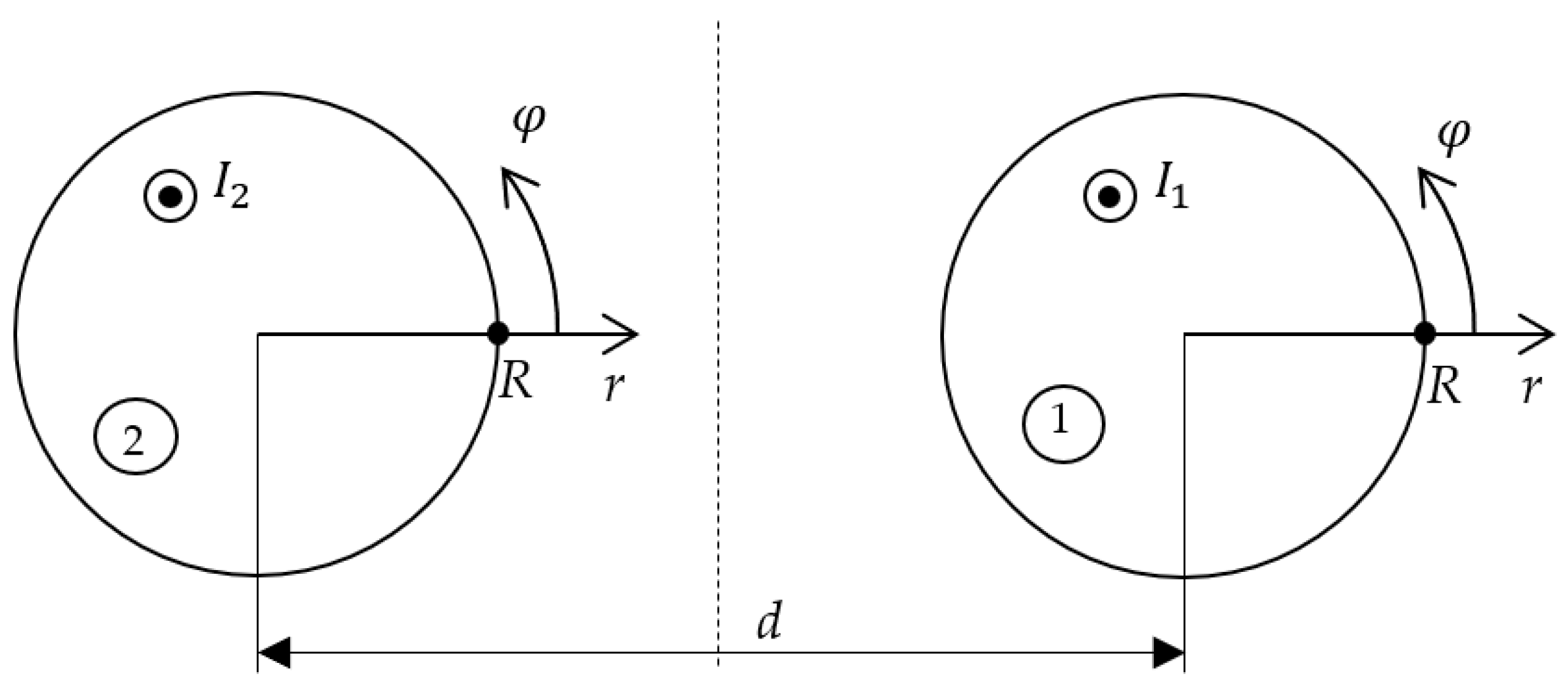
  • Begin from the shape of the conductor (here, two cylindrical conductors of radius R separated by distance d ), material parameters γ and λ , heat transfer coefficient α and the current density in the conductors (here given by Equation (1)).
  • Determine the Green’s function corresponding to the shape and equations describing heat exchange—here given by Equations (3)–(6). Note that Green’s function does not depend on the current density or electrical parameters and is calculated only once—see Equations (8)–(9).
  • Use Equation (7) to determine the temperature at any point in the conductor.
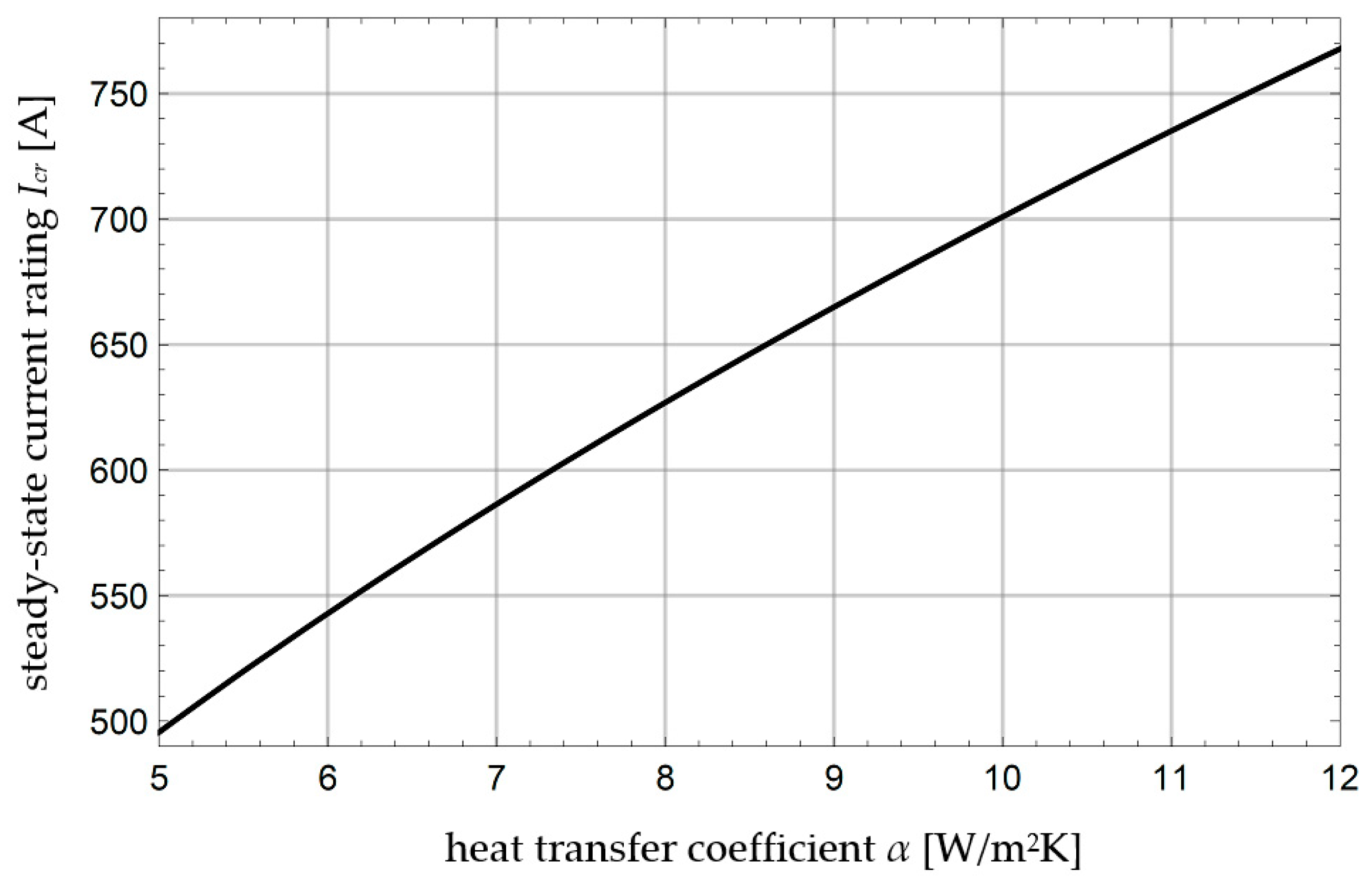
  • Calculate such quantities as the steady-state current rating.

3. Results

3.1. Green’s Function

The Green’s function was determined on the basis of the solution of the above-mentioned auxiliary problem (8)–(9). In order to solve it, expansion into a series of eigenfunctions with respect to the angular coordinate was carried out, and the Dirac delta δ φ θ was represented in the form of a trigonometric series of cosines. A special case for the constant term in the Fourier series was considered separately. As for the radial coordinate, direct integration of Equation (8) was applied taking into account the boundary condition (9) and the properties of the Green’s function (continuity and discontinuity of derivatives at the point ξ , θ ). On the basis of the above, the sought Green’s function was obtained separately for r < ξ and r > ξ as follows:
G r , φ ; ξ , θ = 1 2 π ln ξ R λ α R + n = 1 1 2 n π ξ r R 2 n n λ α R n λ + α R + r ξ n cos n φ θ ,             0 r ξ ,       0 φ , θ < 2 π ,
and
G r , φ ; ξ , θ = 1 2 π ln r R λ α R + n = 1 1 2 n π ξ r R 2 n n λ α R n λ + α R + ξ r n cos n φ θ ,           ξ r R ,     0 φ , θ < 2 π .

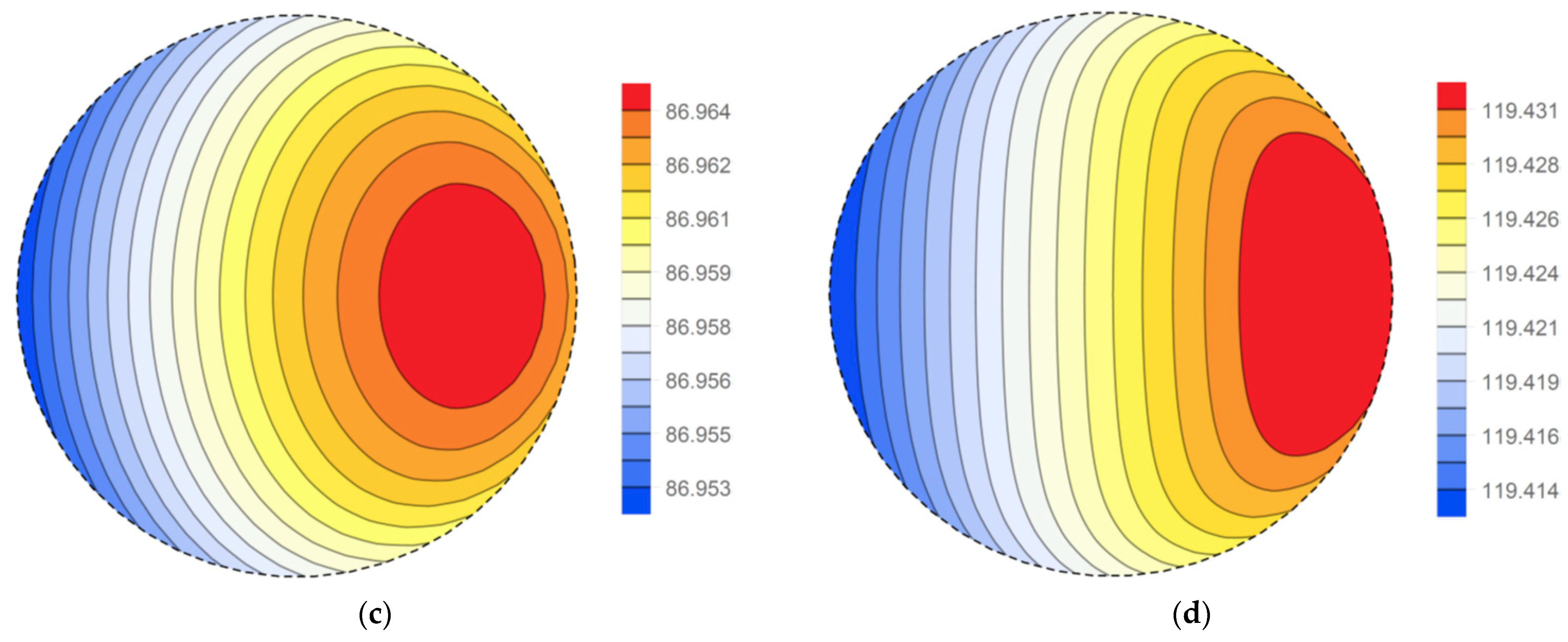
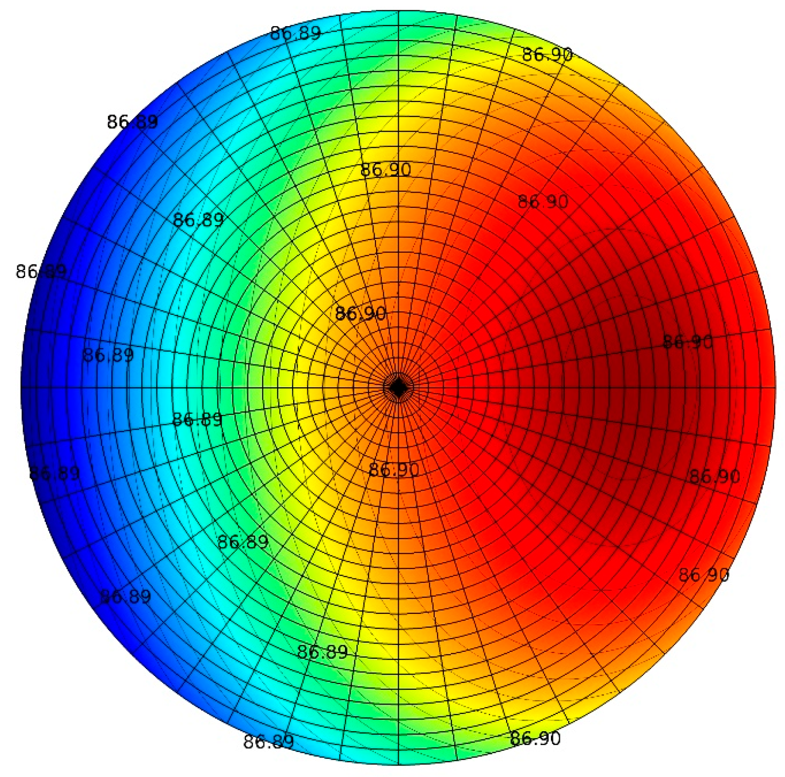
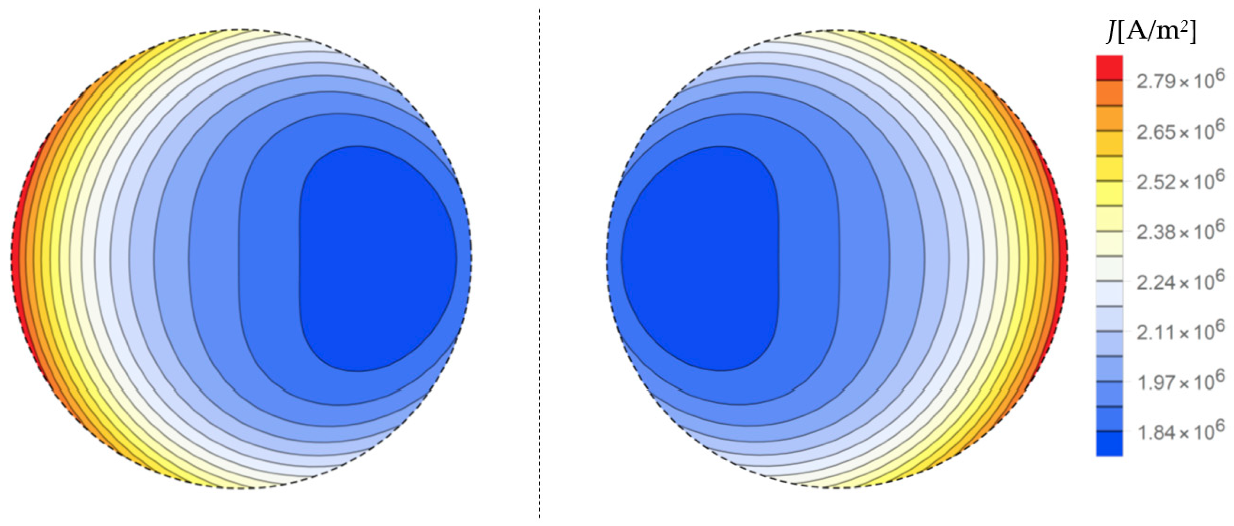
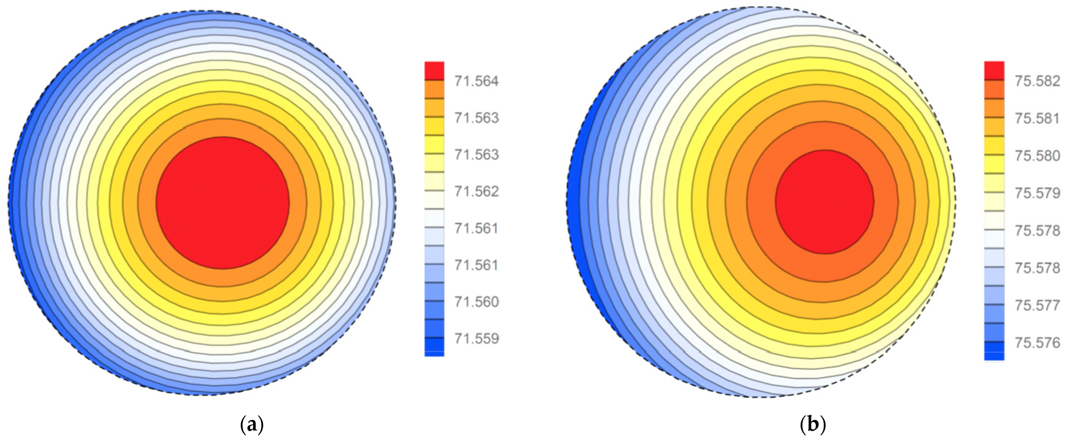
3.2. Temperature Distribution

After using the obtained Green’s function (10)–(11) in Equation (7) and taking into account the previously given definition of temperature increment (3), the sought 2D distribution of the thermal field in the conductor takes the following form:
T r , φ = T 0 + ξ = 0 r θ = 0 2 π g ξ , θ λ 1 2 π ln r R λ α R + n = 1 1 2 n π ξ r R 2 n n λ α R n λ + α R + ξ r n cos n φ θ ξ d ξ d θ + ξ = r R θ = 0 2 π g ξ , θ λ 1 2 π ln ξ R λ α R + n = 1 1 2 n π ξ r R 2 n n λ α R n λ + α R + r ξ n cos n φ θ ξ d ξ d θ ,   0 r R ,         0 φ < 2 π .
Due to the complex form of g ξ , θ , it is impossible to calculate the integrals in (12) analytically for g given by Equations (5) and (1). Nevertheless, Formula (12) may be the basis for obtaining simplified solutions, e.g., by expanding the Bessel functions appearing in (1) into appropriate series [30].
In the case when the proximity effect can be neglected, which occurs for a large enough distance between the wires, function g is independent of the angular coordinate θ . Therefore, integration over θ can be easily performed. As a result, the infinite sum after integration yields zero, and Equation (12) is simplified considerably as follows:
T A C r = T 0 ln r λ 0 r g ξ ξ d ξ + ln R λ + 1 α R 0 R g ξ ξ d ξ 1 λ r R g ξ ξ ln ξ d ξ .
This formula can also be used for direct current, when g ξ , θ = J D C 2 / γ = c o n s t . In such a case, the integrals in Equation (13) can easily be found analytically as follows:
T D C r = T 0 + J D C 2 4 λ γ R 2 r 2 + J D C 2 2 α γ R ,                       0 r R ,
where J D C = I 1 / π R 2 is the direct current density.
A slightly more complicated situation occurs when the skin effect is taken into account. In such a case, after omitting the series related to the proximity effect in Equation (1), it follows that
g ξ = J A C ξ 2 γ = I 1 2 π 2 R 4 Γ R 2 4 γ I 0 Γ ξ I 0 Γ * ξ I 1 Γ R I 1 Γ * R = c I 0 Γ ξ I 0 Γ * ξ .
In the above formula,
c = J D C 2 γ k 2 R 2 2 I 1 Γ R I 1 Γ * R ,
where Γ = 1 + j k , and k = π f μ 0 γ is the reciprocal of the skin depth. Then, integrals of g ξ ξ and g ξ ξ ln ξ with respect to ξ must be evaluated. Since
I 0 Γ ξ I 0 Γ * ξ ξ d ξ = ξ Γ 2 Γ * 2 Γ I 0 Γ * ξ I 1 Γ ξ Γ * I 0 Γ ξ I 1 Γ * ξ ,
it follows that
g ξ ξ d ξ = c 2 ξ 2 W k ξ ,
where the following function W z was introduced for brevity:
W z = 1 z 2 R z 1 + j I 0 1 + j z I 1 1 j z .
The other integral is transformed using partial integration as follows:
g ξ ξ ln ξ d ξ = c 2 ξ 2 W k ξ ln ξ c 2 W k ξ ξ d ξ ,
where Equation (18) was used. The last integral is not elementary; therefore, W z is expanded into a power series, which has the following form:
W z = n = 0 w n z 4 n ,
where
w n = 1 2 n + 1 2 2 n n ! 2 2 n !   = 1 , 1 24 , 1 7680 , ,               n = 0,1 , 2 ,
Then, the integral in Equation (20) becomes
W k ξ ξ d ξ = ξ 2 2 S k ξ .
In the above equation S z is an auxiliary function defined as follows:
S z = n = 0 s n z 4 n ,
where
s n = w n 2 n + 1 = 1 2 n + 1 2 2 2 n n ! 2 2 n !   = 1 , 1 72 , 1 38400 , ,                 n = 0,1 , 2 ,
As a result, the considered integral (20) yields
g ξ ξ ln ξ d ξ = c I 0 Γ ξ I 0 Γ * ξ ln ξ ξ d ξ = c 2 ξ 2 W k ξ ln ξ 1 2 S k ξ .
Equations (18) and (26) are then used in (13). After some transformations, the steady-state temperature takes the following form:
T A C r = T 0 + c 2 α R R 2 W k R + c 4 λ R 2 S k R r 2 S k r .
Taking into account Equation (16), one finally obtains
T A C r = T 0 + J D C 2 γ k 2 R 2 2 I 1 Γ R I 1 Γ * R R 2 α W k R + 1 4 λ R 2 S k R r 2 S k r .
When the skin effect is very weak ( k R 1 ), we have 2 I 1 Γ R I 1 Γ * R k R 2 / 2 , W k R 1 , and S k R 1 , which yields the same expression as for the DC case—see Equation (14).

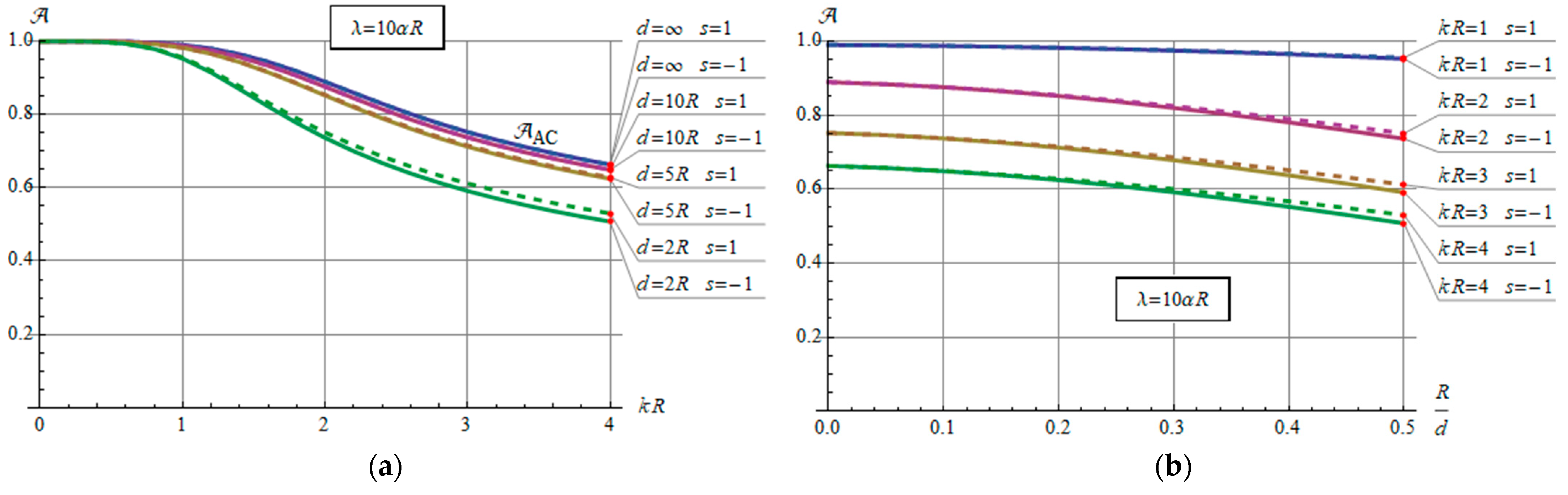
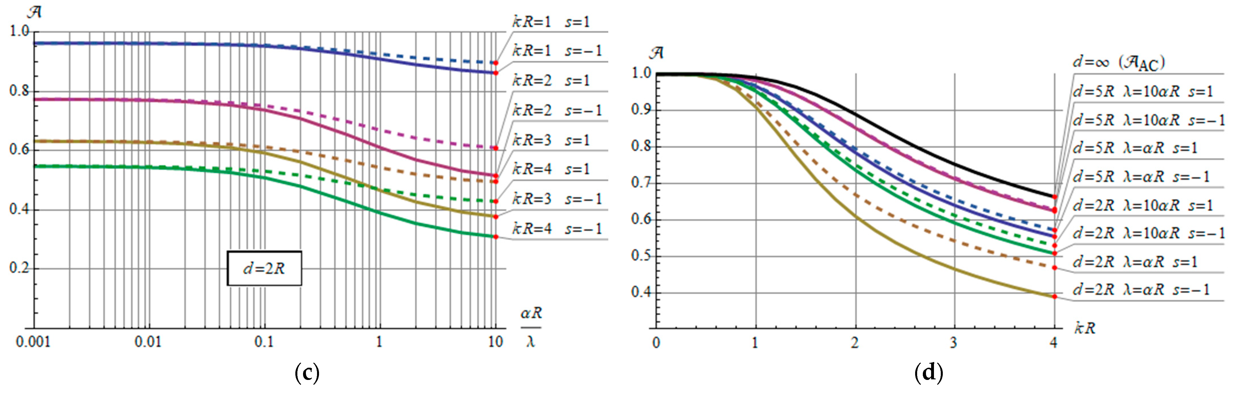
3.3. Temperature on the Conductor’s Surface

When r = R , the second integral in Equation (12) equals zero due to the integration limits; thus, the increase in temperature becomes
ϑ R , φ = 1 2 π ξ = 0 R θ = 0 2 π g ξ , θ 1 α R + 2 n = 1 1 n λ + α R ξ R n cos n φ θ ξ d ξ d θ .
Before dispatching the general case, this integral is considered for the case when the proximity and skin effects are neglected. Equation (14) then yields
ϑ D C R = J D C 2 R 2 α γ = I 1 π R 2 2 R 2 α γ .
A slightly more complicated situation takes place if the skin effect is taken into account (with the proximity effect neglected). In such a case, Equations (13) and (18) can be used to obtain
ϑ A C R = 1 α R 0 R g ξ ξ d ξ = J D C 2 γ R 2 α k 2 R 2 2 I 1 Γ R I 1 Γ * R W k R .
To estimate the influence of the skin effect on the conductor’s temperature (on its surface), the following indicator can be introduced:
T A C k R = ϑ A C R ϑ D C R = R 1 + j k R I 0 1 + j k R 2 I 1 1 + j k R .
This expresses the relative increase in temperature due to the skin effect, illustrated in Figure 3 (blue trace). This expression has the following power series expansion:
T A C k R = 1 + k R 4 48 k R 8 2880 + 11 k R 12 1720320 .
The increase in temperature due to a weak skin effect ( k R 1 ) is below 1/48 (around 2%). On the other hand, the asymptotic expansion for large k R yields
T A C k R 1 2 k R + 1 4 ,                   k R > 2 .
Hence, a strong skin effect contributes to the temperature increase proportionally to k R .
In a similar way, the general case with the proximity effect taken into account is considered. To avoid being distracted by mathematical details, only the final formula is given here, and the derivation is provided in Appendix A. The relative increase in temperature due to skin and proximity effects together is as follows:
T = ϑ ϑ D C = 1 2 l , n = 0 2 b l R a n + l a n * I l , l + n , n cos l φ + l = 0 1 + δ l , 0 b l cos l φ n = 0 l a l n a n * I l , l n , n ,
where δ l , 0 is the Kronecker delta,
a 0 = Γ R 2 1 I 1 Γ R ,                 a n > 0 = s 1 n Γ R R d n 1 I n 1 Γ R ,                 n = 1,2 , 3 ,
b 0 = 1 ,                     b l > 0 = 2 α R l λ + α R ,               l = 1,2 , 3 ,
s = I _ 2 I _ 1 ,
I l , m , n = 0 1 I m Γ R ρ I n Γ * R ρ ρ l + 1 d ρ .
In general, integral (39) must be evaluated numerically, except for special cases, e.g., m = n and l = 0 . Equation (35) reveals that the relative temperature increase is a function of the following dimensionless parameters:
  • the skin effect strength, Γ R = ( 1 + j ) k R ;
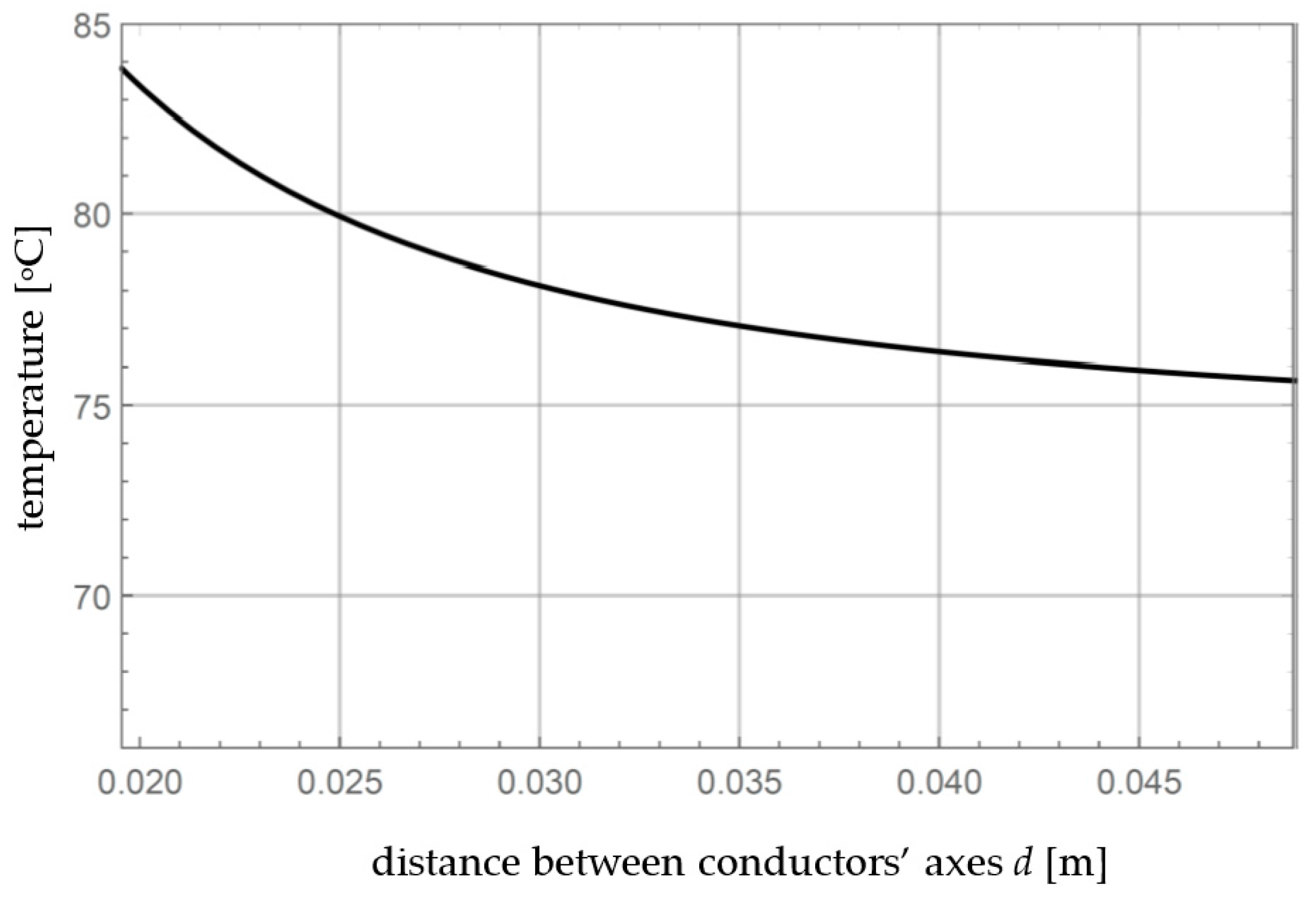
  • the relative distance between the conductors, d / R ;
  • the heat transport ratio, λ / α R ;
  • the direction and modulus of current in the neighboring wire, s (complex number);
  • the observation point on the wire surface (angle φ ).
It is worth noting that the case s = 0 (no current in the neighboring wire) corresponds to neglecting the proximity effect. In such a case, a n = 0 for n > 0 , and Equation (35) simplifies to 2 a 0 a 0 * I 0,0 , 0 , which is the same as (32). Figure 4 shows the influence of various parameters on the relative increase in temperature T .

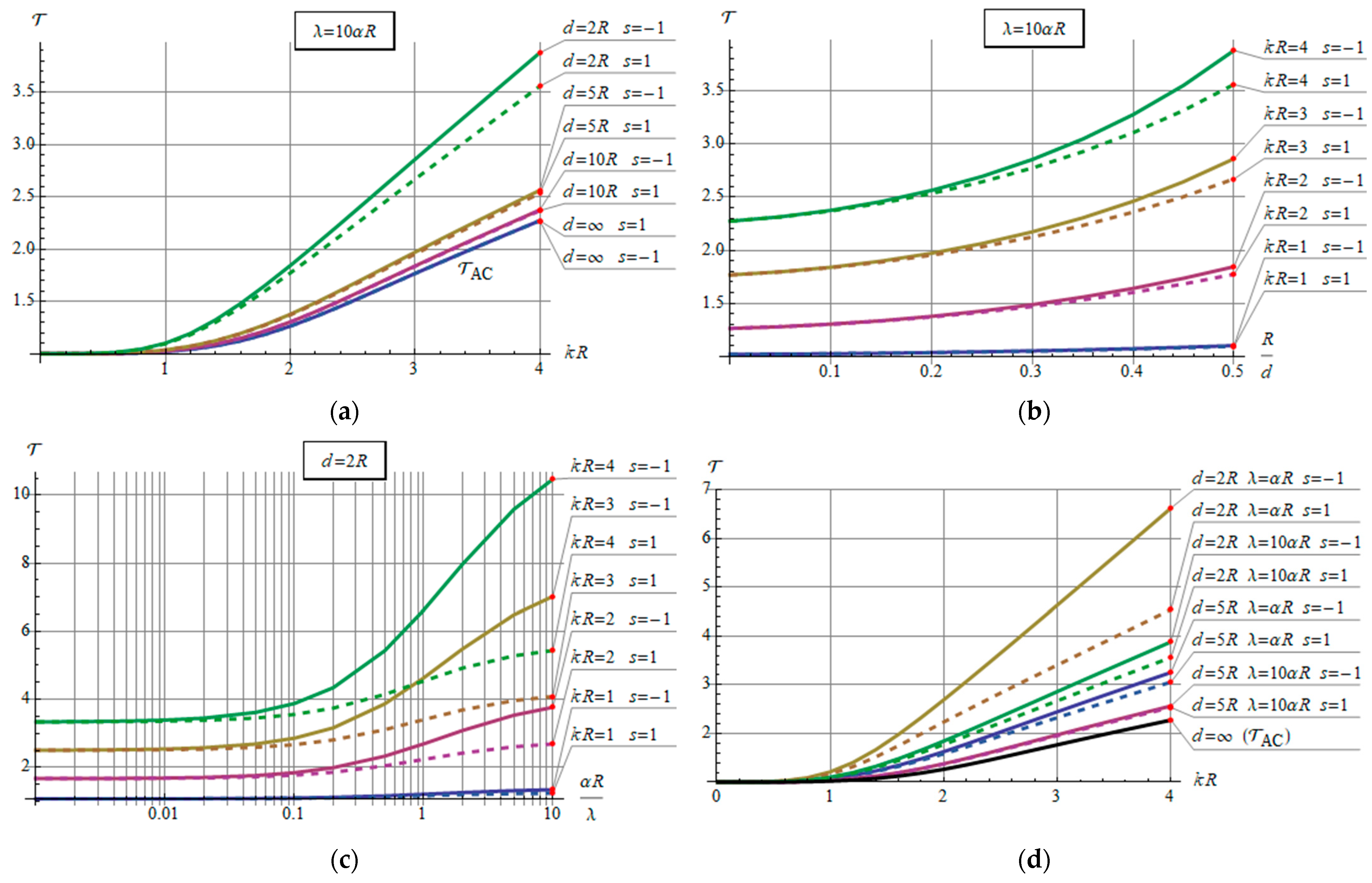
3.4. Steady-State Current Rating of the Conductor

One of the most important indicators of conductors carrying currents is the steady-state current rating. It is limited by the maximum permissible temperature ( T maxp ) to which the conductor can heat up under long-term load conditions. The temperature is usually considered on the conductor’s surface. As a result, the steady-state current rating is determined by solving the following equation with respect to I c r :
max φ T r = R , φ , I c r = T m a x p .
Equation (40) is solved using Equation (29). In general, this requires a numerical approach, but for direct current, Equation (30) can be used to obtain
I c r D C = 2 π 2 α γ R 3 ( T m a x p T 0 ) .
The current rating with skin and proximity effects taken into account can be found using Equations (31) and (40). The result can be expressed as follows:
I c r = A I c r D C ,
where
A = 1 T
is the ampacity ratio representing the influence of skin and proximity effects on the current rating, and T is given by Equation (35) or (32). For s = 0 (when the proximity effect is neglected), it is plotted in Figure 3 (magenta trace). In such a case, the power series expansion for small k R equals
A A C k R = 1 1 96 k R 4 + 31 92160 k R 8 .
The drop in long-term ampacity due to a weak skin effect ( k R 1 ) is below 1/96 (around 1%). In turn, the asymptotic expansion for large k R is as follows:
A A C k R 2 1 + 2 k R ,                   k R > 2 ,
which means that the ampacity drops slowly with an increase in k R . Figure 5 illustrates the effect of various parameters on the value of A .

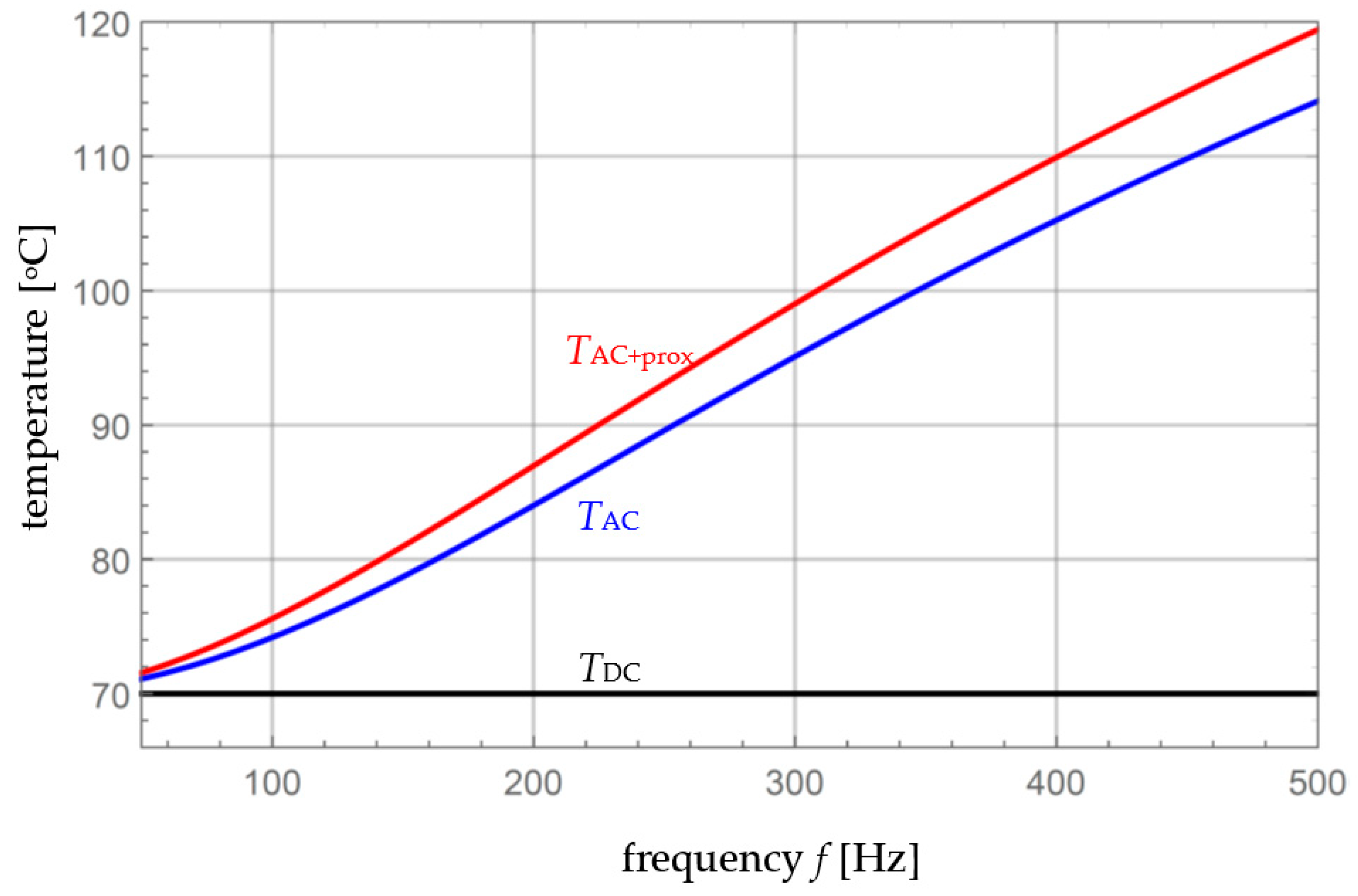
4. Numerical Examples

The developed model was implemented in the Wolfram Mathematica 11.1 environment [31]. The program calculates the distribution of the thermal field using Equation (12) and evaluates the steady-state current rating. The integral expressing the temperature is calculated numerically with the use of methods implemented internally in Wolfram Mathematica. The results of calculations of thermal field distributions using integral (12) are presented graphically. In all numerical examples, a system of two conductors with a cross-sectional area of 300 mm2 was considered. Unless explicitly stated otherwise, the following parameter values were used: R = 0.009772 m, d = 0.05 m, I 1 = I 2 = 595.46 A (same currents), γ = 55 MS/m, f = 50 Hz, T 0 = 20 °C, λ = 360 W/(m⋅K), α = 7 W/m2 K. The DC load I 1   = I 2 = 595.46 A heats the conductor to a temperature of T max = 70 °C. Figure 6 shows the 2D distributions of the thermal field in the cross section of the conductor for the frequencies f = 50, 100, 200 and 500 Hz.
The presented analytical–numerical method was verified by comparing the results with those determined numerically using the finite element method [32,33]. The Heat Transfer module of Comsol Multiphysics software [34] was applied, in which 1000 source elements were used to approximate the heat source distribution g r , φ in the conductor. Numerical calculations were made for a frequency f of 200 Hz. Figure 7 shows the 2D distribution of the thermal field in the conductor obtained in the Comsol Multiphysics program. In order to determine the temperature difference between the calculation results obtained by the analytical–numerical method T a n r , φ and by finite elements T FEM r , φ , the temperature differences T an T FEM at different points of the conductor were examined. Based on the analysis, it was found that the differences did not exceed 0.075 °C at any point in the conductor.
In order to determine the temperature increase caused by the skin and proximity effects, the distributions due to direct current ( T D C ), alternating current with the skin effect but without the proximity effect ( T A C ), and alternating current with both the skin and proximity effects ( T A C + p r o x ) were determined. The results are presented in Figure 8, where temperatures at point r = R and φ = 0 are plotted versus frequency.
One of the fundamental parameters determining the proximity effect is the distance d between the conductors’ axes (Figure 1). Therefore, in Figure 9, the effect of the distance is presented—the temperature at point r = R , φ = 0 versus distance d at a frequency of 100 Hz is plotted (the values of the remaining parameters were the same as those mentioned at the beginning of the section).
From a practical point of view, it is also important to determine the influence of the heat transfer coefficient α on the temperature of the conductors. Due to different cooling conditions or conductor positions, it is difficult to estimate the exact value of this parameter. Therefore, calculations of the conductor temperature were made for the coefficient α varying in the range from 5 to 12 W/m2 K. The temperature at point r = R , φ = 0 versus the heat transfer coefficient α for various frequencies is presented in Figure 10.
The heat transfer coefficient also greatly affects the value of the permissible steady-state current rating of the conductor. Figure 11 presents the dependence of the steady-state current rating on the heat transfer coefficient α for a frequency of 50 Hz. This was obtained based on Equations (43) and (35), where φ was assumed to be 0 in accordance with the results presented in Figure 6, where the maximum temperature on the surface occurs at φ = 0.

5. Discussion

The theoretical considerations show that the skin and proximity effects raise the temperature of the conductors and decrease the ampacity. The skin effect contribution to these quantities was evaluated analytically (Figure 3 and Equations (32) and (43)). It follows that a weak skin effect, when the skin depth is not smaller than the wire radius, increases the incremental temperature T T 0 by up to 2% (Equation (33)) and decreases the ampacity by around 1% compared to the DC case (Equation (44)). However, when the skin depth is at least 2 times smaller than the wire radius, the contribution to an increase in temperature is proportional to the radius/skin depth ratio (Equation (34)). As for ampacity, the drop is approximately inversely proportional to the square root of the aforementioned ratio (Equation (45)).
The influence of the proximity effect on the temperature and steady-state current rating was detected using Equations (35) and (43) and illustrated in Figure 4 and Figure 5. It was shown that the proximity effect contributes to an increase in temperature and a drop in ampacity, both being greater with a smaller distance between the wires (Figure 4a,b,d and Figure 5a,b,d). When the distance between the wires is at least five times the radius and the skin effect is weak, the proximity effect can usually be neglected. The effect of the heat transfer ratio was also shown in Figure 4c and Figure 5c. It follows that for λ / α R > 1000 , the ratio has a negligible effect. Assuming the numerical values given at the beginning of Section 4, it follows that λ / α R > 5000 , so in this case the effect of λ / α R can be neglected.
It is worth noting that the case of opposing currents gives a higher temperature and lower ampacity than the case of the same currents. This is because the maximum current density for opposing currents is larger than that for the same currents (this can be seen when analyzing Equation (1)). Hence, opposing currents generate more heat than the same currents (under the same circumstances).
The temperature distributions in the cylindrical conductor shown in Figure 6 indicate that an increase in frequency has a significant effect on the temperature of the conductor and causes an increase in temperature. The physical reason for this is that the electrical resistance of the cylindrical conductor grows with frequency, which causes more heat to be generated in the conductor. The plots in Figure 6 also show that an increase in frequency causes the temperature maximum to move from the center of the conductor towards the outer sides of the conductors, which is related to the increasing intensity of induced eddy currents. However, the temperature values across the cross section for a given frequency are very close because of the very high thermal conductivity of copper. In the case of opposing currents, the corresponding temperature distributions in each conductor are nearly symmetrical to those shown in Figure 6, but with the maximum shifted towards the left side, which corresponds to the closest points of both conductors (plots not included). However, for the considered values of the parameters, the temperatures are almost identical to those for currents flowing in the same direction.
The temperature distributions obtained using the proposed method and finite elements for a frequency of 200 Hz (Figure 6c and Figure 7) are very close. The temperature differences between the two methods are insignificant and can be attributed to the numerical computations. Thus, the semi-analytical method presented in the paper should be considered verified.
Figure 8 shows that the skin and proximity effects contribute to an increase in temperature, and the higher the frequency, the higher the impact. For example, the approximate temperature increase due to the skin effect is T A C T D C ≈ 1.1 °C at a frequency of 50 Hz, whereas it is around 44.1 °C at a frequency of 500 Hz. Since T D C T 0 ≈ 50 °C in this case, the relative increases are around 2% and 88%, which agrees with the theoretical considerations for T A C and Figure 3. As for the contribution to temperature due to the proximity effect, it equals around T A C + p r o x T A C ≈ 0.46 °C for 50 Hz and 5.3 °C for 500 Hz. It follows that the skin effect has a greater impact on the temperature rise of the conductor than the proximity effect ( T A C T D C > T A C + p r o x T A C ). Moreover, the proximity effect plays an important role only when the conductors are close (Figure 9). At greater distances, i.e., for d > 5 R , the influence of the proximity effect on the temperature of the conductor becomes negligible.
An increase in the heat transfer coefficient has a large influence on the temperature of the conductor (Figure 10). Increasing the value of the heat transfer factor corresponds to higher heat exchange with the environment and significantly reduces the temperature of the conductor. As a result, it is possible to load the conductor with higher current. Also, an increase in the value of the heat transfer coefficient significantly affects the value of the steady-state current rating, enlarging its value with an increase in α (Figure 11).

6. Conclusions

In this paper, a semi-analytical method for determining the distribution of the temperature in two parallel cylindrical conductors, taking into account the skin and proximity effects, was developed. Based on the shape and assumed heat exchange model, the Green’s function was determined. Then, the integral formula for temperature at any point in the conductor can be obtained provided that the current density is known. Unfortunately, the integral cannot be fully evaluated analytically due to the complexity of the integrand for the general case; therefore, a numerical procedure is required at this step. Nevertheless, the obtained integral relationships are the basis for obtaining approximations or simplified solutions for special cases. Although the numerical examples are for the case of the same currents in the conductors, the developed method makes it possible to calculate the thermal field distributions for any currents and for any dimensions of both conductors.
The method presented in this paper also makes it possible to determine other important parameters of the conductors, e.g., the steady-state current rating. The theoretical considerations were applied to evaluate the skin and proximity effects on the conductor’s temperature and steady-state current rating. The skin effect contributions are negligible for skin depths greater than the wire radius. The proximity effect can be neglected when the distance between the wires is greater than around five times the radius and when the skin depth is not smaller than the wire radius.
Although this paper focused on two round conductors, the method can also be used for configurations with more round wires, e.g., three-phase cables. It is worth noting that the Green’s function will remain unchanged in this case. The same methodology can be used for tubular wires or other shapes, provided that the Green’s function can be determined and the current density is known.

Author Contributions

Conceptualization, M.Z., T.S. and P.J.; methodology, M.Z. and P.J.; software, M.Z.; validation, T.S.; formal analysis, M.Z. and P.J.; investigation, M.Z., T.S. and P.J.; resources, M.Z.; data curation, M.Z.; writing—original draft preparation, M.Z.; writing—review and editing, P.J. and T.S.; visualization, M.Z. and P.J.; supervision, P.J. and T.S. All authors have read and agreed to the published version of the manuscript.

Funding

This research was financially supported by the Faculty of Electrical Engineering of the Częstochowa University of Technology and the Faculty of Electrical Engineering of the Technical University of Białystok. This research received no external funding. The APC was partially funded by the Częstochowa University of Technology (BS/PB-3-300-301/11/20/P) and partially covered with vouchers.

Institutional Review Board Statement

Not applicable.

Informed Consent Statement

Not applicable.

Data Availability Statement

Data are available from the corresponding author upon request.

Conflicts of Interest

The authors declare no conflict of interest.

Appendix A. Derivation of Equation (35)

Let us introduce the symbols given by Equations (36)–(38). Then, the current density defined by Equation (1) can be expressed as follows:
J 1 ξ , θ = I 1 π R 2 n = 1 a n I n Γ ξ cos n θ ,
so that the power density given by Equation (5) becomes equal to
g ξ , θ = 1 γ | I 1 |   π R 2 2 m , n = 0 a m a n * I m Γ ξ I n Γ * ξ cos m θ cos n θ .
Using this in Equation (29) yields
ϑ R , φ = 1 2 π 1 α R γ | I 1 |   π R 2 2 m , n , l = 0 C l , m , n D l , m , n ,
where
C l , m , n = 0 2 π cos l φ θ cos m θ cos n θ d θ ,
D l , m , n = ξ = 0 R b l ξ R l a m I m Γ ξ a n * I n Γ * ξ ξ d ξ = b l a m a n * R 2 I l , m , n ,
where I l , m , n is given by Equation (39). Let us consider C l , m , n . Since the integrand is a periodic function with period 2 π , the integration interval can be changed from 0 ,   2 π to π , π . Then, by using the identity cos x y = cos x cos y + sin x sin y , it follows that
C l , m , n = cos l φ π π cos l θ cos m θ cos n θ d θ + sin l φ π π sin l θ cos m θ cos n θ d θ .
The second integral equals zero, because an odd function is being integrated over a symmetric interval. The first integral can be easily calculated:
C l , m , n = 1 2 sin l m n π l m n + sin l + m n π l + m n + sin l m + n π l m + n + sin l + m + n π l + m + n cos l φ .
If none of the denominators in the brackets is zero, then C l , m , n = 0 ; otherwise, a limit of sin x π x as x 0 , which yields π , should be used. As a result, it follows that the expression in the brackets can be 0, π , 2 π or 4 π . More specifically,
  • if l = m = n = 0 , then = 4 π ;
  • if l = m = n > 0 , then = 0 ;
  • if two numbers of l , m , n are equal and greater than zero and the third one equals zero, then = 2 π ;
  • if two numbers of l , m , n are greater than zero and the third one equals their sum, then = π ;
  • otherwise, = 0 .
The above results can be gathered into one formula as follows:
C l , m , n = π 2 δ m , n + l + δ n , m + l + 1 + δ l , 0 δ m , l n cos l φ ,
where δ i , j is the Kronecker delta. Using this in Equation (A3) yields
ϑ R , φ = 1 4 α γ R | I 1 |   π R 2 2 l = 0 n = 0 D l , n + l , n + D l , n , n + l + 1 + δ l , 0 n = 0 l D l , l n , n cos l φ ,
and by using Equation (A5), it follows that
ϑ R , φ = R 2 α γ | I 1 |   π R 2 2 1 2 l = 0 b l n = 0 a n + l a n * I l , n + l , n + a n a n + l * I l , n , n + l + 1 + δ l , 0 n = 0 l a l n a n * I l , l n , n cos l φ .
Since a n a n + l * I l , n , n + l = a n + l a n * I l , n + l , n * , the complex identity z + z * = 2 R z can be used to simplify the expression. Finally, taking into account Equation (30) defining ϑ D C , Equation (35) is thus obtained.

References

  1. Anders, G.J. Rating of Electric Power Cables: Ampacity Computations for Transmission, Distribution and Industrial Application; McGraw-Hill Professional: Columbus, OH, USA, 1997. [Google Scholar]
  2. Morgan, V.T. The current distribution, resistance and internal inductance of linear power system conductors—A review of explicit equations. IEEE Trans. Power Deliv. 2013, 38, 1252–1262. [Google Scholar] [CrossRef]
  3. Popović, Z.; Popović, B.D. Introductory Electromagnetics; Prentice Hall: Hoboken, NJ, USA, 1998. [Google Scholar]
  4. Shazly, J.H.; Mostafa, A.M.; Ibrahim, D.K.; Abo El Zahab, E.E. Thermal analysis of high-voltage cables with several types of insulation for different configuration in the presence of harmonics. IET Gener. Transm. Distrib. 2017, 11, 3439–3448. [Google Scholar] [CrossRef]
  5. Wang, Z.; Zhong, J.; Jiang, J.; Hr, Y.; Wang, Z.; Zhang, H. Development of temperature rise simulation APP for three-phase common enclosure GIS/GIL. In Proceedings of the 5th IEEE Conference on Energy Internet and Energy System Integration, Taiyuan, China, 22–25 October 2021. [Google Scholar]
  6. Szczegielniak, T.; Kusiak, D.; Jabłoński, P. Thermal analysis of the medium voltage cable. Energies 2021, 14, 4164. [Google Scholar] [CrossRef]
  7. Smirnova, L.; Juntunen, R.; Murashko, K.; Musikka, T.; Pyrhönen, J. Thermal analysis of the laminated busbar system of a multilevel converter. IEEE Trans. Power Electron. 2016, 31, 1479–1488. [Google Scholar] [CrossRef]
  8. Li, S.; Han, Y.; Liu, C. Coupled multiphysics field analysis of high-current irregular-shaped busbar. IEEE Trans. Compon. Packag. Manuf. Technol. 2019, 9, 1805–1814. [Google Scholar] [CrossRef]
  9. Chávez, O.; Godínez, F.; Méndez, F.; Aguilar, A. Prediction of temperature profiles and ampacity for a monometallic conductor considering the skin effect and temperature-dependent resistivity. Appl. Therm. Eng. 2016, 109, 401–412. [Google Scholar] [CrossRef]
  10. Levèvre, A.; Miègeville, L.; Fouladgar, J.; Olivier, G. 3-D Computation of transformers overheating under nonlinear loads. IEEE Trans. Magn. 2005, 41, 1564–1567. [Google Scholar] [CrossRef]
  11. Shimotsu, T.; Koike, K.; Kondo, K. Temperature rise estimation of high power transformers of contactless power transfer system considering the influence of skin effect and proximity effect. In Proceedings of the 19th International Conference on Electrical Machines and Systems, ICEMS, Chiba, Japan, 13–16 November 2016. [Google Scholar]
  12. Szczegielniak, T.; Jabłoński, P.; Kusiak, D. Analytical approach to current rating of three-phase power cable with round conductors. Energies 2023, 16, 1821. [Google Scholar] [CrossRef]
  13. Kocot, H.; Kubek, P. The analysis of radial temperature gradient in bare stranded conductors. Przegląd Elektrotechniczny 2017, 10, 132–135. [Google Scholar] [CrossRef]
  14. Zaręba, M.; Gołębiowski, J. The thermal characteristics of ACCR lines as a function of wind speed—An analytical approach. Bull. Pol. Acad. Sci. Tech. Sci. 2022, 70, e141006. [Google Scholar] [CrossRef]
  15. Gołębiowski, J.; Zaręba, M. Analytical modelling of the transient thermal field of a tubular bus in nominal rating. COMPEL Int. J. Comput. Math. Electr. Electron. Eng. 2019, 38, 642–656. [Google Scholar] [CrossRef]
  16. Henke, A.; Frei, S. Fast analytical approaches for the transient axial temperature distribution in single wire cables. IEEE Trans. Ind. Electron. 2022, 69, 4158–4166. [Google Scholar] [CrossRef]
  17. Wang, P.Y.; Ma, H.; Liu, G.; Han, Z.Z.; Guo, D.M.; Xu, T.; Kang, L.Y. Dynamic thermal analysis of high-voltage power cable insulation for cable dynamic thermal rating. IEEE Access 2019, 7, 56095–56106. [Google Scholar] [CrossRef]
  18. Shen, P.; Guo, X.; Fu, M.; Ma, H.; Wang, Y.; Chu, Q. Study on temperature field modeling and operation optimization of soil buried double-circuit cables. In Proceedings of the 20th International Conference on Electrical Machines and Systems (ICEMS), Sydney, Australia, 11–14 August 2017. [Google Scholar] [CrossRef]
  19. Jabłoński, P.; Szczegielniak, T.; Kusiak, D.; Piątek, Z. Analytical-numerical solution for the skin and proximity effect in two parallel round conductors. Energies 2019, 12, 3584. [Google Scholar] [CrossRef]
  20. Lehner, G. Electromagnetic Field Theory; Springer: Heidelberg, Germany, 2010. [Google Scholar]
  21. Riley, K.F.; Hobson, M.P.; Bence, S.J. Mathematical Methods for Physics and Engineering; Cambridge University Press: New York, NY, USA, 2002. [Google Scholar]
  22. Manneback, C. An integral equation for skin effect in parallel conductors. J. Math. Phys. 1922, 1, 123–146. [Google Scholar] [CrossRef]
  23. Dlabač, T.; Filipović, D. Integral equation approach for proximity effect in a two-wire line with round conductors. Tech. Vjesn. 2015, 22, 1065–1068. [Google Scholar] [CrossRef]
  24. Latif, M.J. Heat Conduction; Springer: Haidelberg, Germany, 2009. [Google Scholar]
  25. Hahn, D.W.; Ozisik, M.N. Heat Conduction; John Wiley & Sons: Hoboken, NJ, USA, 2012. [Google Scholar]
  26. Bergman, T.L.; Lavine, A.S.; Incropera, F.P.; Dewitt, D.P. Fundamentals of Heat and Mass Transfer; John Wiley and Sons: Hoboken, NJ, USA, 2011. [Google Scholar]
  27. Cole, K.D.; Beck, J.V.; Haji-Sheikh, A.; Litkouhi, B. Heat Conduction Using Green’s Functions; CRC Press: Boca Raton, FL, USA, 2011. [Google Scholar]
  28. Greenberg, M.D. Applications of Green’s Functions in Science and Engineering; Dover Publications: Mineola, NY, USA, 2015. [Google Scholar]
  29. Duffy, D.G. Green’s Functions with Applications; CRC Press: Boca Raton, FL, USA, 2015. [Google Scholar]
  30. Greenberg, M.D. Advanced Engineering Mathematics; Prentice Hall: Hoboken, NJ, USA, 1988. [Google Scholar]
  31. Wolfram Research Inc. Mathematica; Wolfram Research Inc.: Champaign, IL, USA, 2020. [Google Scholar]
  32. Nithiarasu, P.; Lewis, R.W.; Seetharamu, K.N. Fundamentals of the Finite Element Method for Heat and Mass Transfer; John Wiley and Sons: Chichester, UK, 2016. [Google Scholar]
  33. Brener, S.; Scott, R.L. The Mathematical Theory of Finite Element Method; Springer: Berlin, Germany, 2008. [Google Scholar]
  34. COMSOL Multiphysics, Version 4.3. Documentation for COMSOL Release 4.3. COMSOL: Burlington, MA, USA, 2013.
Figure 1. System of two parallel cylindrical conductors.
Energies 16 06341 g001
Figure 2. Distribution of the current density in the system of the two parallel cylindrical conductors for I 1 = I 2 = 595.46 A (same direction), f = 50 Hz, d = 0.05 m, R = 0.009772 m, and γ = 55 MS/m.
Energies 16 06341 g002
Figure 3. The skin effect’s influence on the temperature ( T A C —thick blue line) and steady-state current rating ( A A C —thick magenta line): dashed lines—power series expansions for small k R ; black solid lines—asymptotic expansions for large k R .
Energies 16 06341 g003
Figure 4. The relative increase in temperature due to the skin and proximity effects (solid lines—opposing currents, dashed lines—same currents): (a) the effect of k R for various distances between the wires; (b) the effect of distance between the wires for various k R ; (c) the effect of the heat transfer ratio for various k R ; (d) the effect of k R for various distances and transfer ratios.
Energies 16 06341 g004
Figure 5. The relative drop in the steady-state current rating due to the skin and proximity effects (solid lines—opposing currents, dashed lines—same currents): (a) the effect of k R for various distances between the wires; (b) the effect of distance between the wires for various k R ; (c) the effect of the heat transfer ratio for various k R ; (d) the effect of k R for various distances and heat transfer ratios.
Energies 16 06341 g005aEnergies 16 06341 g005b
Figure 6. Distribution of the temperature in the cylindrical conductor for frequency f = 50 Hz (a), 100 Hz (b), 200 Hz (c), 500 Hz (d); other parameters given at the beginning of Section 4.
Energies 16 06341 g006aEnergies 16 06341 g006b
Figure 7. The distribution of the temperature obtained by Comsol Multiphysics software in the cylindrical conductor at a frequency of 200 Hz and with parameters given at the beginning of Section 4.
Energies 16 06341 g007
Figure 8. Temperature values at point r = R , φ = 0 versus frequency (parameter values given at the beginning of Section 4): T D C —due to direct current; T A C —due to alternating current with the skin effect but without the proximity effect; T A C + p r o x —due to alternating current with both the skin and proximity effects.
Energies 16 06341 g008
Figure 9. Temperature at point r = R , φ = 0 versus distance d (2 R d ≤ 5 R ) for a frequency of 100 Hz (other parameters given at the beginning of Section 4).
Energies 16 06341 g009
Figure 10. Temperature at point r = R , φ = 0 versus the heat transfer coefficient α for frequencies 50 Hz, 200 Hz and 500 Hz (other parameters given at the beginning of Section 4).
Energies 16 06341 g010
Figure 11. Steady-state current rating of the conductor for the case of skin and proximity effects as a function of the heat transfer coefficient α for a frequency of 50 Hz (other parameters given at the beginning of Section 4).
Energies 16 06341 g011
Disclaimer/Publisher’s Note: The statements, opinions and data contained in all publications are solely those of the individual author(s) and contributor(s) and not of MDPI and/or the editor(s). MDPI and/or the editor(s) disclaim responsibility for any injury to people or property resulting from any ideas, methods, instructions or products referred to in the content.

