Medium-Term Hydrothermal Scheduling of the Infiernillo Reservoir Using Stochastic Dual Dynamic Programming (SDDP): A Case Study in Mexico

Abstract

This article aims to obtain and evaluate medium-term operating policies for the hydrothermal scheduling problem by using the stochastic dual dynamic programming (SDDP) approach. To this end, to feed the mathematical model and build the probability distribution functions that best fit each month of the actual inflow volume, monthly inflow data recorded from 1938 to 2018 for the Infiernillo reservoir located in Mexico were employed. Moreover, we simulated inflow volume scenarios using the Monte Carlo method for each month of a one-year planning period. The SDDP approach to solving the optimization problem consisted of the simulation of one forward scenario per iteration and the stabilization of the total operating cost as a convergence criterion, which results in an operating policy. We then assessed its quality by estimating the one-sided optimality gap. It is worth mentioning that the best operation policy required scenario trees of up to 17,000 inflow realizations per stage. Additionally, to study the evolution of the expected value along the planning horizon of the main variables involved in the medium-term hydrothermal scheduling problem, we simulated the best operation policy over 10,000 inflow scenarios. Finally, to show the practical value of the proposed approach, we report its computational complexity.

1. Introduction

The rapid increase in energy demand around the world (especially in developing countries), amid the interest in making power systems as environmentally friendly as possible and the increasing climate impacts which have escalated in recent years, has raised awareness of the importance of rethinking each country’s energy policies toward a more diversified portfolio of renewable resources (see [1,2]). In particular, Latin America has shown significant investment in renewable energy, surpassing USD 80 billion over the 2010–2015 period [3]. Notably, in 2015, Brazil increased its total renewable energy investment to USD 16.4 billion, which was $40\%$ of the total investment in renewables in all of Latin America. Mexico has been the second highest in promoting clean energy, where renewable energy investment doubled between 2014 and 2015 to reach USD 4 billion [4]. These developments have generated opportunities to benefit from complementarities between renewable energy sources [3], such as the ones existing between large hydropower reservoirs and other renewable energy technologies, taking advantage of the fact that hydropower can come online in less than 2 min, which allows the system to cope with renewable resources’ intermittence and their associated forecasting errors (see [5]). In the same sense, in countries with installed pumped-storage hydropower capacity, excess renewable power can be employed to pump water up to the upper reservoir, which has been an efficient strategy to provide ancillary services in order to maintain the generation/demand balance [6]. Moreover, pumped-storage hydropower can add even more flexibility to hydropower plants because of its ability to come online within 75 to 110 s [7]. Furthermore, since several countries have deregulated their electricity markets, grid operators face new challenges while performing power system operation, which is why more flexible power generation is increasingly required to cope with the uncertainty that characterizes electrical systems [8]. Even though hydropower generation represents a small part of Mexico’s electricity generation mix (natural gas, $59.8\%$; coal, $11\%$; oil, $10.2\%$; hydro, $10\%$; nuclear, $3.8\%$; wind, $2.6\%$; geothermal, $2\%$; biofuels and waste, $0.5\%$; solar, $0.1\%$; see [9]), considering stochastic modeling while solving the medium-term hydrothermal scheduling problem (MTHS) is imperative from both economic and operations perspectives. The former could imply millions of dollars (USD) in savings, as shown by the Brazilian experience where, in [10], the economic benefits that resulted from estimating the long-term optimal operating policy using a stochastic model and those obtained using two deterministic models showed that the system operation cost with the stochastic model was tens of millions of dollars (USD) smaller. On a national level, although the MTHS problem in Mexico has not been solved using a stochastic approach, in 2013 the National Center for Energy Control (CENACE), Mexico’s power system operator, updated its short-term hydrothermal coordination planning tool, resulting in savings of USD $2.2$ million from 2013 to 2014 (see [11]). Officially, the deterministic approach has been employed in Mexico to solve the MTHS problem. Although this approach is the basis for the stochastic programming approach, its main drawback is that it does not model the stochastic nature of the problem due to its assumption that only one scenario will occur [12]; therefore, through this approach, it is not possible to obtain a decision that considers the other possible scenarios that can also happen, and one can only obtain a decision that is optimal for a particular realization [13]. Given the stochastic nature of the MTHS problem, it is essential to consider this ingredient in the optimization model in order to obtain more accurate solutions and reduce the expected total cost. One alternative strategy to achieve the aforementioned is to use stochastic programming because it allows one to model the random variables using their probability distribution functions, as estimated from historical data. Since adding all the random variables into a single optimization model may be impractical, given that one of the most relevant challenges in stochastic programming is related to reducing the required runtime to solve a given large-scale optimization problem [14], we only consider inflows as random variables. The stochastic programming approach, i.e., algorithms based on stochastic dynamic programming (SDP) and stochastic dual dynamic programming (SDDP), has been widely applied to estimate the optimal operation of hydrothermal power systems. The first algorithm was officially implemented in Brazil in 1978 [15]. Meanwhile, the SDDP algorithm has raised several concerns that motivate the transition towards a stochastic approach to solve the Mexican medium-term hydrothermal scheduling problem and that contribute to developing mathematical models that lead to better decision-making. In [16], the authors proposed the deterministic dual dynamic programming algorithm to solve an instance within the Brazilian MTHS problem. Ref. [17] implemented the stochastic dynamic programming–convex hull algorithm to solve the long-term operation planning of the Brazilian electrical system, where the inflow energy scenarios were generated by the Periodic Autoregressive Model (PAR(p)). Ref. [18] presented a new approach for scenario tree generation to deal with nonlinearities that generate non-convexity issues which affect the Brazilian long-term operation planning model. On the other hand, ref. [19] estimated the savings obtained by the Brazilian National Plan for Energy Efficiency by analyzing an operating policy that avoided the construction of additional power plants. Moreover, they computed the operational marginal cost through the SDDP algorithm after including stochastic energy efficiencies in the electricity demand. Based on a new scheme to analyze the effects of time-inconsistent policies induced by modeling simplifications in transmission lines and security criteria, ref. [20] solved the long-term hydrothermal operation planning problem using the SDDP algorithm. To assess the impact of different modeling approaches on the long-term operation planning of a hydrothermal power system, ref. [21] built an open-source tool based on an SDDP algorithm. In [22], a model for joint dynamic chance constraints was proposed and applied to an optimization problem in water reservoir management. For a cascaded reservoir optimization problem with uncertainty in inflows, the authors in [23] propose a joint chance-constrained program where uncertainty is described by a causal time series model integrating a persistency effect. Ref. [24] implemented SDDP to solve multistage stochastic programming problems that minimize dynamic coherent risk measures. Regarding the present paper, for the evaluation of the solution quality of the Mexican medium-term hydrothermal scheduling problem, we follow the approach proposed in [25,26,27]; however, we model inflows by the probability distribution functions that best fit each month of the historical record. The SDDP algorithm reaches its convergence when the total operative cost does not vary with additional iterations. Then, we obtain the operating policy, the quality of which depends on the optimality gap. The remainder of this paper is organized as follows: Section 2 presents the motivation for the stochastic programming approach. Section 3 describes the scenario tree construction, the SDDP algorithm and the estimation of the optimality gap. Section 4 presents the main results, from the fitting process of the probability distribution functions to the computational complexity estimation. Finally, Section 5 shows the principal conclusions.

Objective and Motivation

The medium-term hydrothermal scheduling problem aims to obtain the system operating policy to set the dispatch levels of thermal plants and water releases of hydropower plants, which minimizes the expected value of the system operating cost for a planning period of up to 36 months. To motivate our research problem, we highlight the main characteristics of the MTHS problem as follows:

• The MTHS problem is intrinsically stochastic because the variables involved cannot be accurately forecasted (see [14]).
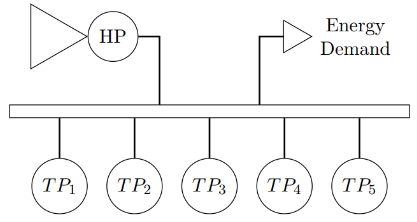
• Given that system reservoirs can transfer energy from one time period to another (it may be from hours to even years ahead, depending on the physical characteristics of the reservoir), the problem is coupled in time. Because of this characteristic, before making decisions regarding the quantity of water to use to produce electric energy, we need to estimate the economic consequences of those decisions. Figure 1 displays a representation of the decision process in hydrothermal systems; it shows that operating decisions influence future operating costs. For example, if reservoirs are depleted in the present and low inflows occur in the future, more thermal generation will be needed to supply energy demand, which will increase the system’s operating cost (or even imply an energy shortage if thermal installed capacity is not sufficient to supply demand). On the other hand, if reservoir levels are kept high in the present through a more intensive use of thermal resources and high inflows occur in the future, the reservoirs’ storage capacities may be exceeded and there will be spillages in the system, increasing the risk of flooding for riparian communities settled downstream the reservoirs. Additionally, the spilled water represents wasted energy (see [28,29]).
• It is a nonlinear optimization problem because of the thermal cost functions and the hydroelectric production functions [30]. However, since the hydrothermal scheduling problem is too complex to be solved by a single optimization model, it is usually decomposed into a chain of subproblems with different planning horizons and degrees of detail in the system representation. Given that this work is focused on a medium-term planning horizon (up to 3 years for the Mexican power system), these functions are approximated by a linear model in order to put greater emphasis on modeling the uncertain nature of the MTHS problem.
• It is a large-scale problem because the number of scenarios grows exponentially with the number of stages [13].

Since the hydrothermal scheduling problem is coupled in time, before making present decisions it is therefore necessary to estimate their future consequences. For this reason, the total operating cost is made up of two costs, the cost associated with present decisions and that related to the future consequences of those decisions. In [19], the authors show the relationship between these costs by presenting three cost functions. The first is the immediate cost function (ICF), which is related to the thermal generation cost required to supply the load and depends on the water stored in a reservoir at the end of a given stage in the following way: if the system operator decides to supply the load with hydropower generation, the stored water is going to be low and the immediate cost will be small given that expensive thermal generation resources are not considered. On the other hand, if the stored water is kept high, the immediate cost increases. The second is the future cost function (FCF), which is related to the expected thermal generation cost that will be incurred in the future (from the next time period to the end of the planning horizon) considering the stored water at the end of the current stage and the future inflows. In this case, if hydro resources are employed in the present, the future cost will increase because there will be no stored water available and the system operator will have to resort to thermal resources to supply the load; conversely, if the reservoir level is kept high in the present, the future cost will be low. Accordingly, the objective of the hydrothermal scheduling problem is to determine the optimal use of water—that is to say, the stored volume at the end of each stage that minimizes the third function, which represents the total cost function (TCF).

2. Deterministic HTS versus Stochastic HTS

Based on an illustrative MTHS problem, this section aims to present the motivation for stochastic modeling and show the economic benefits of its implementation. We consider a two-month planning horizon in which the objective is to supply a constant demand of 1000 MWh. The test system is displayed in Figure 2, and is composed of five thermal power plants and one hydropower plant; the data associated with the power plants are presented in

Table 1. Power plant data.

Thermal Power Plants			Hydropower Plant
Plant	Incr. Cost USD/(MWh)	Inst. Cap. (MW)	Ini. Vol. (Mm${}^{\mathbf{3}}$)	Min. Vol. (Mm${}^{\mathbf{3}}$)	Max. Vol. (Mm${}^{\mathbf{3}}$)	Max. Turb. Outflow (m${}^{\mathbf{3}}$/s)	Productivity Factor (MWh/(m${}^{\mathbf{3}}$/s))
1	10	100
2	20	150
3	40	200	3000	2250	6053.75	1300	0.96
4	80	250
5	500	1000

. First, we consider the deterministic approach, and then we include the stochastic nature of the MTHS in the optimization model.

Regarding the optimization model, a relevant ingredient is given by the hydroelectric production function, which states that the energy generated by a hydropower plant is obtained by a nonlinear function (see [31]). However, in the present paper, the hydro generation is given by the product of the plant productivity factor and the turbined outflow, as can be appreciated in the power balance equation. Accordingly, the deterministic model adapted from [27] is presented below. It is important to recall that in this case we do not consider load shedding, given that the installed capacity of the Mexican thermal system is sufficient to supply the energy demand.

$$\begin{array}{cc}\min \hfill & \sum _{t=1}^T\sum _{j=1}^J{c}_j{\tilde{p}}_{tj}\hfill \end{array}$$

(1)

$$\begin{array}{cc}\hfill \hspace{1em}\hspace{1em}\hspace{1em}\hspace{1em}\hspace{1em}\hspace{1em}\mathrm{s}.\mathrm{t}.:& \sum _{j=1}^J{\tilde{p}}_{tj}+\rho q_t=E_t,\left({\pi }_t^{{}^{\prime }}\right)\forall t\hfill \end{array}$$

(2)

$$\begin{array}{cc}\hfill & v_t=v_{t-1}+b_t-c_0(q_t+s_t),\left({\pi }_t^{{}^{″}}\right)\forall t\hfill \end{array}$$

(3)

$$\begin{array}{cc}\hfill & 0\le {\tilde{p}}_{tj}\le {\tilde{p}}_{jMax}\forall t,j\hfill \end{array}$$

(4)

$$\begin{array}{cc}\hfill & v_{Min}\le v_t\le v_{Max},0\le q_t\le q_{Max},0\le s_t\forall t\hfill \end{array}$$

(5)

The objective function (1) aims to minimize the total operating cost, constraint (2) represents the power balance equations and (3) refers to the stream-flow balance equations. The dual variable of constraint (2) is known as the marginal cost of operation $\left({\pi }_t^{{}^{\prime }}\right)$ and indicates the increase in the operating cost given by a 1 MWh increase in the demand; furthermore, the dual variable of constraint (3) is referred to as the marginal cost of water $\left({\pi }_t^{{}^{″}}\right)$ and represents the decrease in the operating cost due to an increment in hydro generation. On the other hand, the fact that the inflows to the reservoir are random variables raises the following concern: which inflow values should be considered for the first and second stages? Given that decisions must be taken at the present, it is commonly assumed that the first stage inflow can be accurately forecasted, while the second stage inflows are described by a finite set of scenarios with known probabilities (see [32]). The aforementioned is illustrated in Figure 3, where there is a scenario tree with three inflow scenarios in the second stage. In order to answer the previous question first, let us analyze one scenario at a time to determine the associated cost. Under the optimistic scenario, the total operating cost is USD 41,365.48, and the related results are shown in

Table 2. Optimistic scenario results.

Parameter	Stage 1	Stage 2
Operating Cost (USD)	29,954.96	11,410.52
TP${}_1$ (MWh)	100	100
TP${}_2$ (MWh)	150	150
TP${}_3$ (MWh)	200	185.26
TP${}_4$ (MWh)	224.44	0
TP${}_5$ (MWh)	0	0
HP (MWh)	325.56	564.74
Initial Volume (Mm${}^3$)	3000	2250
Inflow (Mm${}^3$)	129.02	1524.79
Turbined Outflow (m${}^3$/s)	339.13	588.27
Spilled Outflow (m${}^3$/s)	0	0
Final Volume (Mm${}^3$)	2250	2250

.

Considering the expected scenario, the total operating cost is USD 160,874.07; in this case, because the inflow during the second stage is lower it is necessary to consider the generation of thermal plants 4 and 5, which increases the second stage cost and consequently the total operating cost.

Table 3. Expected scenario results.

Parameter	Stage 1	Stage 2
Operating Cost (USD)	32,000	128,874.07
TP${}_1$ (MWh)	100	100
TP${}_2$ (MWh)	150	150
TP${}_3$ (MWh)	200	200
TP${}_4$ (MWh)	250	250
TP${}_5$ (MWh)	0	193.75
HP (MWh)	300	106.25
Initial Volume (Mm${}^3$)	3000	2319.02
Inflow (Mm${}^3$)	129.02	217.86
Turbined Outflow (m${}^3$/s)	312.50	110.68
Spilled Outflow (m${}^3$/s)	0	0
Final Volume (Mm${}^3$)	2319.02	2250

shows the corresponding results.

Finally, considering the pessimistic scenario, the total operating cost is USD 194,231.48, which is even higher because the generation of thermal plant 5 is higher during the second stage.

Table 4. Pessimistic scenario results.

Parameter	Stage 1	Stage 2
Operating Cost (USD)	32,000	162,231.48
TP${}_1$ (MWh)	100	100
TP${}_2$ (MWh)	150	150
TP${}_3$ (MWh)	200	200
TP${}_4$ (MWh)	250	250
TP${}_5$ (MWh)	0	260.46
HP (MWh)	300	39.54
Initial Volume (Mm${}^3$)	3000	2319.02
Inflow (Mm${}^3$)	129.02	37.73
Turbined Outflow (m${}^3$/s)	312.50	41.18
Spilled Outflow (m${}^3$/s)	0	0
Final Volume (Mm${}^3$)	2319.02	2250

displays the associated results.

We can appreciate in

Table 5. Total operating costs of the deterministic approach.

Case	Total Operating Cost (USD)
Optimistic scenario	41,365.48
Expected scenario	160,874.07
Pessimistic scenario	194,231.48

that the total operating cost goes from USD 41,365.48 to USD 194,231.48; despite the economic difference, each solution is optimal for its particular scenario. From this perspective, there are two important questions. The first question is regarding which inflow value should be considered for the second stage. The second question is which decision should be taken at the first stage such that the stochasticity in the inflows during the second stage can be considered. As previously mentioned, in the deterministic approach only one scenario is considered at a time. This represents the main drawback of this approach given that regardless of which one is selected it is possible to be certain that it will not occur in the future. This is because the historical record represents only one realization of the inflow’s stochastic process, and therefore a scenario recorded in the past will not repeat itself.

Additionally, although an optimal solution exists for a particular scenario, it is not possible to obtain a robust solution that neutralizes the impacts of the multiple scenarios that can occur (see [33]).

Stochastic HTS

This section provides the results associated with the stochastic programming approach, considering the most likely scenarios explicitly in the mathematical model. Therefore, we describe the corresponding optimization model in its extensive form as follows [27] (for more details about stochastic programming modeling, see [34]):

$$\begin{array}{ccc}\hfill & \min \hfill & \sum _{j=1}^J{c}_j{\tilde{p}}_{1j}^1+\frac{1}{N}\sum _{\omega =1}^N\sum _{j=1}^J{c}_j{\tilde{p}}_{2j}^{\omega }\hfill \end{array}$$

(6)

$$\begin{array}{cc}\hfill s.\mathrm{t}.:& \sum _{j=1}^J{\tilde{p}}_{1j}^1+\rho q_1^1=E_1\hfill \end{array}$$

(7)

$$\begin{array}{cc}\hfill & v_1^1=v_i+b_1^1-c_0(q_1^1+s_1^1)\hfill \end{array}$$

(8)

$$\begin{array}{cc}\hfill & \sum _{j=1}^J{\tilde{p}}_{2j}^{\omega }+\rho q_2^{\omega }=E_2\forall \omega \hfill \end{array}$$

(9)

$$\begin{array}{cc}\hfill & v_2^{\omega }=v_1^1+b_2^{\omega }-c_0(q_2^{\omega }+s_2^{\omega })\forall \omega \hfill \end{array}$$

(10)

$$\begin{array}{cc}\hfill & 0\le {\tilde{p}}_{tj}^{\omega }\le {\tilde{p}}_{jMax}\forall t,j,\omega \hfill \end{array}$$

(11)

$$\begin{array}{cc}\hfill & v_{Min}\le v_t^{\omega }\le v_{Max},0\le q_t^{\omega }\le q_{Max},0\le s_t^{\omega }\forall t,\omega \hfill \end{array}$$

(12)

Unlike the deterministic case, the objective function (6) aims to minimize the sum of the first stage operating cost and the expected value of the second stage cost. For the sake of simplicity, we consider only three inflow scenarios, i.e., $N=3$ as Figure 3 shows. The set of constraints is composed of those related to the first stage (7)–(8) and those associated with each possible inflow scenario (9)–(12). Then,

Table 6. Stochastic approach results.

Variable	Stage 1	Stage 2
		Optimistic	Expected	Pessimistic
		Scenario	Scenario	Scenario
Operating Cost (USD)	32,000	10,388	128,874.07	162,231.48
TP${}_1$ (MWh)	100	100	100	100
TP${}_2$ (MWh)	150	150	150	150
TP${}_3$ (MWh)	200	159.70	200	200
TP${}_4$ (MWh)	250	0	250	250
TP${}_5$ (MWh)	0	0	193.75	260.46
HP (MWh)	300	590.30	106.25	39.54
Initial Volume (Mm${}^3$)	3000	2319.02	2319.02	2319.02
Inflow (Mm${}^3$)	129.02	1524.79	217.86	37.73
Turbined Outflow (m${}^3$/s)	312.50	614.90	110.68	41.18
Spilled Outflow (m${}^3$/s)	0	0	0	0
Final Volume (Mm${}^3$)	2319.02	2250	2250	2250

shows the optimal solution of the different variables involved in the problem.

In the stochastic model, the expected total operating cost equals USD 132,497.85 regardless of which resulting scenario materializes. Even though this cost is not as economical as the one obtained in the optimistic scenario case, there is no certainty that this scenario will occur. On the other hand, through this example we can observe that the size of the problem increases in comparison with the deterministic formulation because in the stochastic approach we have a set of constraints for each node of the scenario tree, which may also increase the computation time. It is worth mentioning that by increasing the number of scenarios, hopes for solving the resulting optimization problem based on linear programming solvers are quickly dismissed in favor of specialized solution algorithms [33], particularly those based on decomposition techniques and sampling.

3. Mathematical Modeling

This section presents the background necessary to solve the MTHS problem and to perform the solution quality evaluation, so we first introduce the scenario tree generation.

3.1. Scenario Tree Generation

According to [25], a T-stage stochastic linear program with recourse is represented as follows:

$$\begin{array}{cc}\hfill z^{*}=\min & c_1{x}_1+\mathbb{E}\left[h(x_1,b_2)\right]\hfill \\ \hfill \mathrm{s}.\mathrm{t}.:& A_1{x}_1=B_1{x}_0+b_1\hfill \\ \hfill & x_1\ge 0\hfill \end{array}$$

(13)

where, for stages $t=2,\dots ,T$, we have

$$\begin{array}{cc}\hfill h_t(x_{t-1},b_t)=\min & c_t{x}_t+\mathbb{E}\left[h_{t+1}(x_t,b_{t+1})\right]\hfill \\ \hfill \mathrm{s}.\mathrm{t}.:& A_t{x}_t=B_t{x}_{t-1}+b_t\hfill \\ \hfill & x_t\ge 0\hfill \end{array}$$

(14)

For $t=1,2,\dots ,T$, the matrix $A_t$ has $m_t$ rows and $d_t$ columns. Meanwhile, the dimensions of the remaining vectors and matrices depend on those of $A_t$. The random parameters in the model (13)–(14) correspond to inflow volumes to the reservoirs represented by $b_t$. Moreover, the stochastic process governing the inflows is one of the most important characteristics of the medium-term/long-term hydrothermal scheduling problem. One way to represent how these variables may evolve over the planning period is through a scenario tree. We denote a realization of the random vector $b_t$ by $b_t^{{\omega }_t}$, and when $b_t$ is a continuous random variable we build a finite scenario tree by sampling; for more details, we refer the reader to [25]. Figure 4 is adapted from [25] and displays an example of a three-stage scenario tree with common samples (in this case, we assume that vectors $b_t,t=2,\dots ,T$ are interstage independent). This characteristic of the scenario tree makes it possible to add Benders’ cut generated for a particular scenario to all the nodes in same stage, which is known as cut sharing (see [35]) and is an important characteristic of the SDDP algorithm as described in [30].

3.2. Stochastic Dual Dynamic Programming Algorithm

The SDDP algorithm proposed in [28] is designed to cope with the curse of dimensionality associated with the SDP approach when estimating future cost functions. The SDDP algorithm has two main steps, known as forward and backward simulations. In the forward one, we first sample a set of forward scenarios to simulate the operation of the system reservoir along the planning horizon. In the backward simulation, we add cuts to the set that defines the current approximation of the future cost functions considering as initial conditions the final volumes obtained in the forward simulation (see [16,28]). For the optimization model solved at each stage (15)–(18), $G_t$ and $g_t$ represent the cut-gradient matrix and the cut-intercept vector for stage t computed during the running of the SDDP algorithm; additionally, each backward simulation of the SDDP along a forward scenario increases $G_t$ and $g_t$ with one additional row. The optimization problem solved at stage t is represented as follows [25,26]:

$$\begin{array}{cc}\hfill z_t=\min & c_t{x}_t+{\theta }_t\hfill \end{array}$$

(15)

$$\begin{array}{ccc}\hfill & \mathrm{s}.\mathrm{t}.:\hfill & A_t{x}_t=B_t{x}_{t-1}+b_t:{\pi }_t\hfill \end{array}$$

(16)

$$\begin{array}{cc}\hfill & -G_t{x}_t+e{\theta }_t\ge g_t\hfill \end{array}$$

(17)

$$\begin{array}{cc}\hfill & x_t\ge 0\hfill \end{array}$$

(18)

From (15), ${\theta }_t$ in the objective function coupled with constraint (17) represents an outer linearization of the recourse function $\mathbb{E}\left[h_{t+1}(x_t,b_{t+1})\right]$ displayed in (14). For the optimization problem solved at stage T these terms are absent, given than the FCF for that stage is zero. Additionally, ${\pi }_t$ denotes the dual vector associated with constraints (16) and e is a unit vector. By adding ${\omega }_t$ superscripts to the optimal value $\left(z_t^{{\omega }_t}\right)$ and to the primal $\left(x_t^{{\omega }_t},{\theta }_t^{{\omega }_t}\right)$ and dual solutions $\left({\pi }_t^{{\omega }_t}\right)$ we refer to model (15)–(18) as sub(${\omega }_t$). Moreover, considering the same stopping criterion employed when the SDDP was first conceived, the algorithm converges when the first stage total operating cost at iteration k$\left({\underline{z}}^k\right)$ belongs to a confidence interval given by (see [25,26,28]):

$$\left({\overline{z}}^k-1.96\frac{{\sigma }_z}{\sqrt{N}},{\overline{z}}^k+1.96\frac{{\sigma }_z}{\sqrt{N}}\right).$$

(19)

In (19), we have that:

$${\overline{z}}^k=c_1{x}_1^k+\frac{1}{N}\sum _{\omega =1}^N\sum _{t=2}^T{c}_t{\left[x_t^{{\omega }_t}\right]}^k$$

(20)

$${\sigma }_z=\sqrt{\frac{1}{N-1}\sum _{\omega =1}^N{\left({\overline{z}}^{\omega }-{\overline{z}}^k\right)}^2}$$

(21)

and ${\overline{z}}^{\omega }$ represents the immediate cost of scenario $\omega$, defined by:

$${\overline{z}}^{\omega }=c_1{x}_1^k+\sum _{t=2}^T{c}_t{\left(x_t^{{\omega }_t}\right)}^k$$

(22)

The convergence criterion proposed in [28] has some particularities that were studied in [36,37], which depends on the number of scenarios sampled in the forward simulation and the confidence level considered while building the confidence interval. On the other hand, different proposals for convergence criteria published in the literature consider a sample of 200 scenarios during the forward simulation (see [24,38,39]). In the present work, and according to the research developed in [40,41], only one forward scenario is considered. In view of the above, the stabilization of the first stage total operating cost is the convergence criterion. Hence, at iteration k, we perform a forward and a backward simulation. Meanwhile, with the first stage total operating cost ${\underline{z}}^k$ obtained at the end of that iteration, we compute the following ratio [42]:

$${\beta }^k=\frac{{\underline{z}}^k-{\underline{z}}^{k-1}}{{\underline{z}}^k}$$

(23)

We consider that the algorithm converges when ${\beta }^k$ is lower than a given tolerance $ϵ$ for the last 10 iterations. Once the stopping criterion is satisfied, we display the following results: (i) Set of cuts: $G_t$ and $g_t$, $t=1,\dots ,T$. (ii) First stage solution: $x_1=x_1^k$. (iii) Lower bound on the optimal solution: $\underline{z}={\underline{z}}^k$.

Remark 1. 

The system operating policy is one of the main results of the MTHS problem because by this policy it is possible to determine dispatch decisions for each stage of the planning period and each inflow scenario. Then, once the algorithm converges, it is crucial to evaluate how good the obtained operating policy is to determine the size of the scenario tree, from which it is possible to obtain a good trade-off between the solution quality and the computational effort required to solve the associated problem.

3.3. Solution Quality Evaluation

Consider the policy approximated by the SDDP output $\left(G_t,g_t\right)$, $t=1,\dots ,T$ and let $b_1,\dots ,b_T$ be a random scenario sampled from ${\mathsf{\Omega }}_T$. Then, by solving the associated sequence of t stage problems (15)–(18) with $b_t,G_t,g_t$ and $x_{t-1}:=x_{t-1}(b_1,\dots ,b_{t-1})$, it is possible to estimate the random cost U of the policy on that scenario as follows:

$$U=\sum _{t=1}^T{c}_t{x}_t(b_1,\dots ,b_t)$$

(24)

The policy has an expected cost such that $\mathbb{E}\left[U\right]\ge z^{*}$. If $\mathbb{E}\left[U\right]-z^{*}$, called the optimality gap, is small enough, then it is said that the associated policy is of good quality. Since we cannot estimate the operating cost of a policy employing the original stochastic program and $z^{*}$ is unknown, in this sense, $\mathbb{E}\left[U\right]$ cannot be computed. However, as is described in [25,26,43], the estimator of the upper bound on the expected policy cost and the estimator of the lower bound on the optimal solution of the original stochastic program enables us to form a one-sided confidence interval that bounds the optimality gap from above.

3.3.1. Upper-Bound Estimation on the Expected Policy Cost

The forward simulation of the SDDP algorithm provides information about the performance of the policy regarding the sampled scenario tree. However, during the upper-bound estimation of the expected policy cost, we wish to analyse the performance of the policy in terms of the scenario tree associated with the original stochastic program. Therefore, to do so, we sample $n_u$ i.i.d. scenarios from ${\mathsf{\Omega }}_T$, $b_1^i,\dots ,b_T^i$, $i=1,\dots ,n_u$ and compute $x_t(b_1^i,\dots ,b_t^i)$, $t=1,\dots ,T$ by solving $n_u$ sequences of stage t problems (15)–(18). Then, we can form the following estimator (see [25,26]):

$$U_{n_u}=\frac{1}{n_u}\sum _{i=1}^{n_u}\sum _{t=1}^T{c}_t{x}_t(b_1^i,\dots ,b_t^i)$$

(25)

It is known that $\mathbb{E}\left[U_{n_u}\right]\ge z^{*}$ [26]. Therefore, in addition to the sample mean estimator of the expected cost associated with the policy being evaluated, we compute the corresponding sample variance $\left({\sigma }_u^2\right)$ so that $U_{n_u}+z_{\alpha }{\sigma }_u/\sqrt{n_u}$ provides an upper bound on the expected policy cost.

3.3.2. Lower-Bound Estimation on the Optimal Solution of the Original Stochastic Program

Since $\mathbb{E}\left[{\widehat{z}}^{*}\right]\le z^{*}$[44], one way to build a lower-bound estimator on $z^{*}$ is as follows: (1) Sample $n_l$ i.i.d. scenario trees of branch size equal to n. (2) Solve the associated stochastic program to obtain ${\widehat{z}}^{*,\widehat{i}}$, $\widehat{i}=1,\dots ,n_l$. (3) Determine the sample mean and sample variance estimator of $\mathbb{E}\left[{\widehat{z}}^{*}\right]$. However, we cannot implement this procedure because it is computationally infeasible for the values of T and $n_t$ required in the MTHS problem. After all, the runtime to solve the problem by visiting all the scenarios in the tree could be prohibitive. Nevertheless, given that the SDDP algorithm yields a lower bound on ${\widehat{z}}^{*}$, named $\underline{z}$, we can replace ${\widehat{z}}^{*,\widehat{i}}$ with ${\underline{z}}^{\widehat{i}}$ to compute a lower-bound estimator. Therefore, we implement the procedure described previously with the difference that we run the SDDP algorithm to obtain a lower bound on the optimal cost of scenario tree $\widehat{i}$ and compute the sample mean $\left(L_{n_l}\right)$ and sample variance $\left({\sigma }_l^2\right)$ of these costs so that $L_{n_l}-t_{n_l-1,\alpha }{\sigma }_l/\sqrt{n_l}$ provides a lower bound on the optimal solution of the original program. Finally, the one-sided confidence interval on the optimality gap can be estimated by (see [25,26,27]):

$$\begin{array}{cc}\hfill \mathbb{P}\left[\mathbb{E}\left[U\right]-z^{*}\right]& \le {\left(U_{n_u}-L_{n_l}\right)}^{+}+{ϵ}_u+{ϵ}_l\hfill \end{array}$$

(26)

In (26), the confidence interval width is given by ${\left(U_{n_u}-L_{n_l}\right)}^{+}+{ϵ}_u+{ϵ}_l$, the term ${\left(U_{n_u}-L_{n_l}\right)}^{+}$ represents the point estimate of the optimality gap, ${ϵ}_u$ is the sampling error associated with the upper-bound estimator and ${ϵ}_l$ is that associated with the lower-bound estimator.

4. Case Studies Analysis

This section provides the main ingredients to obtain the findings of this research, as well as the analysis of the solution quality of the MTHS problem. Then, we develop a deep study of the historical inflows of the Infiernillo reservoir. Next, we present the results analysis of the MTHS problem and determine the best operating policy of a test system that includes the Infiernillo hydropower plant. The test system is displayed in Figure 2, the data of each power plant is presented in Table 1 and the demand remains constant during a one-year planning period and is equal to 1000 MWh.

4.1. Data Analysis

To perform the data analysis, we consider the historical record of inflows with its statistical properties to determine the probability distribution that best fits each month of the planning period. The hydropower plant considered in this work belongs to a cascaded system located at the Balsas River basin. This set of hydropower plants is composed of El Caracol, Infiernillo and La Villita, whose contribution to the Mexican hydropower installed capacity is 2120 MW out of 12,125 MW (see [45]).

Table 7. Hydropower plants located at the Balsas River basin (see [46,47,48]).

Reservoir	Hydropower Plant	Installed Capacity (MW)	Maximum Volume (Mm${}^3$)
Caracol	Carlos Ramírez Ulloa	3 × 200 MW	697.46
Adolfo López Mateos	Infiernillo	6 × 200 MW	6053.75
José María Morelos y Pavón	La Villita	4 × 80 MW	221.29

displays the installed capacity of each hydropower plant, where we note that the Infiernillo hydropower plant has the largest installed capacity and storage capacity of the cascaded system. For these reasons, this study considers only the Infiernillo hydropower plant to illustrate the advantages of the proposed approach and the computational effort involved.

Figure 5 depicts the available data of monthly inflows that were recorded from 1938 to 2018:

To take a closer look at the historical data, we present some known statistical measures, such as minimum, mean and maximum monthly values displayed in Figure 6, alongside the corresponding standard deviation values. We conclude that inflows tend to be smaller during the first half of the year and start to increase during the second half. This seasonal behavior is also observed in other reservoirs of the Mexican power system, such as those located in the Santiago River basin [49].

Additionally, Figure 7 depicts the associated box plots, where we identify outliers that may negatively influence the statistical analysis because of the measurement errors. However, the analysis should include the outliers if they are present because the population under study has a heavy-tailed distribution.

With a particular interest in focusing on outliers, Figure 8 displays the skewness and kurtosis coefficients. Because of the positive skewness values exhibited in January and February and from September to December, it is possible to infer that the spread of inflows is to the right of the corresponding mean values, which could imply the presence of long-tailed distributions. In the case of the remaining months, the bias is present but small. Examining the kurtosis coefficients, we conclude that outliers are associated with the underlying probability distributions; consequently, they are considered in the following analysis.

Probability Distributions Fitting

Aiming to generate the synthetic inflows scenarios through the Monte Carlo simulation method, the first task is to find the probability distribution function that best fits each month of the historical record according to the Kolmogorov–Smirnov goodness of fit test (see [50]). To carry out this task, we use the software EasyFit with a significance level of $\alpha =0.05$ and a critical value of $0.14868$.

Table 8. Kolmogorov–Smirnov goodness of fit test results.

Month	Distribution	Statistic	Month	Distribution	Statistic
January	Wakeby	$0.06944$	July	Johnson SB	$0.04478$
February	Wakeby	$0.05883$	August	Two-Parameter Gamma	$0.04349$
March	Four-Parameter Burr	$0.05952$	September	Three-Parameter Gamma	$0.04601$
April	Wakeby	$0.04310$	October	Gumbel Max	$0.06345$
May	Wakeby	$0.05014$	November	Wakeby	$0.04849$
June	Three-Parameter Burr	$0.04370$	December	Log-Logistic	$0.04227$

shows the goodness of fit test results, while

Table 9. Fitting parameters of the selected probability distribution functions.

Month	Distribution	Fitting Parameters					Domain
		${\mathbf{\lambda }}_{\mathbf{1}}$	${\mathbf{\lambda }}_{\mathbf{2}}$	${\mathbf{\lambda }}_{\mathbf{3}}$	${\mathbf{\lambda }}_{\mathbf{4}}$	${\mathbf{\lambda }}_{\mathbf{5}}$
January	Wakeby	$974.68$	$61.105$	$6.7354$	$41.204$	$0.56273$	$61.105\le x$
February	Wakeby	$1032.05$	$36.664$	$7.3573$	$28.721$	$0.59636$	$36.664\le x$
March	4-P Burr	$0.86366$	$14.468$	$534.69$	$-358.27$	-	$-358.27\le x$
April	Wakeby	$549.6$	$13.751$	$5.1304$	$45.565$	$0.04558$	$13.751\le x$
May	Wakeby	$1053.6$	$-18.039$	$12.312$	$98.629$	$-0.17961$	$-18.039\le x\le 616.66$
June	3-P Burr	$68.4$	$1.8362$	$5222.2$	-	-	$0\le x$
July	Johnson SB	$0.80985$	$0.94876$	$3164.8$	$429.1$	-	$429.1\le x\le 3593.9$
August	2-P Gamma	$3.4032$	$517.24$	-	-	-	$0\le x$
September	3-P Gamma	$2.9421$	$692.51$	$620.96$	-	-	$620.96\le x$
October	Gumbel Max	$572.28$	$1238.8$	-	-	-	$-\infty <x<\infty$
November	Wakeby	$1701.3$	$109.54$	$8.5298$	$164.82$	$0.26177$	$109.54\le x$
December	Log-Logistic	$5.4337$	$333.46$	$-46.276$	-	-	$-46.276\le x$

presents the associated fitting parameters.

From Table 8, we note that none of the test statistics is greater than the critical value. Hence, the historical inflow volumes of each month follow the associated probability distribution with $95\%$ confidence. Moreover, Appendix A provides an explicit expression for each probability density function (PDF) of Table 8.

Remark 2. 

Since the Fortran 90 programming language utilized in this work does not contain all the built-in functions necessary to generate the required random variables, we implement the inverse transformation method. For this purpose, the closed form of each inverse cumulative distribution function considered in this work is shown in

Table 10. Inverse cumulative distribution functions.

Distribution	Inverse Cumulative Distribution Function
3-P Burr	$x_{3PB}={\lambda }_3{\left({(1-u)}^{-\frac{1}{{\lambda }_1}}-1\right)}^{\frac{1}{{\lambda }_2}}$
4-P Burr	$x_{4PB}=\left({\lambda }_3{\left({(1-u)}^{-\frac{1}{{\lambda }_1}}-1\right)}^{\frac{1}{{\lambda }_2}}\right)+{\lambda }_4$
2-P Gamma	$x_{2PG}={\lambda }_2{F_{1PG}}^{-1}\left(u\right)={F_{2PG}}^{-1}\left(u\right)$
3-P Gamma	$x_{3PG}={F_{2PG}}^{-1}\left(u\right)+{\lambda }_3$
Gumbel Max	$x_{GM}={\lambda }_1(-ln(-ln\left(u\right)))+{\lambda }_2$
Johnson SB	$x_{JSB}=\frac{{\lambda }_{3}exp\left(\frac{{\Phi }^{-1}\left(u\right)-{\lambda }_1}{{\lambda }_2}\right)}{1+exp\left(\frac{{\Phi }^{-1}\left(u\right)-{\lambda }_1}{{\lambda }_2}\right)}+{\lambda }_4$
Log-Logistic	$x_{LL}={\left(\frac{1}{u}-1\right)}^{-\frac{1}{{\lambda }_1}}\left({\lambda }_3{\left(\frac{1}{u}-1\right)}^{\frac{1}{{\lambda }_1}}+{\lambda }_2\right)$
Wakeby	$x_W={\lambda }_5+\frac{{\lambda }_1}{{\lambda }_2}\left(1-{(1-u)}^{{\lambda }_2}\right)-\frac{{\lambda }_3}{{\lambda }_4}\left(1-{(1-u)}^{-{\lambda }_4}\right)$

. In Table 10, $F_{1PG}\left(x\right)$ and $F_{2PG}\left(x\right)$ are the cumulative distribution functions of the one-parameter and two-parameter Gamma distributions, respectively. $\mathsf{\Phi }(·)$ is the cumulative distribution function of the standard normal distribution, and $u\sim Unif(0,1)$.

4.2. Results Analysis

This section provides the main results of the implemented simulation process composed of (i) operating policy computation, (ii) solution quality evaluation and (iii) operating policy simulation. Moreover, we present the computational complexity evaluation.

4.2.1. Operating Policies Computation

Once the probability distribution function that best fits each month of the historical record is available, a scenario tree is built through Monte Carlo simulation; then, we run the SDDP algorithm until it fulfils the convergence criterion. Since one of the goals of this work is to obtain a high-quality operating policy, we gradually increase the branch size of the scenario tree and evaluate its solution quality until we find the best operation policy.

Table 11. Case studies.

Case	Branch Size	Total Number of Scenarios	Case	Branch Size	Total Number of Scenarios	Case	Branch Size	Total Number of Scenarios
1	5	4.9 × 10${}^7$	11	2800	8.3 × 10${}^{37}$	21	11,000	2.9 × 10${}^{44}$
2	10	1.0 × 10${}^{11}$	12	3600	1.3 × 10${}^{39}$	22	12,000	7.4 × 10${}^{44}$
3	20	2.0 × 10${}^{14}$	13	4400	1.2 × 10${}^{40}$	23	13,000	1.8 × 10${}^{45}$
4	50	4.9 × 10${}^{18}$	14	5200	7.5 × 10${}^{40}$	24	14,000	4.0 × 10${}^{45}$
5	100	1.0 × 10${}^{22}$	15	6000	3.6 × 10${}^{41}$	25	15,000	8.6 × 10${}^{45}$
6	400	4.2 × 10${}^{28}$	16	6800	1.4 × 10${}^{42}$	26	16,000	1.8 × 10${}^{46}$
7	800	8.6 × 10${}^{31}$	17	7600	4.9 × 10${}^{42}$	27	17,000	3.4 × 10${}^{46}$
8	1200	7.4 × 10${}^{33}$	18	8400	1.5 × 10${}^{43}$	28	18,000	6.4 × 10${}^{46}$
9	1600	1.8 × 10${}^{35}$	19	9200	4.0 × 10${}^{43}$	29	19,000	1.2 × 10${}^{47}$
10	2000	2.0 × 10${}^{36}$	20	10,000	1.0 × 10${}^{44}$	30	20,000	2.0 × 10${}^{47}$

depicts the branch size associated with each case study and the total number of scenarios.

From Table 11, we can appreciate the exponential growth in the total number of scenarios $\left(n^{T-1}\right)$, which is the reason why it is computationally intractable to solve the MTHS problem through one linear programming model or by employing an algorithm that considers all the scenarios in the scenario tree. Consequently, recurring to specialized algorithms based on decomposition techniques and sampling is essential to solve the problem in a reasonable runtime; additionally, considering distributed processing and cloud computing is also indispensable to achieving this goal.

As discussed in Section 3.2, the SDDP algorithm implemented in this work fulfils the convergence criterion until the normalized difference between the first stage total operating cost obtained at the end of a given iteration and that obtained at the end of the previous iteration (for the last 10) is lower than a predefined tolerance. Regarding this point, given that the first stage total operating cost may have temporary stabilizations, as shown in Figure 9, the number of previous iterations considered in the convergence criterion is important in order to avoid premature stopping of the algorithm. Figure 9 shows that before the 20th iteration there are several temporary stabilizations that could cause the algorithm to stop prematurely if, for example, only 2 iterations were considered when the algorithm required 151 iterations to achieve convergence. It is worth recalling that the SDDP version implemented in this work considers only one forward scenario per iteration. This means that in the backward simulation, one linear constraint or Benders cut is added to the future cost function approximation of each stage.

Given that the algorithm reaches its convergence in 151 iterations, as shown in Figure 9, 151 Benders cuts are used to approximate the future cost functions. However, it is known that in the implementation of the SDDP to simulate the medium- or long-term operation of real-life power systems (considering the entire thermal generation system, intermittent renewable generation scenarios, multiple reservoirs in cascades, network restrictions, fuel supply restrictions, different uses of water, etc.), the number of resulting Benders cuts could even reach tens of thousands. For this reason, 151 Benders cuts to approximate the future cost functions could imply a flat representation of the future economic consequences associated with the quantity of water used at each stage. However, because the main objective of this work is to describe each stage involved in the selection process of the branch size, which makes it possible to obtain an adequate trade-off between the solution quality and the computational effort required to solve the problem in question, we consider it appropriate to use both one forward scenario per iteration and the associated convergence criterion. Nevertheless, it is also true that this represents an opportunity area for this work. Figure 10 presents the evolution of the total operating cost obtained for each scenario tree, where it can be appreciated that, independently of the seed employed, the total operation cost stabilizes as the branch size increases because the inflows’ stochastic process representation is more accurate each time. In the next section, we evaluate each of the 150 operating policies.

4.2.2. Solution Quality Evaluation

Once the system operating policies are estimated, the next step is to evaluate their quality to establish the branch size needed to find the best operating policies. For this purpose, a one-sided optimality gap on the solution quality is computed, which is composed by an upper bound on the expected cost of the policy being evaluated and by a lower bound on the optimal solution of the original stochastic program. The upper-bound estimation is obtained by simulating the policy along the planning horizon over $10,000$ inflow scenarios, which are independent of those employed to obtain the corresponding policies. In order to perform the quality evaluation process under the same conditions, these scenarios are the same for all operating policies. In Figure 11 we show the evolution of the expected cost of each policy. It can be noted that for small branch sizes, the policies’ costs are higher; however, these costs decrease as the size of the scenario trees increases.

For the solution quality evaluation, Figure 12 displays the sampling errors, which show oscillations until reaching a branch size of 2000 inflow realizations by stage; from this point of view the values remain almost constant.

Since an upper-bound estimation on the expected policy cost is available, the next step is to estimate a lower bound on the optimal solution of the original stochastic program, which is the most computationally intensive stage of the process because, for all study cases, it is necessary to solve $n_l=5$ scenario trees (different from those involved during the operating policy computation) built with the same branch size considered in the case being evaluated. Figure 13 displays the expected value of the total operating cost associated with these scenario trees; one can observe oscillations during the first cases, but these oscillations decrease significantly from scenario trees generated with a branch size of 1600 inflow realizations by stage onward.

The last step to obtain the lower-bound estimation consists in computing the sampling errors involved. These are shown in Figure 14, where it can also be observed that the errors decrease considerably as a consequence of increasing the branch size of the scenario trees.

The upper-bound estimation on the optimality gap is computed to obtain the branch size through which it is possible to obtain the best operating policy. This in turn will be employed to determine the thermal and hydro generation levels necessary to supply the load in a given inflow scenario considering the water stored in the Infiernillo reservoir at the beginning of each stage. Figure 15 depicts the evolution of this upper bound, which decreases as the size of the scenario tree increases. The operating policies evaluated are of better quality each time, and the smallest values are obtained with scenario trees generated with 17,000 inflow realizations by stage because this bound does not change significantly from this case onward. Therefore, the best operating policies are obtained with this branch size.

4.2.3. Operating Policy Simulation

Aiming to estimate the expected value along the planning horizon of the main variables involved in the MTHS problem, we perform a simulation of the best operating policy over 10,000 inflow scenarios, which are independent of those employed to obtain the corresponding policy and also independent of those considered to estimate the upper bound on the expected policy cost. Figure 16 displays the evolution of the immediate and future operating costs, and the theoretical behavior of these functions described in the introduction is replicated through simulation. Moreover, Figure 16 shows an important characteristic of the hydrothermal scheduling problem, which is the effect of time coupling. Consequently, to decide whether or not to use hydro resources in the present it is necessary to estimate the immediate benefits and the future consequences of that decision. From Figure 16, we note that the expected value of the future cost decreases as we move forward in the planning period because it represents the expected value of thermal generation expenses from the next stage to the last one. The last stage has zero future cost, given that there is no future cost function for that stage; moreover, the total operating cost incurred by the simulation of the aforementioned operating policy is the expected value of the first stage total operating cost, which is composed by the immediate and future cost.

Figure 17 displays the energy generation associated with each power plant, where we observe that thermal power plant 5 is dispatched despite having the most expensive generation incremental cost, and in stages $2,4$ and 5 its energy generation is even greater than that of the hydropower plant which has a generation variable cost equal to zero. The question is, why? Although hydro energy does not have a direct cost, it has an indirect cost, which represents the benefit in terms of thermal operating cost reduction if one additional cubic meter of water is available in the reservoir at the beginning of the stage. This indirect cost is the water value or water opportunity cost, and when this cost is higher, from the system point of view it is better to reduce hydro generation in the present to utilize it in the future. Even though it turns out to be necessary to consider expensive thermal generation resources to supply the load, the corresponding decision is optimal because it minimizes the expected value of the total operating cost. Additionally, Figure 17 shows that the hydro generation is higher during the second half of the year given that the value of water is lower, as described below.

The marginal value of water is below zero because it represents a reduction in the total operating cost. However, the water value in the reservoir is a positive quantity, and it is shown jointly with marginal operation cost in Figure 18. For the first six stages, the marginal operation costs are the most expensive because thermal power plant 4 is being dispatched to its maximum capacity (250 MW), so any additional increase in energy demand will need to be supplied by thermal power plant 5. Moreover, the water values are high because of the seasonal behavior of the inflows characterized by lower volumes during the first half of the year, and due to this scarcity it is better to reduce hydro generation in those stages. For the second half of the year, inflow volumes are higher from July to September, for which the water values are smaller and more hydro energy is generated; this is unlike thermal power plant 5, which went out. Additionally, if an additional increase in the load is required, thermal power plant 4 is available to supply it, so the marginal operation costs are also smaller.

Additionally, Figure 19 exposes the evolution along the study horizon of the decision variables related to the hydropower plant. It is worth recalling that, as depicted in Figure 18, the water values are higher during the first half of the year, which leads to a smaller turbined quantity of water in these stages. Despite this decision, the stored water at each stage does not increase significantly because the inflow volumes are low in this period. On the other hand, in the second half of the year, there is a reduction in water value, which implies an increase in the turbined volumes. Because of higher inflow volumes, the water can also be stored for future use, i.e., in stages 11 and 12. The final stage reservoir volume is equal to the reservoir’s minimum volume because the future cost function is zero in that stage; then, there are no future consequences for the energy dispatched in that stage. Consequently, the maximum feasible volume is turbined. Additionally, in almost all stages, the splilled water volume is of zero value, although stage 9 presents the higher spilled volume of water, with a value of 29.48 Mm${}^3$.

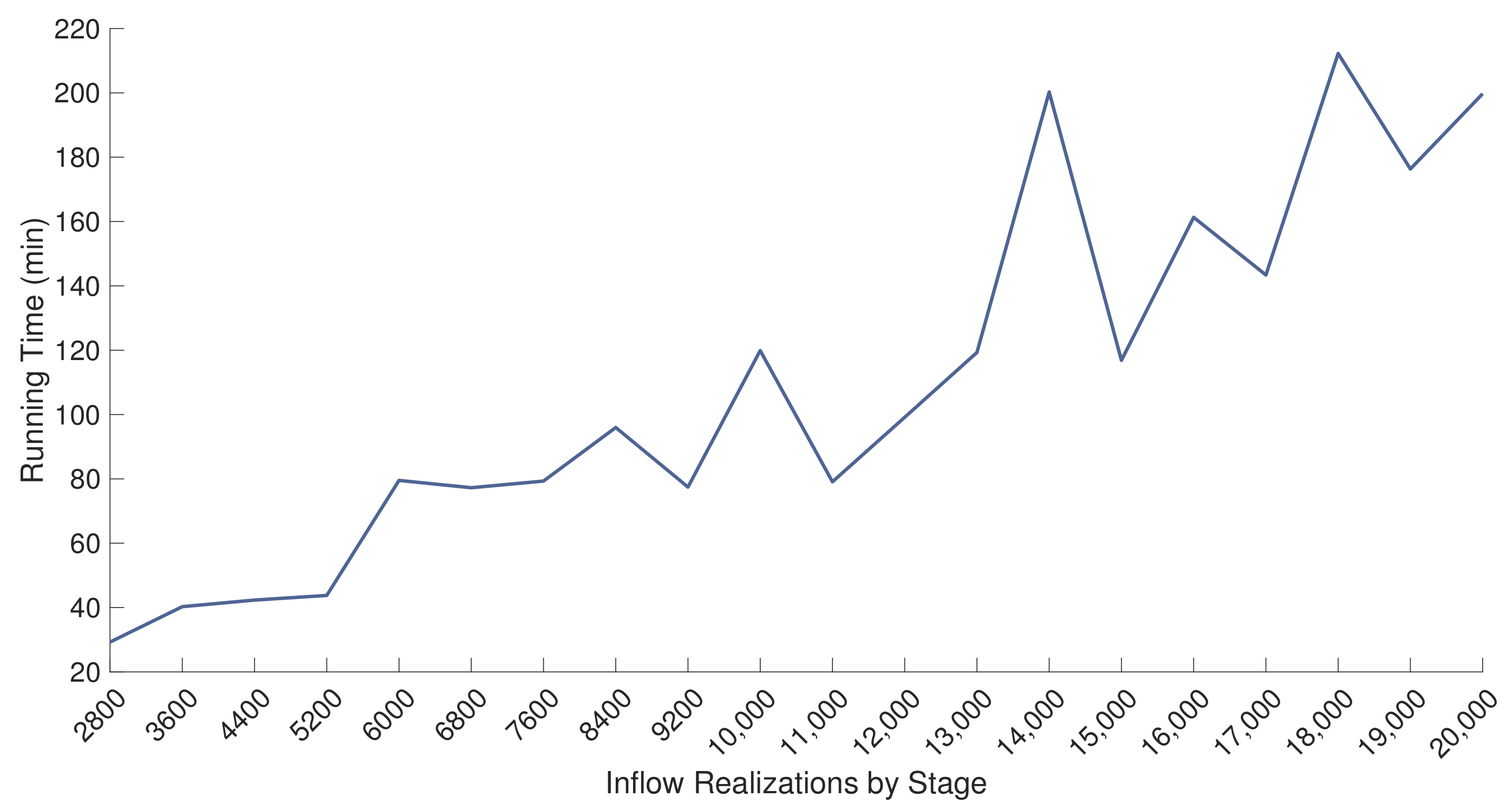
4.2.4. Computational Complexity

To assess the practical value of this research, we analyse two aspects of the SDDP: the running time needed to execute the algorithm and the runtime required to perform the solution quality evaluation. First, we specify that the SDDP algorithm is implemented in Fortran 90 and the DENSE_LP function in the IMSL numerical library is employed to solve the associated linear programming problems on a computer with the following characteristics: Intel Core $i7-6700HQ$ CPU @ $2.60$ GHz, $16.0$ GB RAM, $\times 64$ based processor. As reported by many authors, stochastic programming models are computationally expensive in terms of runtime. In this research, a large number of samples per stage have been considered, in turn resulting in scenario trees that are very large, as shown in Table 11. This fact raises the necessity to quantify the time needed to solve the associated problems. Figure 20 presents the computational time required to obtain the operating policies for the last 10 case studies.

As the size of the problem increases, it is reasonable to expect that the runtime required to solve it increases as well, and this behavior can be appreciated in Figure 20. Nevertheless, there are several cases where this does not occur because when the number of inflow realizations per stage increases, the computational effort needed to perform the backward simulations also increases. However, the number of iterations required to achieve convergence does not necessarily increase because the inflow scenarios (and the scenario trees) are different. Moreover, from the runtime point of view, it is less expensive to solve a problem with a wetter hydrological condition than one with a drier condition where it is necessary to resort to a greater extent to the thermal dispatch. Additionally, Figure 20 presents the runtime incurred on average; it can be noted that for the largest sample size studied, the average time needed is about 30 min, which is very acceptable. Nevertheless, it is worth mentioning that the problem investigated in this work is a small one, in the sense that 12 months are considered, while the planning horizon length of the Mexican MTHS problem is is actually up to 36 months. Moreover, it is assumed that the Infiernillo reservoir is isolated but it actually belongs to a cascaded system. Furthermore, given that within the simulations performed the one that demands more computational resources is the lower-bound estimation on the optimal solution of the original stochastic program, it is mandatory to quantify the total runtime required to solve the associated problems. This is displayed in Figure 21, which reveals that as the problem size increases, the runtime incurred to solve it also increases. Since the total runtime required to solve the large case studied is about 200 min, we consider that the runtime of the simulations is acceptable, despite the fact that the approach adopted to estimate the theoretical solution is computationally intensive. However, for large problems this approach can result in prohibitive runtime. For the estimation of the upper bound on the policy cost, the runtime is 1 min on average, even though each operating policy was simulated over 10,000 in inflow scenarios.

5. Conclusions

This work provides the best operating policies for the medium-term operation planning of a hydrothermal power system composed by the Infiernillo hydropower plant. The stochastic nature of inflows was included in the optimization problem using a scenario tree generated by Monte Carlo simulation and the probability distribution function that best fits each month of the historical record. The SDDP algorithm was implemented in Fortran 90, simulating one forward scenario per iteration and utilizing the stabilization of the first stage total operating cost as the convergence criterion. Additionally, we evaluated the policy quality by estimating the upper bound on the optimality gap and investigated 30 case studies by increasing the size of the scenario trees to identify the branch size with which it is possible to compute the best operating policies considering a trade-off between the solution quality and the computational effort involved. Then, to build the scenario trees, we utilized five randomly generated seeds so that the solution quality only depended on the branch size and not on the seeds employed, which led to the evaluation of a total of 150 operating policies. This paper shows that the best operating policy was obtained with a scenario tree generated with 17,000 inflow realizations by stage. Once the best operating policy was obtained, it was simulated over 10,000 inflow scenarios to estimate the expected value along the study horizon of the main variables involved in the MTHS problem. Moreover, the computational complexity was investigated to show that the runtime obtained in each stage of the simulation process was competitive from a practical point of view. Finally, we consider that the main contribution of this work was the determination of the system operating policy of an instance of the Mexican MTHS problem through the SDDP algorithm, aiming to represent an additional motivation to consider stochastic models while making decisions regarding the medium-term operation planning of the Mexican power system.

References

1. International Renewable Energy Agency (IRENA). Remap 2030 A Renewable Energy Roadmap; International Renewable Energy Agency: Masdar City, United Arab Emirates, 2014; Available online: https://www.irena.org/publications/2014/Jan/REmap-2030-Summary-of-findings-January-2014 (accessed on 1 January 2022).
2. United Nations Environment Programme and Centre, Frankfurt School-UNEP and Finance, Bloomberg New Energy. Global Trends in Renewable Energy Investment 2015; United Nations: New York, NY, USA, 2015. [Google Scholar]
3. International Renewable Energy Agency (IRENA). Renewable Energy Market Analysis: Latin America; International Renewable Energy Agency: Masdar City, United Arab Emirates, 2016; Available online: https://www.irena.org/publications/2016/Nov/Renewable-Energy-Market-Analysis-Latin-America (accessed on 1 March 2021).
4. United Nations Environment Programme and Frankfurt School-UNEP Centre and Bloomberg New Energy Finance. Global Trends in Renewable Energy Investment 2016; United Nations: New York, NY, USA, 2016. [Google Scholar]
5. Kelman, R.; Harrison, D. Integrating Renewables with Pumped Hydro Storage in Brazil: A Case Study; HAL: Lyon, France, 2019; pp. 1–23. [Google Scholar]
6. Electric Power Research Center (EPRI). Flexible Operation of Hydropower Plants; Electric Power Research Center: Palo Alto, CA, USA, 2017; pp. 1–76. [Google Scholar]
7. Siemonsmeier, M.; Baumanns, P.; van Bracht, N.; Schönefeld, M.; Schönbauer, A.; Moser, A.; Dahlhaug, O.; Heidenreich, S. Hydropower Providing Flexibility for a Renewable Energy System: Three European Energy Scenarios; The European Union: Brussels, Belgium, 2018; pp. 1–79. [Google Scholar]
8. Wolfgang, O.; Henden, A.L.; Belsnes, M.M.; Baumann, C.; Maaz, A.; Schäfer, A.; Moser, A.; Harasta, M.; Døble, T. Scheduling when Reservoirs are Batteries for Wind- and Solar-power. Energy Procedia 2016, 87, 173–180. [Google Scholar] [CrossRef]
9. International Energy Agency (IEA). Energy Policies Beyond IEA Countries: Mexico 2017; International Energy Agency: Paris, France, 2017. [Google Scholar]
10. Araripe Neto, T.A.; Cotia, C.B.; Pereira, M.V.F.; Kelman, J. Comparison of Stochastic and Deterministic Approaches in Hydrothermal Generation Scheduling. In Proceedings of the IFAC Symposium on Planning and Operation of Electric Energy Systems, Rio de Janeiro, Brazil, 22–25 July 1985. [Google Scholar]
11. Ceciliano, J.L.; Álvarez, J.; De-la-Torre, A.; Nieva, R.; Guillén, I.; Navarro, R.; Perales, F.; Torres, C.; Sánchez, A.; Yildirim, M.B. Power System Operator in Mexico Reveals Millions in Savings by Updating its Short-Term Thermal Unit Commitment Model. Interfaces 2016, 46, 493–502. [Google Scholar] [CrossRef]
12. Treistman, F.; Maceira, M.E.; Penna, D.D.; Machado, J.; Rotunno, O. Synthetic Scenario Generation of Monthly Streamflows Conditioned to the El Niño-Southern Oscillation: Application to Operation Planning of Hydrothermal Systems. Stoch. Environ. Res. Risk Assess. 2020, 34, 331–353. [Google Scholar] [CrossRef]
13. Gonçalves, R.E.C.; Finardi, E.C.; Da Silva, E.L.; Dos Santos, M.L.L. Comparing Stochastic Optimization Methods to Solve the Medium-Term Operation Planning Problem. Comput. Appl. Math. 2011, 30, 289–313. [Google Scholar] [CrossRef]
14. Larroyd, P.V.; De Matos, V.L.; Finardi, E.C. Assessment of Risk-Averse Policies for the Long-Term Hydrothermal Scheduling Problem. Energy Syst. 2017, 8, 103–125. [Google Scholar] [CrossRef]
15. Terry, L.A.; Pereira, M.V.F.; Araripe Neto, T.A.; Silva, L.F.C.A.; Sales, P.R.H. Coordinating the Energy Generation of the Brazilian National Hydrothermal Electrical Generating System. Interfaces 1986, 16, 16–38. [Google Scholar] [CrossRef]
16. Pereira, M.V.F.; Pinto, L.M.V.G. Stochastic Optimization of a Multireservoir Hydroelectric System: A Decomposition Approach. Water Resour. Res. 1985, 21, 779–792. [Google Scholar] [CrossRef]
17. Souza, R.C.; Marcato, A.L.M.; Dias, B.H.; Oliveira, F.L.C. Optimal Operation of Hydrothermal Systems with Hydrological Scenario Generation through Bootstrap and Periodic Autoregressive Models. Eur. J. Oper. Res. 2012, 222, 606–615. [Google Scholar] [CrossRef]
18. Oliveira, F.L.C.; Souza, R.C.; Marcato, A.L.M. A Time Series Model for Building Scenarios Trees Applied to Stochastic Optimisation. Int. J. Electr. Power Energy Syst. 2015, 67, 315–323. [Google Scholar] [CrossRef]
19. Calili, R.F.; Souza, R.C.; Galli, A.; Armstrong, M.; Marcato, A.L.M. Estimating the Cost Savings and Avoided CO2 Emissions in Brazil by Implementing Energy Efficient Policies. Energy Policy 2013, 67, 4–15. [Google Scholar] [CrossRef]
20. Brigatto, A.; Street, A.; Valladão, D.M. Assessing the Cost of Time-Inconsistent Operation Policies in Hydrothermal Power Systems. IEEE Trans. Power Syst. 2017, 6, 4541–4550. [Google Scholar] [CrossRef]
21. Rosemberg, A.; Street, A.; Dias, J.; Silva, T.; Valladao, D.; Dowson, O. HydroPowerModels.jl: A Julia/JuMP Package for Hydrothermal Economic Dispatch Optimization. Proc. JuliaCon Conf. 2020, 1, 35. [Google Scholar]
22. Andrieu, L.; Henrion, R.; Römisch, W. A Model for Dynamic Chance Constraints in Hydro Power Reservoir Management. Eur. J. Oper. Res. 2010, 207, 579–589. [Google Scholar] [CrossRef]
23. Van Ackooij, W.; Henrion, R.; Möller, A.; Zorgati, R. Joint Chance Constrained Programming for Hydro Reservoir Management. Optim. Eng. 2014, 15, 509–531. [Google Scholar] [CrossRef]
24. Philpott, A.; De Matos, V.L.; Finardi, E.C. On Solving Multistage Stochastic Programs with Coherent Risk Measures. Oper. Res. 2013, 61, 957–970. [Google Scholar] [CrossRef]
25. De Queiroz, A.R. A Sampling-Based Decomposition Algorithm with Application to Hydrothermal Scheduling: Cut Formation and Solution Quality. Ph.D. Thesis, The University of Texas at Austin, Austin, TX, USA, 2011. [Google Scholar]
26. De Matos, V.L.; Morton, D.P.; Finardi, E.C. Assessing Policy Quality in a Multistage Stochastic Program for Long-Term Hydrothermal Scheduling. Ann. Oper. Res. 2016, 253, 713–731. [Google Scholar] [CrossRef]
27. Finardi, E.C.; Decker, B.U.; De Matos, V.L. An Introductory Tutorial on Stochastic Programming Using a Long-Term Hydrothermal Scheduling Problem. J. Control. Autom. Electr. Syst. 2013, 3, 361–376. [Google Scholar] [CrossRef]
28. Pereira, M.V.F.; Pinto, L.M.V.G. Multi-Stage Stochastic Optimization Applied to Energy Planning. Math. Program. 1991, 52, 359–375. [Google Scholar] [CrossRef]
29. Pineiro, M.E. Stochastic Dual Dynamic Programming Applied to the Energetic Operation Planning of Hydrothermal Systems with Inflows Stochastic Process Representation by Periodic Auto-Regressive Models; Electrical Energy Research Center (Cepel): Rio De Janeiro, Brazil, 1993. (In Portuguese) [Google Scholar]
30. De Matos, V.L.; Finardi, E.C. A Computational Study of a Stochastic Optimization Model for Long Term Hydrothermal Scheduling. Int. J. Electr. Power Energy Syst. 2012, 43, 1443–1452. [Google Scholar] [CrossRef]
31. Kelman, J.; Kelman, R.; Pereira, M.V.F. Firm Energy of Hydroelectric Systems and Multiple uses of Water Resources. Braz. J. Water Resour. 2010, 9, 189–198. (In Portuguese) [Google Scholar]
32. Da Costa, J.P.; De Oliveira, G.C.; Legey, L.F.L. Reduced Scenario Tree Generation for Mid-term Hydrothermal Operation Planning. In Proceedings of the 2006 9th International Conference on Probabilistic Methods Applied to Power Systems, PMAPS, Stockholm, Sweden, 11–15 June 2006. [Google Scholar]
33. Sen, S.; Higle, J.L. An Introductory Tutorial on Stochastic Linear Programming Models. Interfaces 1999, 22, 33–61. [Google Scholar] [CrossRef]
34. Birge, J.R.; Louveaux, F. Introduction to Stochastic Programming; Springer: New York, NY, USA, 2011. [Google Scholar]
35. Infanger, G.; Morton, D.P. Cut Sharing for Multistage Stochastic Linear Programs with Interstage Dependency. Math. Program. Ser. A B 1996, 75, 241–256. [Google Scholar] [CrossRef]
36. Homem-De-Mello, T.; De Matos, V.L.; Finardi, E.C. Sampling Strategies and Stopping Criteria for Stochastic Dual Dynamic Programming: A Case Study in Long-Term Hydrothermal Scheduling. Energy Syst. 2011, 2, 1–31. [Google Scholar] [CrossRef]
37. Shapiro, A. Analysis of Stochastic Dual Dynamic Programming Method. Eur. J. Oper. Res. 2010, 209, 63–72. [Google Scholar] [CrossRef]
38. De Matos, V.L. A Model for the Annual Energetic Operation Planning Considering Advanced Stochastic Programming Techniques. Ph.D. Thesis, Federal University of Santa Catarina, Florianopolis, Brazil, 2012. (In Portuguese). [Google Scholar]
39. Da Silva, E.L.; Finardi, E.C. Parallel Processing Applied to the Planning of Hydrothermal Systems. IEEE Trans. Parallel Distrib. Syst. 2003, 14, 721–729. [Google Scholar] [CrossRef]
40. Shapiro, A.; Tekaya, W.; Da-Costa, J.P.; Soares, M.P. Report for Technical Cooperation between Georgia Institute of Technology and ONS; Georgia Institute of Technology and National System Operator: Atlanta, GA, USA, 2011. [Google Scholar]
41. Philpott, A.; Pritchard, G. EMI-DOASA; Electric Power Optimization Centre: Cambridge, MA, USA, 2013. [Google Scholar]
42. Fredo, G.L.M.; Finardi, E.C.; De Matos, V.L. Assessing Solution Quality and Computational Performance in the Long-Term Generation Scheduling Problem Considering Different Hydro Production Function Approaches. Renew. Energy 2018, 131, 45–54. [Google Scholar] [CrossRef]
43. Chiralaksanakul, A.; Morton, D.P. Assessing Policy Quality in Multi-Stage Stochastic Programming; Humboldt-Universität zu Berlin, Mathematisch-Naturwissenschaftliche Fakultät II, Institut für Mathematik: Berlin, Germany, 2004. [Google Scholar]
44. Shapiro, A.; Philpott, A. A Tutorial on Stochastic Programming. Tutorial 2007, 131, 45–54. [Google Scholar]
45. International Hydropower Association (IHA). 2018 Hydropower Status Report: Sector Trends and Insights; International Hydropower Association: London, UK, 2018; Available online: https://www.hydropower.org/publications/2018-hydropower-status-report (accessed on 1 June 2022).
46. Arganis, M.L.; Mendoza, R.; Domínguez, R.; Carrizosa, E. Operating Policies of El Infiernillo Dam for Hydropower Electricity Generation with Stochastic Dynamic Programming. Ribagua 2015, 2, 97–104. (In Spanish) [Google Scholar]
47. Ministry of Energy (SENER). Renewable Energies Outlook 2016–2030. Available online: https://www.gob.mx/sener/documentos/energy-sector-outlooks-2016-2030 (accessed on 1 February 2021).
48. Federal Electricity Commission (CFE)—Sub Direction of Non-Regulated Businesses. Meteorological Synopsis and Preliminar Forecasting, January 4th, 2021; Federal Electricity Commission: Mexico City, Mexico, 2021. (In Spanish) [Google Scholar]
49. Arganis, M.L.; Mendoza, R.; Domínguez, R. Operation of Three Hydroelectric Dams using Guide Curves and Stochastic Dynamic Programming. Water Technol. Sci. 2012, 3, 97–114. (In Spanish) [Google Scholar]
50. Feldman, R.M.; Valdez-Flores, C. Applied Probability and Stochastic Processes; Springer: Berlin/Heidelberg, Germany, 1996. [Google Scholar]
Figure 1. Decision process in hydrothermal systems.
Energies 16 06288 g001
Figure 2. Test system.
Energies 16 06288 g002
Figure 3. Two-stage scenario tree.
Energies 16 06288 g003
Figure 4. Three-stage scenario tree built under the interstage independent setting.
Energies 16 06288 g004
Figure 5. Historical record of monthly inflows.
Energies 16 06288 g005
Figure 6. Statistical measures of the real data.
Energies 16 06288 g006
Figure 7. Historical records’ box plots.
Energies 16 06288 g007
Figure 8. Skewness and kurtosis of the real data.
Energies 16 06288 g008
Figure 9. Evolution of the total operating cost, considering a branch size of 20,000 inflow realizations by stage.
Energies 16 06288 g009
Figure 10. Total operating costs evolution.
Energies 16 06288 g010
Figure 11. Evolution of the expected policies’ costs.
Energies 16 06288 g011
Figure 12. Sampling error evolution in the estimation of the upper bound on the expected policies’ costs.
Energies 16 06288 g012
Figure 13. Expected value evolution of total operating costs.
Energies 16 06288 g013
Figure 14. Sampling error evolution in the estimation of the lower bound on the optimal solution of the original stochastic program.
Energies 16 06288 g014
Figure 15. Upper-bound evolution of the optimality gap (USD).
Energies 16 06288 g015
Figure 16. Evolution of immediate and future operating costs.
Energies 16 06288 g016
Figure 17. Evolution of the energy generation of power plants.
Energies 16 06288 g017
Figure 18. Marginal cost of operation and water value.
Energies 16 06288 g018
Figure 19. Evolution of hydropower plant decision variables.
Energies 16 06288 g019
Figure 20. Computational time required to obtain the corresponding operating policies associated to the last 10 case studies.
Energies 16 06288 g020
Figure 21. Computational time required to estimate the lower bound on the optimal solution of the original stochastic program.
Energies 16 06288 g021