1. Introduction
The requirements for the static and dynamic properties of currently used drives are constantly increasing. The aim is to achieve short rise times, small overshoots, and vibration damping, also in the case of changing system parameters. With such requirements, all elements which can influence the drive property should be taken into account during the design procedure. In the drive, one of the most important factors that can reduce the performance is the characteristics of the mechanical part of the drive, in particular, the elasticity of the mechanical connection. Such drives are commonly called two-mass (or in general multi-mass) systems [
1,
2,
3,
4,
5,
6,
7,
8,
9,
10,
11,
12]. Classic examples are high-power, large inertia drives with elasticity resulting from the long connection between the driving motor and load machine. As an example, systems such as wind turbines, rolling mills, trains, and machines used in textile and paper industries can be mentioned [
1,
2,
3,
4,
5,
6,
7,
8,
9,
10,
11,
12]. If the mechanical characteristic is omitted in the process of designing the control structure, torsional vibrations may occur during the operation of the drive. They generate additional mechanical stresses in the shaft, decrease the whole system’s reliability, and shorten the life cycle of the system. Additionally, the torsional vibrations affect the accuracy of the position/speed control. The progress in power electronics and control techniques allows for the shortening of the time control of the driving torque in different motors. This, in fact, excited the torsional vibration in different types of drive systems. Nowadays, they are recognized in robotic arms, beams, and servo systems, as well as in the drives of vehicles, drones, and helicopters [
1,
2,
3,
4,
5,
6,
7,
8,
9,
10,
11,
12]. The control of torsional vibrations has been a very popular topic for decades, yet new, more effective control algorithms are sought after in industries.
In order to dampen torsional vibrations, different control strategies have been proposed. It has been shown in many papers that a classic cascade structure with a single PI controller is not a sufficient solution in this case [
13,
14]. This system can have large overshoots and long settling times. In order to increase the damping ability, the insertion in the control structure of one additional feedback from a selected variable is a standard solution. The use of two additional feedback allows us to locate the system’s closed-loop poles independently [
15]. The similar properties of the system ensure the state of the controller [
16]. The application of forced dynamic control additionally allows for the rejection of the effects of the load torque [
17,
18]. The use of a disturbance observer is also a very popular approach in such drives. There are many papers that describe the implementation of this technique [
19,
20]. In recent years, the model predictive control has become popular in many branches, including power electronics and electrical drives [
21,
22,
23,
24,
25,
26,
27]. There are also a number of works describing its application in vibration-damping problems. The main advantage of the MPC is better dynamics of the drive as well as the possibility of limiting the system state variables effectively. The mentioned disadvantage of the MPC is the computational complexity of the algorithm and stability issues.
The control problem becomes more complicated in the case of changeable parameters of the plant [
28,
29,
30]. In the case of a two-mass system, the moment of inertia of the load machine can vary in a wide range. To control such a plant, a robust or adaptive control is recommended. In the first group, approaches based on H∞ or µ-synthesis can be mentioned. However, the obtained solution is quite complicated [
31]. The sliding mode control is said to be a robust control algorithm [
32]. The system trajectory can be divided into initial reaching and then final sliding phases where the system is robust against disturbances. However, the drawback of this approach is a chattering phenomenon. Although there are available methods for chattering reduction, their implementation decreases the robustness of the control. The next methods are based on the application of fuzzy or neural controllers [
33]. The nonlinear control surface can increase the robustness of the plant, but the computational complexity of the algorithm increases at the same time. Additionally, tuning problems can be mentioned. The adaptive control can be separated into two groups. In the first one, the direct approaches are placed [
34,
35]. Based on the output of the plant (and reference signal) the parameters of the controller are calculated to minimize the tracking error. The indirect adaptive control can be treated as a second approach. The parameter of the controller is returned according to the estimated value of the changeable parameter(s) [
36]. Here, the significance of the estimation quality influences the properties of the system. The robustness of the MPC can be ensured in two different ways. The parameters of an internal model can be updated according to the estimated values. The second way is to use a special form of a cost function.
In order to implement an advanced (and robust) control algorithm, knowledge of the plant parameters and system states is necessary. Various algorithms can be used for this purpose. One of the simplest solutions is a disturbance observer; however, it estimates just the joint torque of the system, which is not enough for many structures. A commonly used solution is the full-order observer [
37]. It is a fairly simple algorithm; its coefficients can be determined using analytical formulas, and the required location of closed-loop poles of the system can be obtained. However, also in this case, the robustness to measuring noise and interference is limited. A definitely more complex algorithm, recommended especially for systems with high levels of noise, is the Kalman filter [
38]. Also, the moving horizon estimator can be used in this case [
39]. A different approach is represented by neural, fuzzy, or hybrid estimators, in which artificial intelligence methods are applied [
40,
41]. However, those systems are not popular in the industry yet. One of the drawbacks of the above-mentioned methods is the limited robustness to the initial states of the plant, especially in the case of a system with changeable parameters. Recently, the multilayer observer (MLO) has been proposed for the control problem of the two-mass system. It was shown in [
42,
43,
44] that the MLO can significantly reduce the estimation error of the system states and parameters in the case of unknown initial values and rapidly changing disturbances. This, in turn, improves the properties of the control structure.
The application of the robust MLO-based estimation system in electric two-mass systems is a new approach. To the best of the authors’ knowledge, there are no other works on this issue (excluding the author’s papers) in the literature. The previous paper [
43] focused on a detailed analysis of the MLO. The dynamic properties of the estimator are shown without focusing on the control structure. The main research problem in [
43] was a two-mass system with constant parameters but unknown initial conditions. The presented research shows that the observer is able to significantly increase the quality of the estimation in this case.
Contrary to [
43], the current work focuses on the problem of controlling a two-mass system with variable parameters. The robust control approach was chosen, in which the control structure has constant coefficients that ensure the repeatability of the speed courses despite changes in system parameters. Since the control structure requires information about state variables that are not measurable, it is important to provide an accurate and robust estimation system. This paper proposes the use of an MLO for this purpose. There are no works presenting this issue in the literature. Robustness is the result of both the regulator and the estimator. The increased accuracy of the estimator results from the selection of both its coefficients and the MLO structures. In order to show the effectiveness of the proposed control structure, the following approaches are presented in this paper. The first one relies on the application of control structures with direct feedback from all state variables. The parameters of the control structure are selected with the help of a global optimization technique with a specially selected cost function ensuring robust transients of the system states. This is an ideal case, which is a reference point for further research. The next system relies on the application of a control structure with a classical observer and an MLO. In both cases, the coefficients are also selected with the optimization algorithm. The obtained results are compared with a standard solution. The effectiveness of the system is examined under simulation and experimental study.
This paper is divided into six sections. After the introduction, the mathematical model of the drive and the considered control structure are presented. Then, the concepts of the MLO are described. The simulation results showing the design and properties of the robust control structure tested under simulation studies are placed in
Section 4. The laboratory setup and selected experimental tests are shown in
Section 5. In the end, the concluding remarks are placed.
2. Mathematical Model of Two-Mass System and the Control Structure
Many approaches evident in the literature can be used to model a two-mass system. Choosing one of them is a compromise between accuracy and computational complexity. Models based on finite elements allow for a very accurate analysis of phenomena in any element of the shaft. On the other hand, differential equation-based models are simple and suitable for the real implementation of control algorithms. Because the proposed control structure has to be implemented in real-time on the microprocessor system, the differential-equation-based model is implemented in this paper. It is described by the following state equations [
3]:
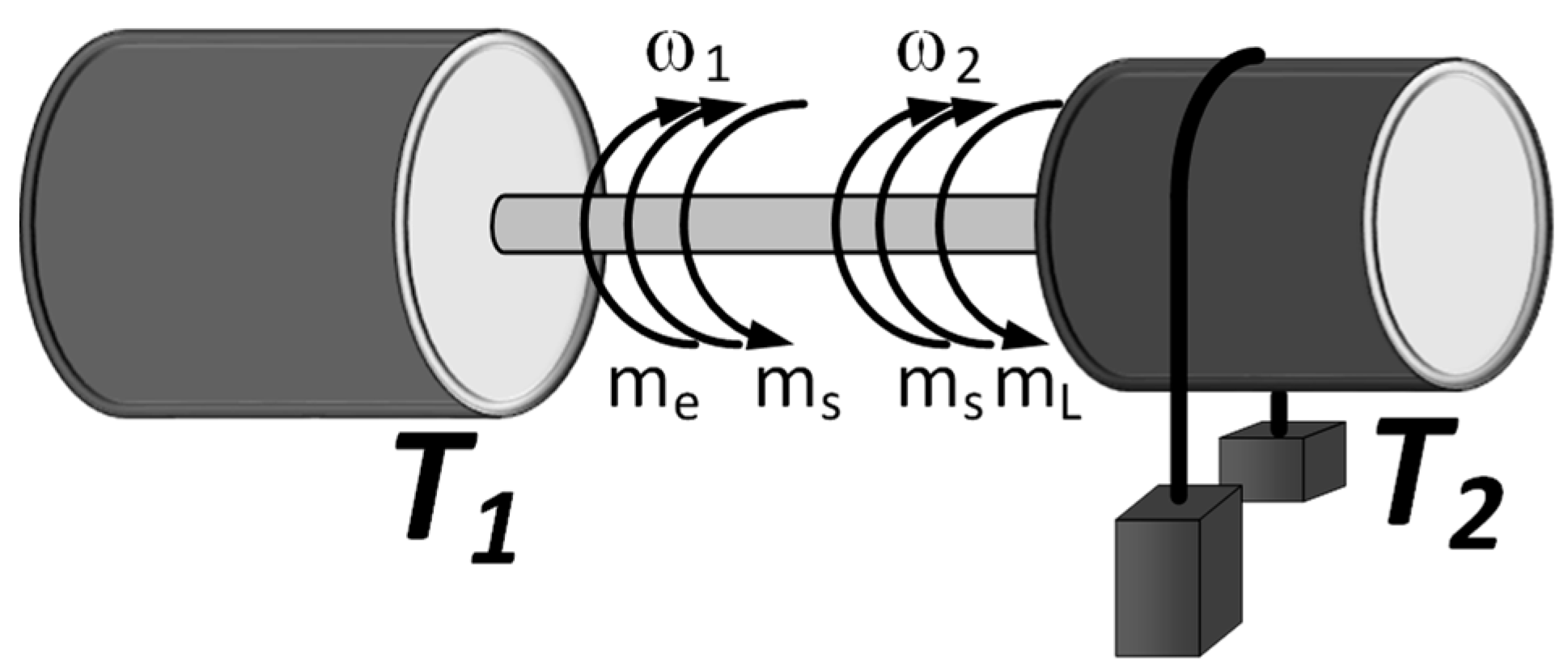
A schematic diagram of the two-mass system is presented in
Figure 1.
Three basic elements can be distinguished in the presented figure. These are, in turn, the moments of inertia associated with the driving motor and the working machine, and the long flexible shaft connecting those two elements. During work, the energy from the electrical supply system is used to develop an electromagnetic torque in the motor. The rotation of the motor affects the shaft, which develops the torsional torque, which in the end acts on the load side.
The classic speed control structure of an electric drive is a cascade control structure consisting of two loops, internal and external. The inner loop consists of the following elements: torque controller, power electronic converter, electromagnetic part of the motor, and current (and voltage) sensors. Depending on the type of motor, the torque regulator has a different structure. For example, for a DC motor, it is usually a PI controller. However, for an induction motor, the DFOC structure consists of several regulators. The task of the inner loop is to adjust the drive torque very quickly. In modern drives, this time is very short, even below 1 ms. For this reason, the dynamics of the inner loop are very often neglected when designing the outer loop. This means that the results obtained in this work can be applied to an electric drive with a different type of drive motor (DC, induction, or permanent magnet).
The external loop includes the following elements: drive torque control loop, mechanical part of the drive (single or multi-mass system), and position/speed sensor. The dynamics of the outer loop are mainly influenced by the mechanical parameters of the drive. Mechanical time constants are of primary importance here. Typically, their values range from several dozen to several hundred times higher than in the internal loop of the drive. The PI controller is usually applied in this loop.
Controlling a multi-mass system is a difficult issue. The basic task of the control structure is to effectively suppress torsional vibrations. This is due to their negative impact on the controlled object. Undamped vibrations can lead to a deterioration of the speed/position control parameters and, consequently, to variations in the quality of the manufactured product or to an increase in energy consumption. Torsional vibrations negatively affect the reliability of the system and, in special cases, can lead to damage. Another task of the control system is to ensure high dynamics of regulation of individual variables, usually the speed/position of the working machine.
The basic speed control system is a system with a PI controller without additional feedback. The controller settings are selected according to the methodology presented in [
15]:
A closed control system with a PI controller is a fourth-order system. Since there are only two parameters in the control structure, it is not possible to freely distribute the poles of a closed system. This limits the properties of the control structure.
In order to show the properties of the system with the PI controller, simulation tests were performed. The PI regulator settings were determined for the nominal parameters of the object. Simulation tests were carried out. Then, the time constant of the working machine was increased five times without changing the controller settings. Tests were carried out again. The determined waveforms are presented in
Figure 2.
As a result of the analysis of the waveforms presented, in the case of nominal parameters of the object, the system velocities have a slight overshoot. However, it should be emphasized that the speed increase time is quite slow. Changing the parameters of the object degrades the properties of the control structure. In the waveforms of the state variables, large overshoots and slowly damped oscillations are visible. This means that the classical control structure is not effective, especially in the case of an object with variable parameters. There are a lot of control structures that can be applied to dampen torsional vibrations effectively. As mentioned in the introduction, it can be structured based on the PI controller supported by different feedback, state controller, MPC, or others. Taking into account the properties: the possible ability to design the shape of the speeds of the system and implementation issues, the control structure with the PI controller with additional feedback from the shaft torque, and the difference between speeds are selected in this work. Since the closed control structure is fourth order, it allows the poles of the control system to be arranged independently. Thus, it is theoretically possible to both effectively suppress torsional vibrations and achieve the assumed rise time. However, it should be remembered that the assumption of very high control dynamics will require generating a large drive torque, which in practical systems may be impossible. Firstly, the control structure is described, and then the procedure of the robust closed-loop pole locations is presented.
The transfer function of the PI controller has the following form (3).
The coefficients of the control system are determined using the pole placement methodology described in detail in [
15]. The results are the analytical Formulas (4)–(7) that allow for the pole locations in the closed-loop system.
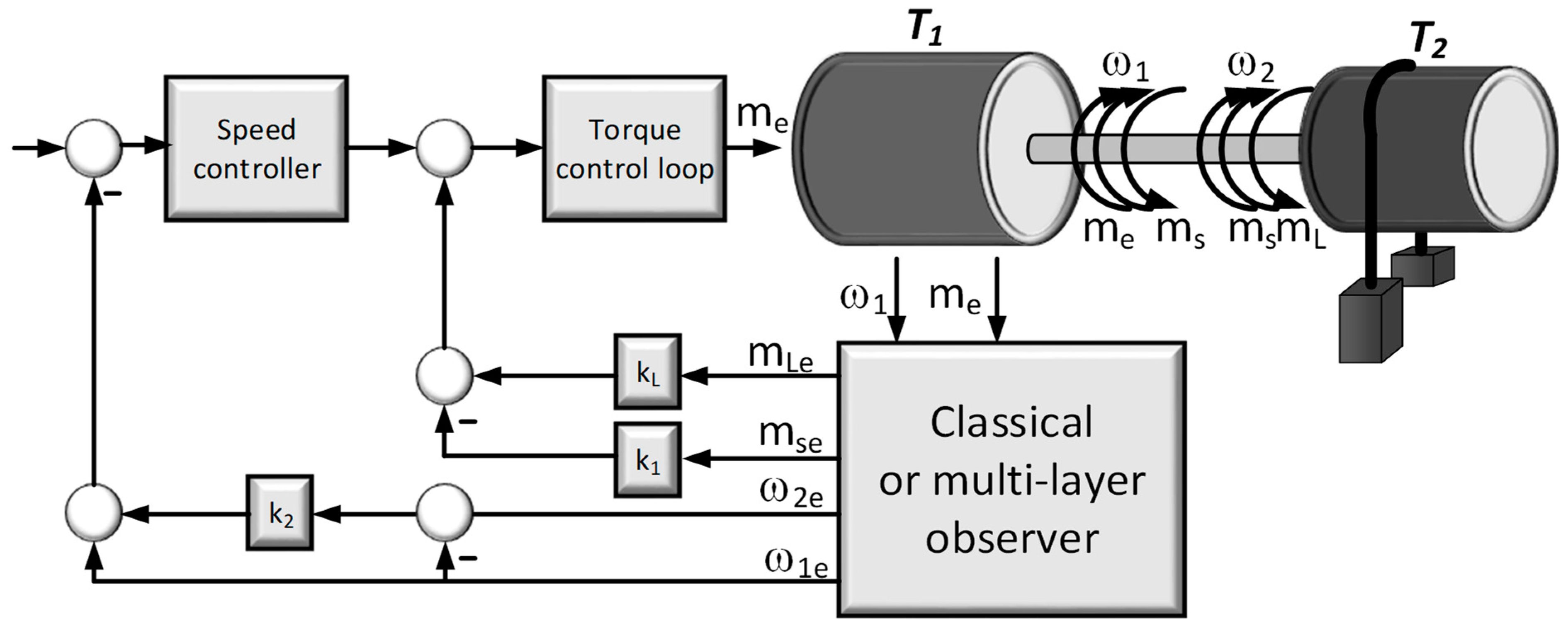
In order to implement the analyzed control structure, information on all state variables of the system is required. Since, in standard drive systems, only the motor speed and electromagnetic torque signals are available, it is necessary to use an estimator that determines the remaining state variables. In the present work, this role is performed by a multilayer observer. A diagram of the considered control structure working with the estimator is shown in
Figure 3.
The presented system has a cascade structure. In the inner loop, the electromagnetic torque is controlled. In the case of a DC motor, it can be realized with an armature current regulator, as well as for an induction motor, e.g., the DFOC system. Since the dynamics of the electromagnetic torque is significantly larger than the dynamics associated with the mechanical part, it is omitted in the process of selecting the settings of the control system. In the block diagram, an additional coefficient kL is visible. It is implemented to improve the reaction of the system to the applied load torque.
The presented Equations (4)–(7) allow us to obtain the desired transient of the system states in the case of constant parameters. However, in many drive systems, the parameters can vary within wide limits. This applies especially to the parameters of the working machine. For example, a robot arm can be mentioned here. In many cases, its distance from the axis of rotation changes, and thus the moment of inertia of the working machine changes. Another example is a wire winder or machines in the paper industry. The moment of inertia of the working machine changes with the amount of wound material. Another example is servo drives in machines that process solids of various shapes. The mechanical parameters of the long shaft change much less frequently. Their change indicates the degradation of the mechanical connection and indicates the possibility of damage to the drive.
The disadvantage of the presented analytical method is the dependence of individual expressions on constant (rated) parameters of the drive system. Since the time constant
T2 varies over a wide range, it is necessary to find another solution. One approach is to use the global optimization method. In this case, an important element is to define the objective function and then to select the coefficient values to achieve its minimum. In the current work, the following form of the objective function was adopted:
where
ωref—reference speed,
ω1U1/U2/U3 and
ω2U1/U2i/U3—speeds of the motor and load machine in cases:
U1 where
T2 =
T20 = 0.203 s,
U2 where
T2 = 3
T20 = 0.609 s, and
U3 where
T2 = 5
T20 = 1.015 s.
The application of the tuning procedure results in robust responses from the drive. Despite the changes in the system parameters, the speed transients of the working machine are similar.
3. Classical and Multilayer Observer
To implement the considered control structure, information about the state variables of the system is necessary. There are several methods to estimate state variables in the literature. They have different properties. Choosing one of them is a compromise between the numerical complexity of the estimator and its estimation quality, especially in the case of a noisy system. In this paper, the full-sized asymptotic observer is chosen. It is characterized by a relatively simple structure and an uncomplicated method of selecting correction factors. For this reason, it is used in many industrial applications. An increase in the quality of state variable estimation was obtained by using a multilayer observer. Below is a description of the classical full-sized asymptotic observer as well as the multilayer observer.
The classical full-size asymptotic observers are described in general by Equation (9):
The original state vector of the plant is extended by the load torque:
Information about the moment of the load allows the use of additional feedback in the considered control structure. It improves the properties of the system in case of changes in the load torque. The electromagnetic torque and the motor speed are the input and output of the system, respectively.
The state, control, and output matrices of the observer are defined as follows (12):
The matrix
K, which contains correction coefficients, is described, in turn, as (13):
The correction coefficients are determined using the following Equations (14)–(17):
where
p is the resonant frequency of the observer closed-loop poles and
a is the damping coefficient.
The presented equations allow for the arbitrary location of the poles of a closed system in the complex plane. Consequently, the dynamics of estimation error elimination can be shaped by the system designer. However, it should be remembered that very large gains cause additional oscillations in transients in the estimated variables. This is due to the presence of noise in the real system. For this reason, observer gains should be limited.
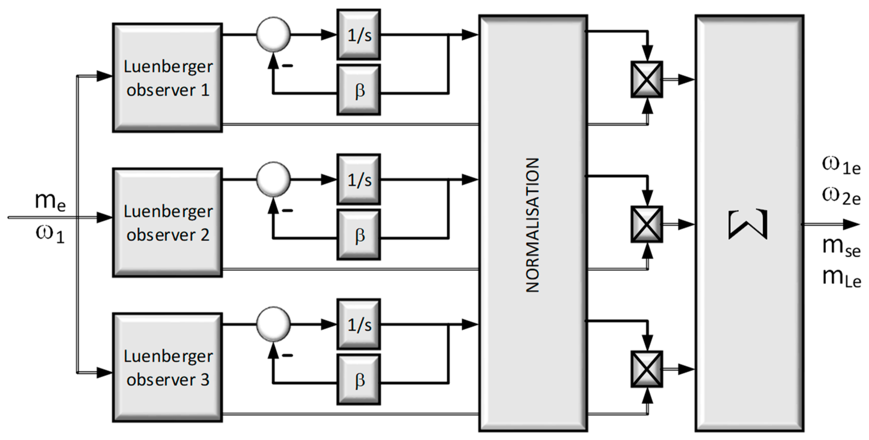
The full-sized asymptotic observer has limited resistance to measurements and parametric noises. Additional errors cause unknown initial states in the system. To improve the quality of the estimation, a multilayer observer was used. The block diagram of the multilayer observer is shown in
Figure 4. In the first layer, some estimators (usually two or three) work in parallel. In this work, there are three full-sized asymptotic observers with different initial conditions. It should be noted that there is a possibility of changing the conditions in the observers not only at the beginning but also during the operation of the system (in the presented system, this occurred after detecting changes in the load moment). In the second layer, based on the motor speed estimation error (difference between the measured speed and the value determined by a specific estimator), the weighting factors are calculated for each estimator (18). These coefficients are then normalized (19) so that the sum of the normalized weighting coefficients of all observers equals one (20), which makes the analysis of the properties of the system easier. Based on weighting factors and output signals from individual estimators of the first layer, the output signal of the multilayer observer (21) is determined.
where
γ—learning coefficient,
ω1—measured motor speed of,
—motor speed determined by the
i-th estimator from first layer,
αi,
αi—weighting factor of the
i-th estimator before and after normalization,
xi—output signal of the
i-th estimator, and
x—output signal of the multilayer estimator.
According to the presented relationships, the smaller the estimation error of a given observer, the greater its weighting factor after normalization, and thus the greater its contribution to the output signal of the multilayer system. The coefficient
ai (18) can be modified by applying the forgetting factor
β, to limit the increase in this coefficient in a finite time (22).
where
β—forgetting factor.
The classical estimator calculates state variables based only on the current measurement sample. For this reason, it has a finite resistance to changes in the parameters and initial states of the object. In a multilayer observer, we have a rear-facing window. The influence of a given observer on the final result is a consequence of not only the current sample but also several (several dozen) past samples.
The stability of the observer is one of the basic elements that should be investigated. The MLO consists of two layers. In the first, there are a number of individual systems. The stability of a single observer can be checked by spreading its poles. In the case of parameter selection using Equations (14)–(17), this is ensured analytically by placing the poles on the left side of the plane. In the case of the selection using the global optimization algorithm, the arrangement of the poles of the system should be checked. Since all observers in the first layer have identical settings (they differ only in initial states), the stability of one of them means the stability of all. In the second layer, there is an aggregation mechanism. It combines signals from individual observers into one signal. It does not affect the stability of the system. If the observers in the first layer are stable, then the whole system will be stable as well.
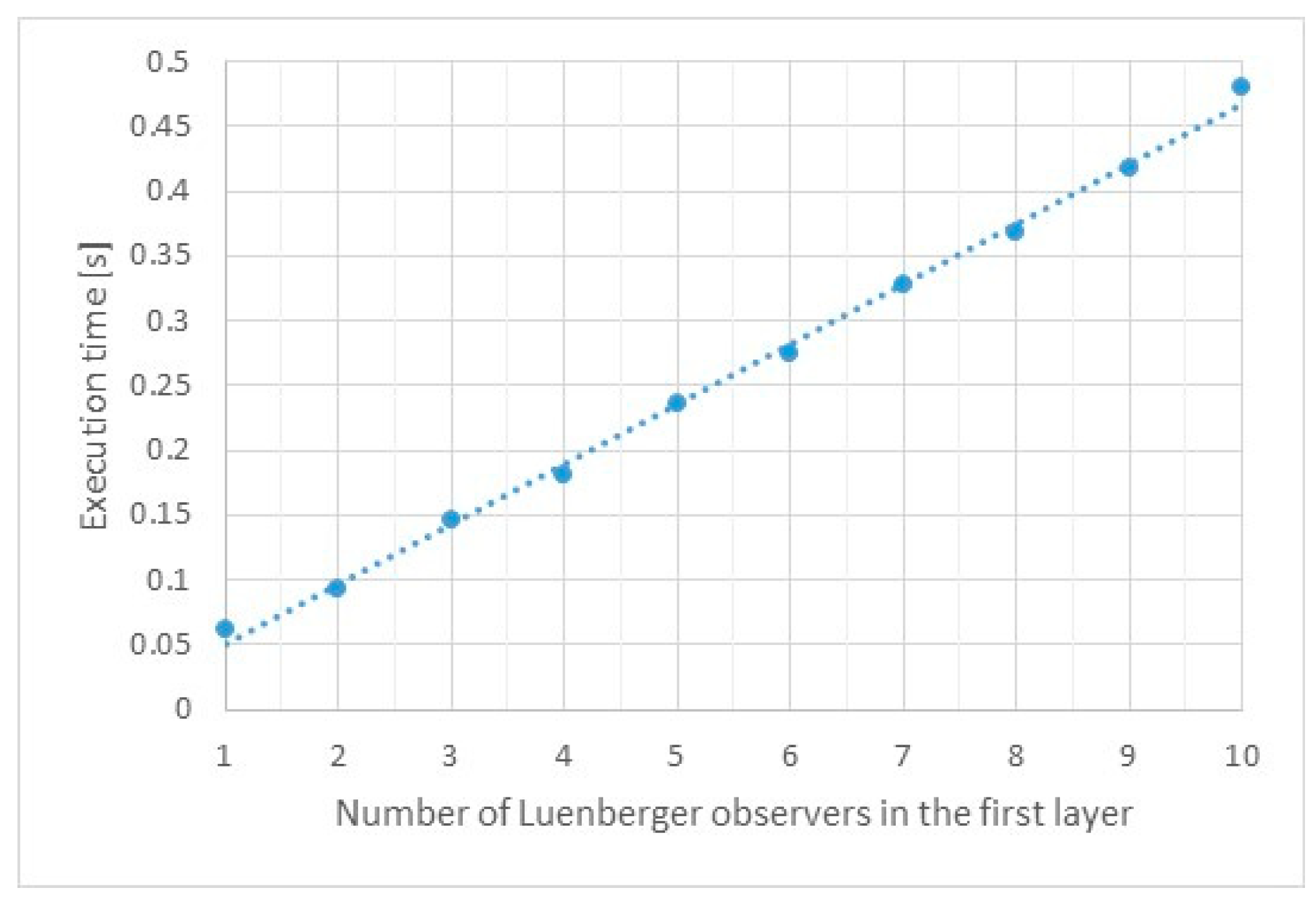
Another issue of practical importance is the computational complexity of the MLO system. It depends greatly on the type of single estimator used. It will be different when using the classical full-sized asymptotic observer than in the case of the Kalman filter. In this paper, complexity was determined in two ways. In the first one, the number of basic mathematical operations for the MLO with a different number of layers was counted. For the second method, it was decided to measure the execution time of a practical MLO with a different number of individual systems. To eliminate the effect of randomness, the calculations were performed 100,000 times.
Table 1 shows the values obtained.
MLO execution time with a different number of individual observers plotted in
Figure 5.
As can be seen from the data contained in
Table 1 and the graph above, the computational complexity of the MLO depends proportionally on the number of individual observers used in the first layer. On the one hand, increasing their number improves the quality of estimation of state variables; on the other hand, it is necessary to increase the computing power of the processor.
4. Simulation Results
The aim of the research is to design a control system that cooperates with the selected estimator and is robust to changes in the mechanical time constant of the working machine. In the control structure, there are a number of design coefficients related to the structure of the controller and the estimator. Since the analytical Formulas (4)–(7) work for constant parameters of the object, a different approach is chosen. In this paper, three systems are considered. The first one, theoretical, assumes the existence of information about all variables of the object’s state. In this case, the parameters of the structure are selected using an optimization algorithm in order to make it robust to the change in the time constant of the working machine. The second system consists of a control structure and a classical full-size asymptotic observer. All system coefficients (control structure and observer) are selected using an optimization algorithm. The third considered system is a control structure working with a multi-observer. In this case, the parameters of the structure and the multi-observer are also selected using an optimization algorithm. The use of the described procedure makes it possible to obtain optimal properties in each case.
In this paper, the pattern search algorithm is applied to find optimal values of the control coefficients. The initial settings are adopted according to the expressions ω0 = 40 s−1 and damping factor ξ = 0.7 and for the observers p = 80 s−1 and a = 0.7. In the optimization process, the objective function of form (8) is used. The disturbances evident in the plant are taken into account. A total of 100 iterations of the pattern-search algorithm is assumed.
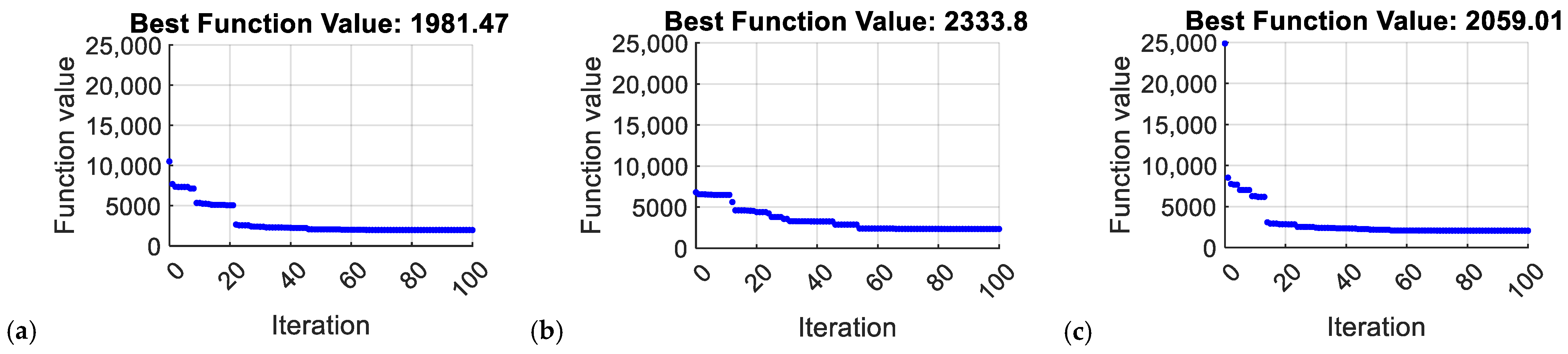
The optimization procedure was carried out several times. Similar results were obtained each time. The course of changes in the objective function, in the case of the best result for a particular system, is presented in
Figure 6. It shows the transients of the cost function during the optimization process for a system with direct feedback from the model as well as a classical and multilayer full-sized asymptotic observer. In the multilayer observer, the following initial conditions are adopted (according to the assumed state vector (9)): in system 1 [0,0,2,2], in system 2 [0,0,0,0], in system 3 [0,0,−2,−2], and in the model of a two-mass system [0,0,0,0].
Analyzing the graphs presented in
Figure 6, it can be seen that the theoretical system with direct feedback from state variables has the lowest target value. This is obvious because it has no estimator. The control structure working with a multi-observer has the value of the objective function higher by about 4%. In the case of a system cooperating with a classical observer, this value is higher by about 18%. This means that the system working with a multi-observer can provide much better properties than the system working with a classical observer.
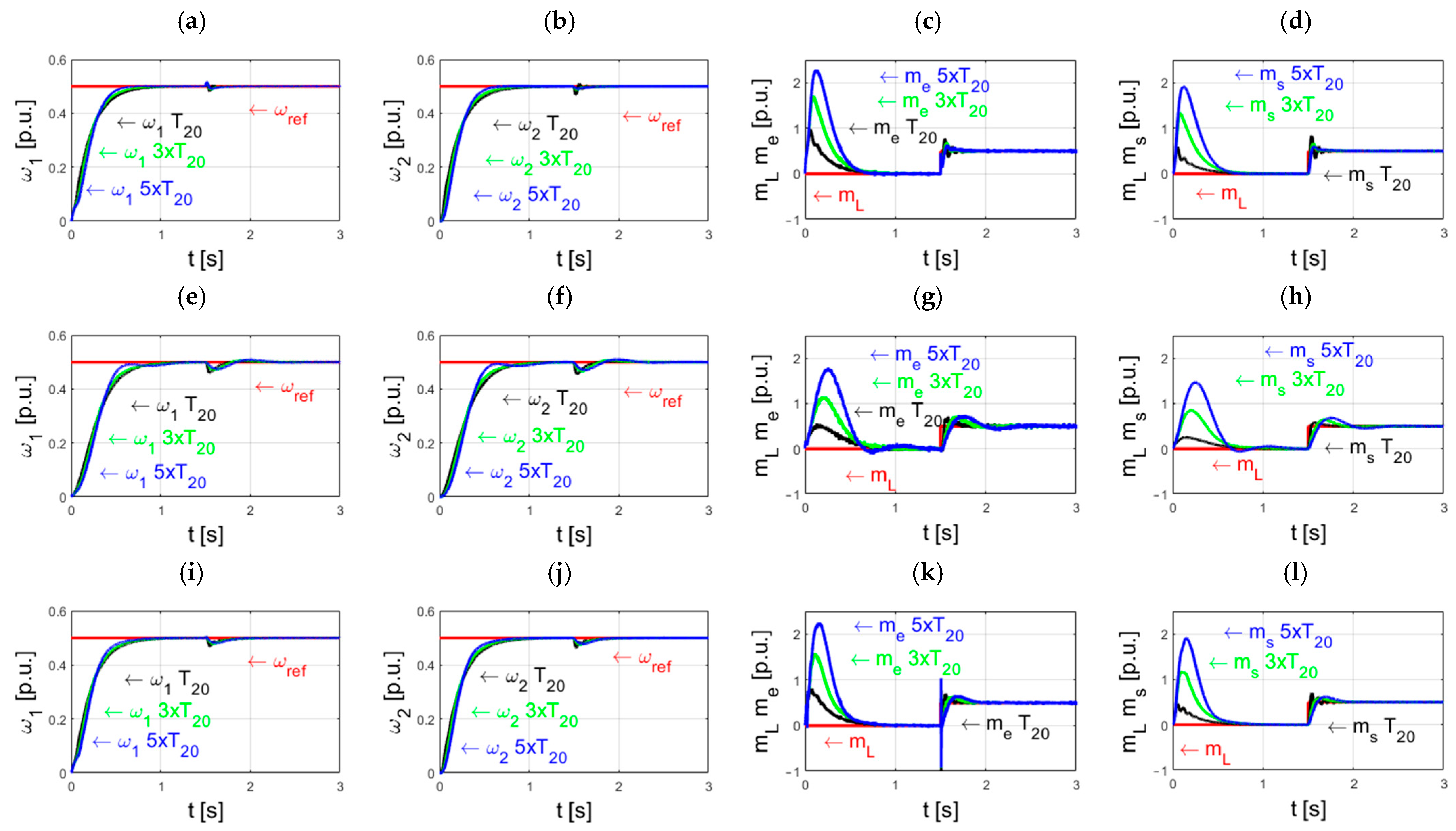
Then, simulation tests of three analyzed systems were carried out. Their goal was to check how individual systems regulate state variables in the case of rated and changed object parameters. In the simulation conditions, the start of the system was assumed from zero to the reference speed and the subsequent application of the load torque. The reference speed value is chosen to be half of the nominal value, in order to avoid the limitation of the driving torque. Selected waveforms of the system variables are shown in
Figure 7.
The first system, with direct feedback from all state variables, is analyzed. The speeds and torques curves of the system are shown in
Figure 7a–d, respectively. Each drawing contains collective waveforms recorded for three values of the mechanical time constant: nominal, three times, and five times increased. These waveforms serve as a comparison for successively analyzed cases. Then, systems with classical and multilayer Luenberger observer were investigated. The waveforms of individual state variables are shown in
Figure 7e–l, respectively, for the analyzed cases. As before, the figures show cumulative waveforms for three values of a variable parameter.
Based on the waveforms shown in
Figure 7, the following conclusions can be drawn. All systems work properly. The speed courses of the working machine are similar in all systems for different values of the time constant of the working machine. This proves the correctness of the selection of coefficients for the control structure. However, a closer analysis of the individual variables for different systems reveals some differences. They are most visible in the waveforms of the system’s moments. For example, for the largest value of
T2, the system with direct coupling forces the maximum value of the torsional moment to be equal to two. A similar value is reached in the structure working with a multi-observer. For a system that works with a classical observer, this value is close to 1.5. It is obvious that these differences must also be present for other variables. For example, speed courses in the system with a classical observer have the most oscillatory character. It should be emphasized that the robust controller with a multi-observer is characterized by a smaller discrepancy in the speed waveforms for different values of the time constant of the load machine (
T2). Based on the waveforms, it can be concluded that the behavior of the system cooperating with the multi-observer is more similar to the system with direct feedback.
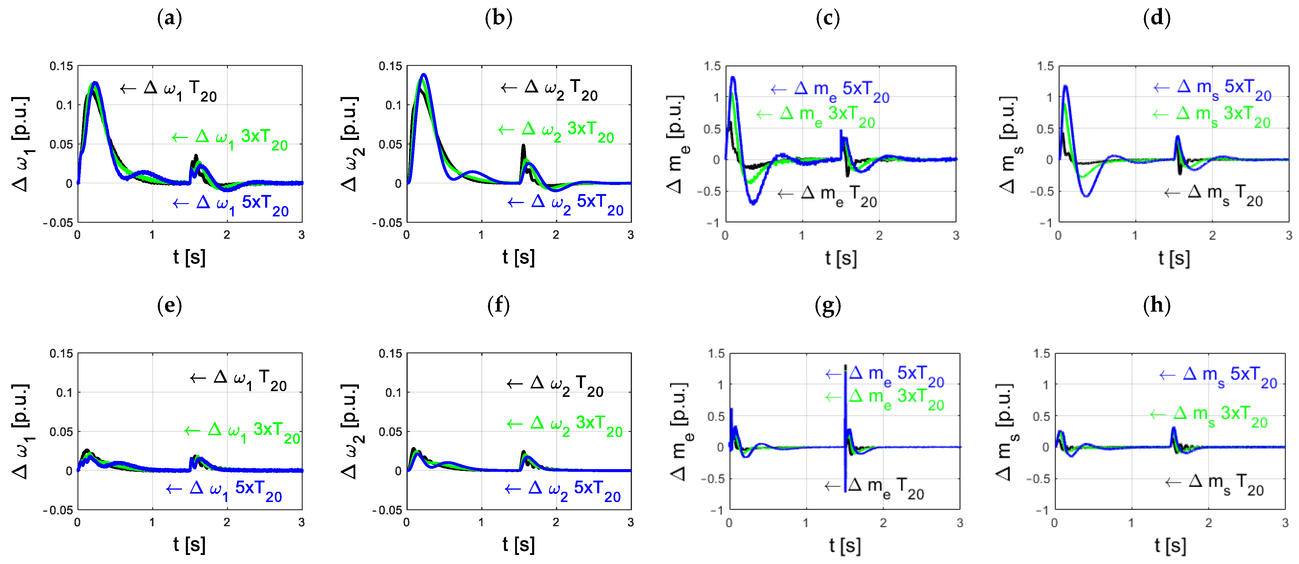
In order to show the differences more precisely,
Figure 8 shows the curves of the differences between the individual state variables of the system with direct coupling and two subsequent systems: working with a classical and a multi-observer.
The following conclusions can be drawn based on the analysis of error transients shown in
Figure 8. For the system operating with a classical observer, the speed errors reach the value of 0.14 (
Figure 8a,b); they are slightly larger for the load speed and rather independent of the value of the mechanical time constant of the working machine. For torque waveforms, these values are greater than 1.25 (
Figure 8c,d). In this case, they depend significantly on the
T2 parameter, for its greater value, larger errors arise. In the case of a system working with a multi-observer (
Figure 8e–h), these errors are several times smaller. The impact of
T2 changes on the error waveforms is similar to in the case described above. For speed errors, it is small (
Figure 8e,f) and for moments, it is large (
Figure 8g,h).
Subsequently, the error values are determined using the following formula:
where
vd—values of samples of variables from a system with direct feedback,
vc|m—values of samples of variables from a system with classical (
c) and multilayer observer (
m), and
N—number of samples.
The results in
Table 2 confirm the conclusions formulated above based on the waveforms in
Figure 8. The system that works with a classical observer has the largest estimation errors. For speeds, they are 4-times higher than for the system cooperating with a multi-observer. Additionally, increasing
T2 slightly increases the errors in the classical system. In the case of a multi-observer, this value is basically constant and does not depend on
T2. For the torque, the error values for the classical system are 3–4-times higher than that for the multi-observer. In this case, they depend on the value of
T2; its increase causes an increase in errors for the two systems.
5. Experimental Results
In the next stage of research, the operation of the developed systems is tested under laboratory conditions. During the tests, a set of two 500 W DC motors connected with a long (600 mm) flexible shaft is used. The driving motor is powered by an H-bridge. Incremental encoders with a resolution of 36,000 pulses are connected to both motors, while the control structure uses only the signal from the encoder on the side of the driving motor; the second one is used only to evaluate the estimation system. During the tests, the operation of the system is checked in the case of changes in the mechanical time constant of the load machine. These changes are made by attaching additional steel discs on the side of the load machine. The initial value of
T2 (resulting from the parameters of the working machine itself) is 0.203 s. For systems with additional discs with a thickness of 4, 8 and 16 mm, the
T2s are 1.015 s, 0.406 s, and 0.609 s, respectively. The picture of the laboratory setup is presented in
Figure 9.
Experimental studies are carried out as follows. Two systems are tested, one cooperating with a classical observer and the other with a multi-observer. The value of the reference speed is assumed to be at the level of 0.5, similar to that in simulation studies. Tests are carried out for the nominal value of the mechanical time constant
T2 = 203 ms and its 2-, 3- and 5-times higher value. The transients of the tested system are shown in
Figure 10.
Figure 10a,b,e,f shows the waveforms of the velocities and torques recorded for the two tested systems in the case of the smallest tested constant value
T2 = 203 ms. The following conclusions can be drawn from their analysis. The drive torque is forced more dynamically in the MLO structure (
Figure 10f) than in the classical observer structure (
Figure 10e). In the first case, its value reaches 0.9 of the rated torque and in the second, about 0.5. This results in different dynamics for the forcing speed (and torque) in the system. In the case of the MLO system, this speed is forced much faster than in the second case. It is also necessary to pay attention to the reaction of the system to a change in the load moment. In the case of the structure with MLO, dynamic torque forcing is visible, which results in smaller disturbances in speeds. Then, the case of changing the load torque to the value
T2 = 406 ms was tested. The courses of moments and speeds of the system are shown in
Figure 10c,d,g,h. In the case that the system cooperates with the MLO, a large difference in forcing the drive torque is still visible, both during changes in the set speed and changes in the load torque (
Figure 10h). This results in a more dynamic reaction in the speed of the system to the change in both signals. In the case of a system cooperating with a classical observer, this dynamic is definitely smaller. The maximum value of the driving torque in this case is about one, whereas for the MLO system, it is 1.4. Then, the system with the time constant
T2 increased to 909 ms was tested. The recorded waveforms are shown in
Figure 10i,j,m,n. As before, the dynamics of forcing all variables is faster in the system cooperating with the MLO than in the system with a classical observer. In addition, attention should be paid to the noise level in the system with a classical observer. It becomes more and more visible in this case. The last tested case was a system in which the value of the time constant
T2 was increased five times to 1.015 s. The speed courses of the drive motor and the working machine, as well as the electromagnetic and torsional torques, are shown in
Figure 10k,o for the system working with a classical observer and
Figure 10l,p for the system working with the MLO. A very high level of drive torque oscillation can be noticed in the system with a classical observer (
Figure 10o). These oscillations are transferred to the speed of the drive motor (
Figure 10k) in the initial period of start-up. The change in the load torque causes visible oscillations in this system. The system with the MLO works much better. There are no visible oscillations in the waveforms of the moments. In addition, the change in the load torque interferes with the operation of this system to a much lesser extent. The resulting velocity deformations are much smaller. The speed returns to the reference value much faster with this system.
Based on the presented results, it can be concluded that the speed stabilization is much better in the system cooperating with the multilayer observer. This system reacts faster to changes in the set speed and load torque. It should also be noted that the level of oscillation in the electromagnetic torque transients is greater in the case of using a classical observer. Despite these significant changes in the values of the estimated load torque, the system cooperating with the multilayer observer also works better in this case than the system with a classic observer, estimating the correct value of the load torque much faster and stabilizing the speed at the set value.


 ,
, 


