Adaptive Clustering Long Short-Term Memory Network for Short-Term Power Load Forecasting

Abstract

Short-term load forecasting (STLF) plays an important role in facilitating efficient and reliable operations of power systems and optimizing energy planning in the electricity market. To improve the accuracy of power load prediction, an adaptive clustering long short-term memory network is proposed to effectively combine the clustering process and prediction process. More specifically, the clustering process adopts the maximum deviation similarity criterion clustering algorithm (MDSC) as the clustering framework. A bee-foraging learning particle swarm optimization is further applied to realize the adaptive optimization of its hyperparameters. The prediction process consists of three parts: (i) a 9-dimensional load feature vector is proposed as the classification feature of SVM to obtain the load similarity cluster of the predicted days; (ii) the same kind of data are used as the training data of long short-term memory network; (iii) the trained network is used to predict the power load curve of the predicted day. Finally, experimental results are presented to show that the proposed scheme achieves an advantage in the prediction accuracy, where the mean absolute percentage error between predicted value and real value is only 8.05% for the first day.

1. Introduction

With the development of society, electricity plays a crucial role in industrial, commercial, and residential settings. It is essential to accurately predict variations in electricity load to ensure the stable operation of the power system [1]. Short-term load forecasting (STLF) is a vital aspect of energy forecasting that involves predicting instantaneous electricity load values at hourly intervals for the next day or several days [2,3,4]. STLF is critical for power system scheduling, energy optimization, and efficient operation of electricity markets [5]. However, STLF presents challenges due to its uncertainty and non-linear characteristics influenced by factors like weather conditions, holidays, seasons, and industrial production. This problem involves high randomness and difficulties in establishing mathematical models as well as selecting appropriate features [6]. Various algorithms and approaches have been proposed by scholars worldwide to improve the accuracy of load forecasting. These include time series forecasting (TSF) [7,8] and support vector machine (SVM) [9]. With the advancement of artificial intelligence, predictive methods based on deep learning have gained popularity due to their ability to approximate high-dimensional functions, uncover hidden information in data, and extract abstract features [10]. Deep learning is more robust compared to traditional TSF and SVM. Specifically, long short-term memory networks (LSTM) [10], a type of recurrent neural network, are preferred for addressing the vanishing gradient problem and improving performance in handling time series data. For short-term residential load forecasting, Ref. [11] introduced an LSTM-based framework that outperforms conventional backpropagation neural networks in experiments. In Ref. [12], a hybrid method combining variational mode decomposition with LSTM is studied for processing STLF. Additionally, Ref. [13] proposes a hybrid approach using multivariable linear regression and LSTM for short-term load forecasting. In order to improve prediction accuracy, researchers have utilized clustering analysis on the original load data. This involves dividing the data into clusters before making predictions [14]. Common clustering algorithms used for electricity load data include K-Means [15] and density-based spatial clustering of applications with noise (DBSCAN) [16]. For example, in Ref. [17], K-Means was used to classify users based on their electricity consumption patterns, and backpropagation (BP) neural networks were applied for short-term load forecasting. Ref. [18] combined deep learning with K-Means to extract similarities in residential load for accurate individual-level prediction. Additionally, a short-term support vector machine load forecasting method based on K-Means was proposed in Ref. [19], whereas a combination of K-Means and fuzzy processing techniques was used for short-term load prediction in Ref. [20]. Furthermore, ultra-short-term load forecasting involved employing K-Means to divide historical data into clusters and utilizing long and short-term time-series networks (LSTNet) as described in Ref. [21]. DBSCAN was also applied for cluster analysis followed by multiple neural networks for load forecasting according to another study’s approach [22]. Compared to previous methods such as K-Means and DBSCAN, our previous work introduced a maximum deviation similarity criterion (MDSC) clustering algorithm specifically designed for STLF. This algorithm demonstrated superior performance when dealing with high-dimensional electricity load data [23].

It is worth noting that clustering algorithms typically require the setting of one or more parameters to improve their effectiveness [24]. For example, K-Means requires specifying the number of clusters, whereas DBSCAN needs two parameters: the neighborhood radius and minimum density. Some researchers have attempted to use heuristic algorithms to automatically determine these parameter values for better clustering results. In Ref. [25], an automatic photon cloud filtering algorithm based on particle swarm optimization (PSO) was proposed to optimize the key parameters of DBSCAN instead of manual adjustment. Another approach in Ref. [26] used the nearest neighbor function and genetic algorithm for automating DBSCAN’s parameters. In our previous work, MDSC relied on extensive parameter experiments involving five different parameters such as maximum deviation, allowed deviation at the maximum deviation point, similarity, deviation, and noise threshold [23]. However, this manual selection process is time-consuming and does not guarantee optimal parameter values. Therefore, it is crucial to achieve adaptive optimization of MDSC’s parameters in order to obtain improved clustering results. To address this issue, this paper proposes using intelligent algorithms for adapting the settings of MDSC’s parameters. The main contribution of this work is summarized in the following:

(1)

To enhance the accuracy of short-term load forecasting (STLF), we utilize a bee-foraging learning particle swarm optimization (BFLPSO) algorithm [27] to adaptively optimize the parameters of MDSC, thereby improving clustering performance.

(2)

We employ a 9-dimensional load feature vector as SVM classification features to determine the similar cluster for the prediction day. Subsequently, LSTM is utilized to generate the power load curve for the predicted day.

(3)

Experiments are conducted using one year of historical load data from a substation in Foshan City, Guangdong Province, China. The experimental results validate the effectiveness of our proposed algorithm.

The remaining sections of this paper are organized as follows: Section 2 discusses the clustering process, whereas Section 3 describes the prediction process. In Section 4, we present the experimental results that demonstrate the effectiveness of our proposed algorithm. Finally, in Section 5, we conclude and outline future work.

2. Clustering Process

This section introduces the principle of MDSC, describes the parameters of MDSC optimized by BFLPSO (denoted as BFLPSO-MDSC), and outlines the clustering process.

2.1. MDSC Clustering Algorithm

MDSC is a method that uses morphological similarity and maximum deviation similarity to analyze short-term power load data [23]. Assume a dataset with n power load data points. In the dataset, each individual power load data point, denoted as x_i = (x_i1, x_i2, …, x_ik,…, x_im), represents the load values at m different time points of x_i. Here, i ranges from 1 to n, and k ranges from 1 to m. Then, five definitions are described as follows:

Definition 1.

The absolute difference s_ijk between the load data x_i and x_j at each time point is shown in Equation (1). Additionally, if the count of s_ijk instances that meet the condition s_ijk ≤ γ is denoted as n_ij, then n_ij represents the number of time points where the similarity between x_i and x_j occurs.

$$s_{ijk}=|x_{ik}-x_{jk}|$$

(1)

where γ (where 0 ≤ γ ≤ 1) represents a predetermined constant known as the maximum deviation. It serves as a threshold to assess the similarity of the load values at two corresponding time points.

Definition 2.

If there exists a maximum number of s_ijk values that continuously meet the condition γ < s_ijk < $\delta$, denoted as m_ij, then m_ij corresponds to the time point number indicating the highest consecutive deviation between x_i and x_j. The calculation for m_ij can be determined using Equation (2):

$$m_{ij}=\max \left\{s\right|\exists k_0,1\le k_0\le m,\gamma <s_{ij{k}_0}<\delta ,\gamma <s_{ij(k_0+1)}<\delta ,\dots ,\gamma <s_{ij(k_0+s-1)}<\delta \}$$

(2)

where $\delta$ (0 ≤ $\delta$ ≤ 1) is a predetermined constant called the allowed deviation at the maximum deviation point.

Definition 3.

When s_ijk ≤ γ, then x_ik and x_jk are considered similar; otherwise, they are not similar.

Definition 4.

With load data x_i as the comparison center, calculate n_ij and m_ij between x_j and x_i, in which i, j = 1, 2…, n. If n_ij and m_ij satisfy both Equations (3) and (4), then x_j is said to be similar to x_i.

n_ij ≥ n₀, n₀ = [α × m], 0 ≤ α ≤ 1

(3)

m_ij ≤ m₀, m₀ = [β × m], 0 ≤ β ≤ 1-α

(4)

Then, MDSC is characterized by two constants, α and β, representing similarity and deviation, respectively. Equations (3) and (4) correspond to this criterion.

Following the four definitions, the subsequent content provides a comprehensive explanation of how MDSC clustering takes place and the approach to acquiring cluster centers. For indefinite i, j = 1, 2…, n, and i ≤ j, take x_i as the comparison center, compare n_ij and m_ij with n₀ and m₀, respectively, and classify all x_j satisfying MDSC into S(x_i). That is, let S(x_i) = S(x_i)∪{x_j}, and remove x_j from the set of original load data U, where S(x_i) is the set of profiles similar to x_i, and finally calculate D(x_i) according to Equation (5).

$$D\left(x_i\right)={\displaystyle \sum _{x_j\in S\left(x_i\right)}^{}d\left(x_i,x_j\right)}$$

(5)

$$d(x_i,x_j)=|x_i-x_j|=\sqrt{{\displaystyle \sum _{k=1}^m{s}_{ijk}^2}}$$

(6)

If x_i represents the load profile that minimizes the function D(x_i), it can be considered as the cluster center for the cluster S(x_i).

However, it is important to note that when clustering the load data by MDSC, there may be a small portion of the data that forms a separate cluster. This cluster comprises either a single data point or only a few data points. These isolated data points, which do not belong to any of the main clusters, are considered noise and will be excluded by the algorithm. The threshold $\lambda$ for identifying noise data is determined by satisfying the following equation:

$$C_i\le \lambda$$

(7)

where C_i is the number of data contained in the i-th cluster of data obtained after clustering by the MDSC algorithm.

2.2. Optimizing the Parameters of MDSC with BFLPSO

Based on the MDSC algorithm mentioned above, it is necessary to preconfigure five parameters: maximum deviation $\gamma$, the allowed deviation at the maximum deviation point $\delta$, the similarity $\alpha$, the deviation $\beta$, and the noise threshold $\lambda$. These parameters significantly influence the clustering effect of MDSC. Currently, these parameters are set based on individual experience only, resulting in unscientific values and suboptimal clustering outcomes. To address these challenges, this paper introduces the BFLPSO-MDSC algorithm which utilizes BFLPSO to optimize the adaptive parameters of MDSC. This innovative approach aims to overcome the aforementioned problems and enhance overall clustering performance. In PSO, each particle in the group has unique attributes: position, velocity, and fitness value determined by the optimization objective function. These particles traverse a specific search space while moving at their current speed. The main objective is to find the global optimum by continuously updating the positions and speeds of the particle population based on the trajectory of the current optimal particle. However, traditional PSO often gets stuck in local optima [28]. To address this issue, Ref. [27] introduced a novel approach called BFLPSO in 2021 by integrating the bee foraging learning model (BFL) into PSO. Unlike traditional PSO which only adopts an employed stage similar to the BFL model, BFLPSO incorporates two additional learning phases known as the onlooker learning phase and the scout learning phase from the BFL model. The formula for updating particles in BFLPSO is as follows:

$$q_k^{t+1}=w\cdot q_k^t+c\cdot rand\cdot \left(pbes{t}_{{\tau }_k}-po{s}_k^t\right)$$

(8)

$$po{s}_k^{t+1}=po{s}_k^t+q_k^{t+1}$$

(9)

where $po{s}_k^t$ and $q_k^t$ are the position and velocity of particle k at moment t; $po{s}_k^{t+1}$ and $q_k^{t+1}$ are the position and velocity of particle k at moment t + 1; ${\tau }_k$ is the index of the learning paradigms for bee foraging learning of the individual historical optimal position of particle k; $pbes{t}_{{\tau }_k}$ is constructed by the combination of all particles’ personal best positions; w is the inertia weight; c is the learning factor; and rand() is a random number between [0, 1].

Ref. [27] has demonstrated the effectiveness of BFLPSO in solving nonlinear problems, surpassing PSO in performance. In addition, Ref. [29] suggests that PSO exhibits higher computational efficiency compared to other meta-heuristic algorithms. Hence, this paper adopts BFLPSO as an adaptive optimization framework. On this basis of BFLPSO, according to the parameter characteristics of MDSC, the coding for the particle $po{s}_k^t$ designed in this paper is shown in the following equation:

$$po{s}_k^t=\left[{\gamma }_k^t,{\delta }_k^t,{\alpha }_k^t,{\beta }_k^t,{\lambda }_k^t\right]$$

(10)

where ${\gamma }_k^t$, ${\delta }_k^t$, ${\alpha }_k^t$, ${\beta }_k^t$, and ${\lambda }_k^t$ are parameters in a corresponding set of MDSC. In addition, the fitness function for the particle $po{s}_k^t$ is shown in the following equation:

$$Fitnes{s}_k^t=\frac{I_{SSE}}{\chi }+I_{DBI}$$

(11)

where I_SSE is the square sum of the error of the cluster validity index (SSE); I_DBI is the cluster validity index (DBI); $\chi$ is the scaling factor. As the SSE and DBI are of different magnitudes, the scaling factor is needed to scale SSE, to make SSE and DBI function similarly in the objective function and obtain better parameter values. The calculation of I_SSE and I_DBI is briefly described below.

I_SSE is the sum of the Euclidean distances from the intra-cluster elements of all clusters to the centers of the clusters in which they are located. That is:

$$I_{SSE}={\displaystyle \sum _{i=1}^H{\displaystyle \sum _{x\in X_i}{d}^2\left(cente{r}_i,x\right)}}$$

(12)

where H is the number of clusters after clustering; X_i is the data of the i-th cluster; d is the Euclidean distance; and $cente{r}_i$ is the cluster center of the i-th cluster data, in which the cluster center is defined as follows:

$$cente{r}_i=\left\{x_i|\min \left(\frac{1}{m_i}{\displaystyle \sum _{i=1,i\ne j}^{m_i}d\left(x_i,x_j\right)}\right),x_i,x_j\notin X_i\right\}$$

(13)

I_DBI combines the compactness within clusters and the dispersion between clusters, which is calculated according to:

$$I_{DBI}=\frac{1}{H}{\displaystyle \sum _{i=1}^H\underset{j\ne i}{\max }\left(\frac{avg{D}_i+avg{D}_j}{{\Vert cente{r}_i-cente{r}_j\Vert }_2}\right)}$$

(14)

where $avg{D}_i$ denotes the average distance from all data of i-th cluster to the cluster center $cente{r}_i$, namely:

$$S_i={\left(\frac{1}{T_i}{\displaystyle \sum _{j=1}^{T_i}{\left|X_j-cente{r}_i\right|}^2}\right)}^{\frac{1}{2}}$$

(15)

where Xj represent the data of the j-th cluster. A decrease in the DBI indicates higher data compactness within each cluster after clustering, which signifies an improved clustering effect.

2.3. The Steps of the Clustering Process

BFLPSO-MDSC consists of six steps:

Step 1: Initialize the particles of BFLPSO with a total of 10 particles and set the maximum number of iterations to 50.

Step 2: Use the particles generated in Step 1 as parameters for MDSC. Perform MDSC to obtain SSE and DBI values corresponding to each particle. Calculate the fitness value of each particle using Equation (11).

Step 3: Update the positions and velocities of all particles using Equations (8) and (9). Compute the fitness value for each particle’s new position using Equation (11).

Step 4: Check if the fitness value at the new position surpasses its own historical optimal value. If it does, update the historical optimal value for that particle. Additionally, evaluate if this fitness value is better than the global optimal value. If it is, update both the global optimal value and save the global particle.

Step 5: Repeat Steps 3 and 4 until reaching N, which represents the maximum number of iterations.

Step 6: Finally, output the optimal position of the global particle along with its corresponding fitness value, as well as provide information about the number of clusters H and present an optimized clustering result. Refer to Figure 1 for a visual representation of BFLPSO-MDSC’s flowchart.

3. Prediction Process

The prediction process consists of three main steps. First, load characteristic vectors are used to represent the load curves. Then, SVM-based similar clusters are selected. Finally, LSTM is employed for the prediction.

3.1. Load Characteristic Vector

To enhance the identification of similar clusters on the forecast day, this paper utilized the load characteristic vector FV as a representation of the load curve. The definition of FV is as follows:

$$FV=\left[f{v}_1,f{v}_2,f{v}_3,\dots ,f{v}_9\right]$$

(16)

where the components of FV are defined as follows: fv₁: the maximum value of the power load throughout the day with a sampling interval of 15 min; fv₂: the minimum value of the power load throughout the day with a sampling interval of 15 min; fv₃: the average value of the power load throughout the day with a sampling interval of 15 min; fv₄: the average value of the power load from 00:00 to 05:45 with a sampling interval of 15 min; namely, the average value of the power load in the early morning; fv₅: the average value of the power load from 06:00 to 11:45 with a sampling interval of 15 min; namely, the average value of the power load in the morning; fv₆: the average value of the power load from 12:00 to 13:45 with a sampling interval of 15 min; namely, the average value of the power load at midday; fv₇: the average value of the power load from 14:00 to 18:45 with a sampling interval of 15 min; namely, the average value of the power load in the afternoon; fv₈: the average value of the power load from 19:00 to 23:45 with a sampling interval of 15 min; namely, the average value of the power load in the evening; fv₉: daily power consumption for the whole day with a sampling interval of 15 min.

3.2. Similar Cluster Selection Based on SVM

This paper utilizes SVM for classification to obtain the load characteristic vector of the forecast day. The SVM training process is as follows: First, the original load dataset is labeled as SETA. Then, Equation (16) is used to calculate the corresponding load characteristic vector, forming a new dataset called SETB. Second, BFLPSO-MDSC is applied to cluster the original load data, resulting in H clusters. Third, based on the clustering results, SETB data are divided into H clusters and SVM is trained using labels [1, 2,…, H].

3.3. LSTM Training

LSTM is selected as the primary forecasting framework in this paper due to its effectiveness in predicting time series correlation data [11]. To prepare for future predictions, two LSTM neural networks are trained. The original load data of H clusters are used to train LSTM, resulting in H LSTM networks denoted as L_STMO,1, L_STMO,2, …, L_STMO,h, …, L_STMO,H, respectively. Furthermore, the original load data’s corresponding load characteristic vectors are trained using LSTM. This training process results in another LSTM network called L_STMV. In accordance with our previous work [30], the LSTM network utilizes specific structural hyperparameters: a sequence length of 12, two implicit layers, and a learning rate of 1.

3.4. The Steps of Prediction Algorithm

The proposed algorithm, adaptive clustering long short-term memory network (ACLSTM), consists of six steps:

Step 1: Employ BFLPSO-MDSC to cluster and analyze the original load data, resulting in the generation of clustering outcome and the number of clusters H.

Step 2: Obtain the corresponding load characteristic vector data of the original load data. Then, the load characteristic vector data are divided into H clusters; train the SVM with labels [1, 2, …, H].

Step 3: Use the original data acquired from clustering in Step 1 to train an individual LSTM neural network for each cluster, obtaining L_STMO,1, L_STMO,2, …, L_STMO,h, …, L_STMO,H. Similarly, according to the corresponding load characteristic vector data, L_STMV can be obtained.

Step 4: Utilize L_STMV to derive the load characteristic vector FV for the projected forecast day.

Step 5: Input the FV into the SVM trained in Step 2 to obtain similarity cluster h ($h\in [1,2,\dots ,H]$) for the forecast day.

Step 6: Based on cluster h obtained in Step 5, choose the corresponding neural network L_STMO,h for load prediction. Then, the load profile for the forecast day can be obtained. Please refer to Figure 2 for a visual representation of ACLSTM’s flowchart.

4. Experiment and Analysis

4.1. Experimental Environment

The experiment setup comprised a 16 GB memory, Intel (R) Core (TM) i7-8750H processor, operating on Windows 10. For programming, C++ and Python were used, whereas the neural network framework employed was TensorFlow [22].

4.2. Experimental Data

In this study, one year’s worth of historical power load data from a substation located in Foshan, Guangdong Province, China were used as a training dataset. The load curve format adopted consisted of 96 instantaneous sampling values representing the power load for a single day. The sampling time ranged from 00:00 to 23:45 with a sampling interval of 15 min, meaning that the power load values were recorded every 15 min throughout the day. To evaluate the prediction performance, three evaluation indices—mean absolute percentage error (MAPE), maximum error (EMAX), minimum error (EMIN), mean absolute error (MAE), mean square error (MSE), coefficient of determination (R²)—were employed in this paper. The calculation method for each error is provided below:

$$\mathrm{MAPE}=\frac{1}{N}\cdot {\displaystyle \sum _{i=1}^N\left|\frac{y_i-x_i}{x_i}\right|}\cdot 100{\%}^{}$$

(17)

$$\mathrm{EMAX}=\max \left(\left|\frac{y_i-x_i}{x_i}\right|\right)\cdot 100\%$$

(18)

$$\mathrm{EMIN}=\min \left(\left|\frac{y_i-x_i}{x_i}\right|\right)\cdot 100\%$$

(19)

$$\mathrm{MAE}=\frac{1}{N}\cdot {\displaystyle \sum _{i=1}^N\left|y_i-x_i\right|}$$

(20)

$$\mathrm{MSE}=\frac{1}{N}\cdot {\displaystyle \sum _{i=1}^N{\left(y_i-x_i\right)}^2}$$

(21)

$${\mathrm{R}}^2=1-\frac{{\displaystyle \sum _{i=1}^N{\left(y_i-x_i\right)}^2}}{{\displaystyle \sum _{i=1}^N{\left(y_i-\overline{x}\right)}^2}}$$

(22)

4.3. Analysis of Experimental Results

4.3.1. Experiment 1: Clustering Experiment

To evaluate the clustering effectiveness of BFLPSO-MDSC, a comparison is made between BFLPSO-MDSC and other clustering methods: PSO-MDSC, DBSCAN [16], and K-Means [15]. Specifically, PSO-MDSC uses PSO, which replaces BFLPSO in BFLPSO-MDSC while keeping everything else unchanged. The clustering results for these approaches can be seen in Figure 3, Figure 4, Figure 5, and Figure 6, respectively.

In Figure 3, BFLPSO-MDSC divides the load data into three distinct clusters. The first and third clusters have values greater than 1.0 MW, whereas the second cluster has values below 0.5 MW. Similarly, Figure 4 shows that PSO-MDSC also exhibits a clustering effect similar to BFLPSO-MDSC. Figure 5 demonstrates that DBSCAN also divides the data into three clusters. However, compared to BFLPSO-MDSC and PSO-MDSC, DBSCAN’s second cluster contains more noise and the third cluster has very little data with low similarity. On the other hand, Figure 6 reveals that K-Means performs poorly in terms of clustering effectiveness as it is difficult to distinguish between the second and third clusters. Based on Figure 3, Figure 4, Figure 5, and Figure 6, all four algorithms (BFLPSO-MDSC, PSO-MDSC, DBSCAN, and K-Means) form three clusters. Notably, both BFLPSO-MDSC and PSO-MDSC exhibit higher similarities within each cluster compared to DBSCAN and K-means. For a comprehensive comparison of these algorithms’ performance in terms of cluster validity indices, please refer to

Table 1. Comparison of the cluster validity indices.

Algorithm	The Number of Clusters	SSE	DBI
BFLPSO-MDSC	3	1357.22	0.14
PSO-MDSC	3	1365.77	0.16
DBSCAN	3	1540.66	1.48
K-Means	3	1528.11	0.76

.

Table 1 shows that BFLPSO-MDSC performs better than both DBSCAN and PSO-MDSC in terms of SSE and DBI. Specifically, the SSE of BFLPSO-MDSC is 1357.22, which is significantly lower than PSO-MDSC (by 0.85), DBSCAN (by 183.44), and K-Means (by 170.89). Similarly, the DBI of BFLPSO-MDSC is 0.14, showing notable improvement compared to PSO-MDSC (by 0.02), DBSCAN (by 1.34), and K-Means (by 0.62). These results confirm that BFLPSO-MDSC effectively clusters power data and outperforms the comparison algorithm by constructing a well-suited fitness function and using BFLPSO to optimize MDSC parameters adaptively.

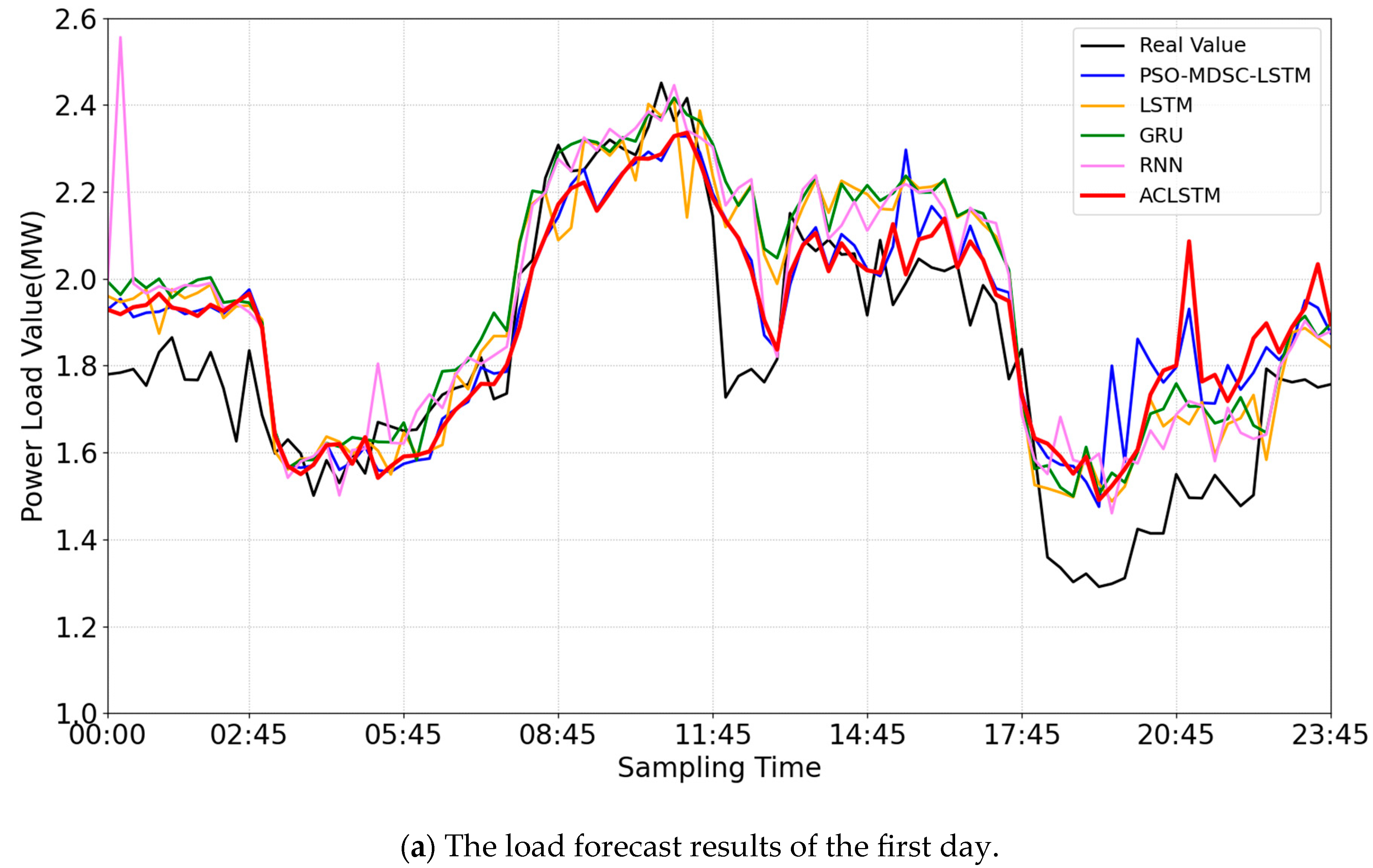
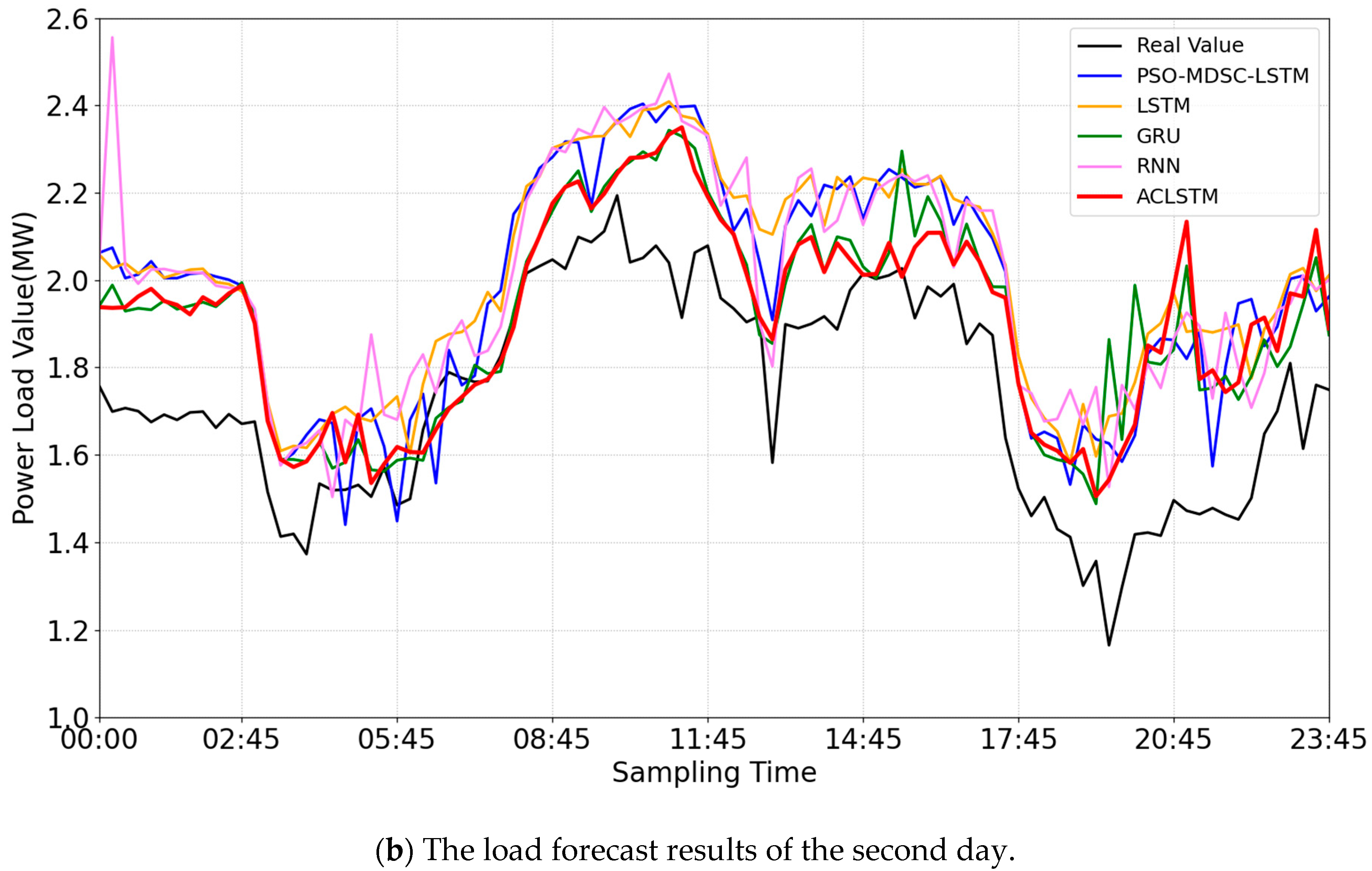
4.3.2. Experiment 2: Prediction Experiment

To evaluate the prediction performance of the algorithm proposed in this paper, an experiment is conducted using ACLSTM for power load forecasting over a two-day period. The results are compared with four other algorithms: PSO-MDSC-LSTM, LSTM [9], gated recurrent unit (GRU) [31], and recurrent neural network (RNN) [32]. PSO-MDSC-LSTM is the first algorithm that replaces BFLPSO in ACLSTM with traditional PSO while keeping the framework and parameters unchanged. The prediction results are presented in Figure 7 and

Table 2. Load prediction results.

Prediction	Statistical Project	ACLSTM	PSO-MDSC-LSTM	LSTM	RNN	GRU
the first day	MAPE(%)	8.05	8.21	8.27	8.18	8.55
	EMAX(%)	39.46	38.66	23.69	43.27	28.77
	EMIN(%)	0.30	0.07	0.09	0.02	0.55
	MAE	0.13	0.14	0.14	0.14	0.15
	MSE	0.03	0.03	0.03	0.03	0.03
	R2	0.65	0.63	0.65	0.60	0.63
the second day	MAPE(%)	11.45	11.61	14.67	15.60	16.32
	EMAX(%)	44.97	60.02	35.82	50.44	44.90
	EMIN(%)	0.12	0.06	0.09	0.40	4.88
	MAE	0.19	0.25	0.27	0.26	0.19
	MSE	0.05	0.07	0.08	0.08	0.05
	R2	0.12	−0.29	−0.49	−0.47	0.09

.

Based on Figure 7 and Table 2, the MAE, MSE, and R² values of ACLSTM and GRU show little difference. However, the MAPE of GRU is worse than that of ACLSTM. Specifically, for the second-day prediction, the MAPE of GRU is 16.32%, whereas ACLSTM only has a value of 11.45%. This represents an increase of 29.84% in MAPE for GRU compared to ACLSTM. Although LSTM and RNN yield better results for first-day predictions, the performance of RNN significantly deteriorates when predicting for the second day compared to ACLSTM. This is particularly evident in terms of MAPE, MAE, MSE, and R² values of RNN for the second-day prediction. The results obtained from PSO-MDSC-LSTM are similar to those achieved by ACLSTM. However, when it comes to predicting for the second day specifically, PSO-MDSC-LSTM performs much worse with an R² value of −0.29 compared to ACLSTM’s value of 0.12. It should be noted that a higher R² value indicates better prediction accuracy, whereas a negative value suggests poor prediction quality.

On the other hand, among the predicted load curves for the two days, ACLSTM demonstrates superior performance in terms of MAPE. Specifically, for the first-day prediction, ACLSTM achieves a MAPE of 8.05%, which is lower than PSO-MDSC-LSTM by 0.16%, LSTM by 0.22%, ANN by 0.15%, and GRU by 0.5%. The superiority of ACLSTM becomes even more apparent for the second-day prediction, with a MAPE that is lower than PSO-MDSC-LSTM by 0.16%, LSTM by 3.22%, ANN by 4.15%, and GRU by 4.87%.

ACLSTM outperforms the other four algorithms in terms of overall prediction stability, despite potentially having slightly larger errors for individual points. This demonstrates its effectiveness and superiority in power load forecasting, as it produces load curves that are much closer to the real data.

5. Conclusions

This paper presents ACLSTM, an algorithm for short-term load forecasting. ACLSTM combines BFLPSO and MDSC clustering to optimize parameters. BFLPSO’s spatial searching ability is utilized to find the best combinations of MDSC parameters. The algorithm uses 9-dimensional load feature vectors as training features for SVM, whereas the clustering results are used as labels to determine similarity clusters for forecast days. Load curves of two days are obtained using the LSTM neural network with similar clusters serving as training data. Comparison experiments demonstrate that BFLPSO-MDSC performs well in clustering, and the ACLSTM achieves higher prediction accuracy. The mean absolute percentage error for the first day is only 8.05% compared to the real value. These experiments validate the effectiveness, rationality, and practicality of ACLSTM. In future work, additional method comparison experiments should be conducted to provide further optimization ideas for this algorithm.

References

1. Papalexopoulos, A.D.; Hao, S.; Peng, T.M. An implementation of a neural network based load forecasting model for the EMS. IEEE Trans. Power Syst. 1994, 9, 1956–1962. [Google Scholar] [CrossRef]
2. Ma, H.; Xu, L.; Javaheri, Z.; Moghadamnejad, N.; Abedi, M. Reducing the consumption of household systems using hybrid deep learning techniques. Sustain. Comput. Inform. Syst. 2023, 38, 100874. [Google Scholar] [CrossRef]
3. Wang, B.; Wang, X.; Wang, N.; Javaheri, Z.; Moghadamnejad, N.; Abedi, M. Machine learning optimization model for reducing the electricity loads in residential energy forecasting. Sustain. Comput. Inform. Syst. 2023, 38, 100876. [Google Scholar] [CrossRef]
4. Kong, W.; Dong, Z.Y.; Hill, D.J.; Luo, F.; Xu, Y. Short-term residential load forecasting based on resident behaviour learning. IEEE Trans. Power Syst. 2018, 33, 1087–1088. [Google Scholar] [CrossRef]
5. Raza, M.Q.; Khosravi, A. A review on artificial intelligence based load demand forecasting techniques for smart grid and buildings. Renew. Sustain. Energy Rev. 2015, 50, 1352–1372. [Google Scholar] [CrossRef]
6. Coelho, V.N.; Coelho, I.M.; Coelho, B.N.; Reis, A.J.; Enayatifar, R.; Souza, M.J.; Guimarães, F.G. A self-adaptive evolutionary fuzzy model for load forecasting problems on smart grid environment. Appl. Energy 2016, 169, 567–584. [Google Scholar] [CrossRef]
7. Pulido, M.; Melin, P.; Castillo, O. Particle swarm optimization of ensemble neural networks with fuzzy aggregation for time series prediction of the Mexican Stock Exchange. Inf. Sci. 2014, 280, 188–204. [Google Scholar] [CrossRef]
8. Erdogdu, E. Electricity demand analysis using cointegration and ARIMA modelling. A case study of Turkey. Energy Policy 2007, 35, 1129–1146. [Google Scholar] [CrossRef]
9. Hong, W.C. Electric load forecasting by support vector model. Appl. Math. Model. 2009, 33, 2444–2454. [Google Scholar] [CrossRef]
10. Hochreiter, S.; Schmidhuber, J. Long short-term memory. Neural Comput. 1997, 9, 1735–1780. [Google Scholar] [CrossRef]
11. Kong, W.; Dong, Z.Y.; Jia, Y.; Hill, D.J.; Xu, Y.; Zhang, Y. Short-term residential load forecasting based on LSTM recurrent neural network. IEEE Trans. Smart Grid 2017, 10, 841–851. [Google Scholar] [CrossRef]
12. He, F.; Zhou, J.; Feng, Z.K.; Liu, G.; Yang, Y. A hybrid short-term load forecasting model based on variational mode decomposition and long short-term memory networks considering relevant factors with Bayesian optimization algorithm. Appl. Energy 2019, 237, 103–116. [Google Scholar] [CrossRef]
13. Li, J.; Deng, D.; Zhao, J.; Cai, D.; Hu, W.; Zhang, M.; Huang, Q. A novel hybrid short-term load forecasting method of smart grid using MLR and LSTM neural network. IEEE Trans. Ind. Inform. 2020, 17, 2443–2452. [Google Scholar] [CrossRef]
14. Fu, X.; Zeng, X.; Feng, P.; Cai, X. Clustering-based short-term load forecasting for residential electricity under the increasing-block pricing tariffs in China. Energy 2018, 165, 76–89. [Google Scholar] [CrossRef]
15. Sfetsos, A. Short-term load forecasting with a hybrid clustering algorithm. IEE Proc.-Gener. Transm. Distrib. 2003, 150, 257–262. [Google Scholar] [CrossRef]
16. Sander, J.; Ester, M.; Kriegel, H.P.; Xu, X. Density-based clustering in spatial databases: The algorithm gdbscan and its applications. Data Min. Knowl. Discov. 1998, 2, 169–194. [Google Scholar] [CrossRef]
17. Bian, H.; Zhong, Y.; Sun, J.; Shi, F. Study on power consumption load forecast based on K-means clustering and FCM–BP model. Energy Rep. 2020, 6, 693–700. [Google Scholar] [CrossRef]
18. Han, F.; Pu, T.; Li, M.; Taylor, G. Short-term forecasting of individual residential load based on deep learning and K-means clustering. CSEE J. Power Energy Syst. 2020, 7, 261–269. [Google Scholar]
19. Dong, X.; Deng, S.; Wang, D. A short-term power load forecasting method based on k-means and SVM. J. Ambient Intell. Humaniz. Comput. 2022, 13, 5253–5267. [Google Scholar] [CrossRef]
20. Gu, J.; Zhang, W.; Zhang, Y.; Wang, B.; Lou, W.; Ye, M.; Liu, T. Research on short-term load forecasting of distribution stations based on the clustering improvement fuzzy time series algorithm. CMES-Comput. Model. Eng. Sci. 2023, 136, 2221–2236. [Google Scholar] [CrossRef]
21. Zeng, W.; Li, J.; Sun, C.; Cao, L.; Tang, X.; Shu, S.; Zheng, J. Ultra short-term power load forecasting based on similar day clustering and ensemble empirical mode decomposition. Energies 2023, 16, 1989. [Google Scholar] [CrossRef]
22. Yang, W.; Shi, J.; Li, S.; Song, Z.; Zhang, Z.; Chen, Z. A combined deep learning load forecasting model of single household resident user considering multi-time scale electricity consumption behavior. Appl. Energy 2022, 307, 118197. [Google Scholar] [CrossRef]
23. Luo, Y.; Cai, Y.; Qi, Y. Short-term power load forecasting algorithm based on maximum deviation similarity criterion BP neural network. Appl. Res. Comput. 2019, 36, 3269–3273. [Google Scholar]
24. Niknam, T.; Amiri, B. An efficient hybrid approach based on PSO, ACO and k-means for cluster analysis. Appl. Soft Comput. 2010, 10, 183–197. [Google Scholar] [CrossRef]
25. Huang, J.; Xing, Y.; You, H.; Qin, L.; Tian, J.; Ma, J. Particle swarm optimization-based noise filtering algorithm for photon cloud data in forest area. Remote Sens. 2019, 11, 980. [Google Scholar] [CrossRef]
26. Perafan-Lopez, J.C.; Ferrer-Gregory, V.L.; Nieto-Londoño, C.; Sierra-Pérez, J. Performance analysis and architecture of a clustering hybrid algorithm called FA+ GA-DBSCAN using artificial datasets. Entropy 2022, 24, 875. [Google Scholar] [CrossRef] [PubMed]
27. Chen, X.; Tianfield, H.; Du, W. Bee-foraging learning particle swarm optimization. Appl. Soft Comput. 2021, 102, 107134. [Google Scholar] [CrossRef]
28. Van den Bergh, F.; Engelbrecht, A.P. A cooperative approach to particle swarm optimization. IEEE Trans. Evol. Comput. 2004, 8, 225–239. [Google Scholar] [CrossRef]
29. Hassan, R.; Cohanim, B.; De Weck, O.; Venter, G. A comparison of particle swarm optimization and the genetic algorithm. In Proceedings of the 46th AIAA/ASME/ASCE/AHS/ASC Structures, Structural Dynamics and Materials Conference, Austin, TX, USA, 18–21 April 2005. [Google Scholar]
30. Luo, Y.; Cai, Y.; Qi, Y.; Chen, H.; Wang, S. Long short-term power load forecasting algorithm using long short-term memory neural network with density-based spatial clustering. In Proceedings of the 2019 IEEE 5th International Conference on Computer and Communications (ICCC), Chengdu, China, 6–9 December 2019. [Google Scholar]
31. Jia, T.; Yao, L.; Yang, G.; He, Q. A short-term power load forecasting method of based on the CEEMDAN-MVO-GRU. Sustainability 2022, 14, 16460. [Google Scholar] [CrossRef]
32. Medina-Santana, A.A.; Cárdenas-Barrón, L.E. Optimal design of hybrid renewable energy systems considering weather forecasting using recurrent neural networks. Energies 2022, 15, 9045. [Google Scholar] [CrossRef]
Figure 1. The flowchart of BFLPSO-MDSC.
Energies 16 06230 g001
Figure 2. The flowchart of ACLSTM.
Energies 16 06230 g002
Figure 3. Clustering results of BFLPSO-MDSC.
Energies 16 06230 g003
Figure 4. Clustering results of PSO-MDSC.
Energies 16 06230 g004
Figure 5. Clustering results of DBSCAN.
Energies 16 06230 g005
Figure 6. Clustering results of K-Means.
Energies 16 06230 g006
Figure 7. Comparison of load prediction results of five algorithms.
Energies 16 06230 g007aEnergies 16 06230 g007b