Robust Multiobjective Decision Making in the Acquisition of Energy Assets

Abstract

In asset management for energy portfolios, quantitative methodologies are typically employed. In Brazil, the NEWAVE computational model is universally used to generate scenarios of hydraulic production and future prices, which result in revenue distributions. These distributions are then used to estimate the portfolio’s revenue and assess its risk. Although this is a well-established analysis, it has some shortcomings that are not always considered. The validity of the revenue series constructed by NEWAVE, especially in long-term analysis, is a real problem for agents concerning the acquisition of assets such as power plants. Another issue is the disregard for other objectives that are important for the operationality of the management task and are often ignored, such as operational risk. To address these limitations, this work combines the areas of multicriteria decision making under uncertainty and risk management and presents a methodology for evaluating the acquisition of long-term energy assets, as well as a practical application of the proposed method. Investment alternatives are evaluated in multiple developed scenarios, so it is possible to measure how robust a given option is. By analyzing several scenarios simultaneously, a larger region of uncertainties can be covered, and therefore, decision making becomes more secure. The proposed methodology includes six objectives, designed to address a wider range of stakeholder needs. This approach is applied to an illustrative portfolio, producing results that allow for a more comprehensive understanding of decision attributes. Therefore, this work not only addresses the current limitations in the field but also adds an original contribution by considering simultaneously several scenarios and integrating multiple objectives in a robust and secure decision-making framework.

1. Introduction

Electric power is a commodity with high volatility and uncertainty in its price. With the evolution of energy markets, the possibility was created for market agents to freely trade this commodity. This fact makes markets more dynamic and competitive [1,2]. With the changes in the electric sector and advances in opening the energy market, which led to an increase in the number of transactions, agents realized that efficient risk management is essential for the healthy performance of this activity [3].

Risk analysis is strategically important as it is necessary to identify factors that will influence the financial return of an investment [4]. The acquisition of new energy assets by a generating agent cannot be decided solely based on their costs, whether investment or generation, as it is an activity with long-term impacts. During decision making about a change in the portfolio, risks of different natures are to be considered [5,6,7].

To define a portfolio, market participants adhere to two objective functions: maximizing the expected net revenue of the portfolio (E[NPV]) and maximizing revenue in the worst scenarios (written through the conditional value at risk (CVaR)) [8,9]. The use of revenue at risk (RaR) as an operational limit is also common, in an attempt to control the size of revenue dispersion. However, other ways of measuring risk could be used, such as the lower partial moments used in [10] or the cash flow at risk approach presented in [6].

An important point in decision making under conditions of uncertainty is the absence of optimal solutions (regardless of whether the problem is monocriteria or multicriteria): the solution optimal for one scenario is not optimal for another scenario. So, what is a decision under conditions of uncertainty? The solution under conditions of uncertainty is a robust (or non-dominated) solution, which permits one to attend any scenario in the best way [11]. How is it possible to find a robust solution? The discipline of Operations Research cannot help her. It is based on the concept of existing optimal solutions. All approaches, methods and strategies of Operations Research are directed at obtaining optimal solutions, which do not exist. Considering this, a strategy applied in this work is directed at finding the worst solutions, which are dominated by other solutions. By cutting off the worst solutions and applying any type of preference information, it is possible to reduce decision uncertainty regions.

This paper proposes an evolution of a methodological inheritance for the selection of energy portfolios. The Brazilian energy market operates and is oriented towards a periodic autoregressive model used by the National System Operator for its control and operation [12]. In turn, other market participants also use this tool for their commercial and operational risk management. However, due to the characteristics of the sector, the price and generation forecasts returned by this system are sensitive to initial conditions and climate forecasts. This sensitivity can influence the accuracy of the model’s result, and relying on a single forecast may not be sufficient for decision making.

Therefore, the objective of this work is to use the decision-making techniques proposed in [11,13] for the construction of portfolios and their analysis in multiple scenarios. To achieve this, the performance of an agent’s portfolio in different constructed scenarios was evaluated. This performance is assessed by applying the $〈X,F〉$ decision-making model [11,13] using the functions of expected net present value, CVaR, and revenue at risk, which are already used by the market. This article also proposes the use of new objective functions—insurance index (InS), alternative synergy with the current portfolio and operational risks—in addition to the classical objective functions for making decisions on energy portfolios. By stressing the cases and using decision-making methodologies, it is possible to construct a robust portfolio for the company’s position.

Characterizing the originality and contribution of this work, it is necessary to stress that the majority of methods related to energy trade and portfolio management are based on the probabilistic approach [14]. However, it is not possible to talk about the future and construct the future based on past information and trends, at least for long-term planning (as evident from events such as the global financial crisis of 2008 and the COVID pandemic in 2020). Considering this, in the present work, we try to use the possibilistic approach, which consists in constructing and using representative combinations of initial data, states of nature, or scenarios. This work proposes the use of six objective functions, designed specifically to address the unique demands of agents engaged in asset acquisition during the process of energy portfolio management.

The paper is structured as follows. Section 2 presents a review of correlated works and theoretical references. Section 3 describes the proposed method and objective functions. Section 4 presents the characteristics of the problem, the problem formulation, the initial data, and the evaluated alternatives. The results of this paper are illustrated by considering a case study given in Section 5. Finally, in Section 6, the main conclusions of this study are presented.

2. Theoretical Reference

2.1. Private Investments in Energy

In the context of energy market operations, companies buy and sell energy to manage their energy balance over time and ensure their operational stability while seeking the lowest possible cost. To improve the way they perform this task, companies have started applying financial risk management models and began trading energy based on a multicriteria approach, considering revenues and market risks directly in the construction of their energy portfolios.

Considering that this work, from a practical application perspective, is dedicated to the risk management of energy portfolios, it is necessary to indicate the results of [2,3,5,6]. These works can be considered as the initial theoretical bases of the discussion of the problem of risk management in energy portfolios, which continues today. These works present the reason why energy prices are volatile parameters and discuss financial engineering approaches to measuring risks in the energy market.

The results presented in [2] addressed the modeling of the risk metric value at risk (VaR). The authors of [2] explain how the methodology should be used, presenting requirements such as return forecasts. The VaR metric is also addressed in [5], as well as CVaR and other metrics. It exposes some examples and comparisons of results from the used methods. In [6], different risk metrics are presented, and how market risks can be measured and managed using real options models and stochastic optimization techniques is explored. Moreover, in [3], there is a discussion about how energy prices can fluctuate and the associated risks when pricing and hedging electricity derivatives.

Regarding trading, in general, agents seek commercial strategies that contemplate seasonal productions of each source at each period of the year, in order to offer the best negotiation. The work of Camargo et al. [15] deals with the management of energy trading contracts through the formation of portfolios composed of renewable energy sources, from the point of view of the generator, consumer, and trader. From the generator’s perspective, this work analyzes risk management policies defined based on the periodic accounting of CVaR and their influence on contracting strategies. Additionally, this work explores how Swap contracts are used to provide security for parties during times when the short-term market is vulnerable, given the conditions of purchase and sale prices, the hydraulic generator’s contractual balance, the agent’s risk aversion, and the projections of the settlement price for differences (Preço de Liquidação das Diferenças (PLD)) and generation scaling factor (GSF) in the planning horizon.

To define these projections in the Brazilian market, agents use a computational model called NEWAVE. However, since it is a tool undergoing constant changes, using it as the only reference in decision making can be inadequate [12]. The fact that the electrical system undergoes constant regulatory evolutions and the use of new technologies can also invalidate these projections in the long term [16].

In order to address the limitations of conventional risk assessment methods, the work of Ilbahar et al. [17] incorporates the subjective judgment of decision makers to map uncertainties in the risk factors of renewable energy projects. Overall, the paper presents a new and comprehensive approach to assessing risks in renewable energy investments that overcomes the limitations of traditional methods. However, the proposed approach may require a higher level of expertise and effort in data collection and analysis, which may limit its practical application in some contexts.

Another work dealing with decision making in energy investments is [18]. This work proposes an approach that combines a fuzzy analytical hierarchy process (FAHP) and a technique for order preference by similarity to the ideal solution (TOPSIS) to assess the suitability of new potential services in the renewable energy sector. The challenges and complexities associated with the process of developing new services in the renewable energy sector are also discussed, including technological uncertainty and the need for collaboration among stakeholders.

On the same path, the authors of [19] propose a stochastic decision support model for renewable energy investments in Brazil that considers expected returns and CVaR as objective functions and NEWAVE output data for scenario creation. The study reveals that the risk associated with intermittent sources can be managed through CVaR assessments, although the level of the decision maker’s risk aversion significantly influences the company’s market position. The authors found that a diversified firm’s asset base, along with the complementary nature of generation sources, can significantly reduce the financial risks of the investor’s portfolio. These results showed that the decision of a new investment must consider the current portfolio of the company.

Recent studies discussing multiobjective decision making in energy trading also include works [20,21]. The authors of [20] propose a hybrid trading mechanism that operates on multiple time scales, taking into account the transmission speeds and limits of various energy sources, while developing a strategy based on the Markov decision process. On the other hand, the authors of [21] explore energy trading strategies in a residential energy system. Although both studies present strategies that improve energy costs for the involved agents, these studies tend to overlook other needs of the agents, thereby compromising the construction of a robust portfolio. Additionally, they focus on short-term analysis, which may limit the comprehensiveness and real-world applicability of their strategies.

When making long-term decisions, it is essential to consider the uncertainty and variability of the future. This is where possibilistic information becomes crucial. Unlike probabilistic information, which relies on statistical analysis and provides the likelihood of certain outcomes occurring, possibilistic information considers the uncertainty of the future and focuses on the range of possible outcomes without assigning probabilities [11]. This is necessary since the future is constantly evolving, with regulatory, technological, and other changes constantly altering the range of possible outcomes, and is what makes this work different from those mentioned above. Therefore, decision makers should be aware that probabilities can quickly become outdated and should be prepared to adapt their plans accordingly. In this sense, a possibilistic view of decision making, focusing on the range of possible outcomes instead of assigning probabilities, may be more reliable in the long term [22].

According to [23], to account for the revenue of an energy portfolio, let W be the set of energy assets. It follows that $x_{i,t}\in W$ is the volume resulting from the purchase (or sale, if negative) of an energy asset i in period t. Therefore, the result (revenue or expense) of trading an energy asset can be described as follows:

$${\varrho }_t^E\left(x_t\right)=h_t\left(\sum _{c=1}^C{p}_{c,t}{v}_{c,t}+\sum _{i=1}^I{p}_{i,t}{x}_{i,t}\right),\forall i\in W_c,$$

(1)

where $h_t$ is the number of hours within period t, $W_c$ is the set of assets that are energy contracts, C is the total number of contracts, I is the total number of assets of a certain type, v is the volume of energy bought/sold already existing in the portfolio, and p is the price of the contract/asset.

The operation and maintenance cost of the agent’s assets can be described as:

$${\varrho }_{t,s}^M\left(x_t\right)=h_t\sum _{i=1}^I\left(-{\theta }_i\left(g_{i,t,s}+x_{i,t}\right)\right),\forall i\in W\wedge \neg W_c,$$

(2)

where ${\theta }_i$ is the operation and maintenance cost of the plant, modeled by a constant whose unit is expressed in $R$$/MWh, and $g_{i,t,s}$ is the volume of energy existing in the portfolio.

The revenue, or expense, resulting from energy exposed to the spot market can be described as:

$${\varrho }_{t,s}^P\left(x_t\right)=h_{t}PL{D}_{t,s}{\xi }_{t,s}\left(x_t\right),$$

(3)

where the energy exposure to the short-term market is calculated as follows:

$${\xi }_{t,s}\left(x_t\right)=\sum _{i=1}^I{\gamma }_{t,s}·x_{i,t}+\sum _{i=1}^I\tilde{g}i,t,s+\widehat{V}t,s-{\check{V}}_{t,s}.$$

(4)

In (4), ${\gamma }_{t,s}$ equals 1 for all assets, except for hydraulics, participating in the MRE, since $\gamma$ is the generation scaling factor (GSF). The ${\tilde{g}}_{i,t,s}$ is the adjusted physical guarantee of the agent, if the asset is hydraulic plants participating in the MRE, since in this case, the resource considered for the plant is its physical guarantee multiplied by the GSF factor. The physical guarantee value, in general, defines the maximum amount of energy that the project can trade [23].

The total volumes resulting from energy purchase or sale contracts are represented by the terms ${\widehat{V}}_{t,s}$ and ${\check{V}}_{t,s}$, respectively. In other words, the portion that composes the exposure result consists of the balance value between the resource and the requirement.

Therefore, the total revenue of an agent with multiple assets of different types can be defined by the following equation:

$${\varrho }_{t,s}\left(x_t\right)={\varrho }_t^E\left(x_t\right)+{\varrho }_{t,s}^M\left(x_t\right)+{\varrho }_{t,s}^P\left(x_t\right).$$

(5)

Since this is a long-term investment evaluation approach, seasonality and energy modulation, practices used by the Brazilian market agents for portfolio operation in monthly and daily time frames, will not be considered.

2.2. Generalization of the Classical Approach to Dealing with Information Uncertainty

The classical approach [24,25,26] for dealing with information uncertainty is based on the assumption that the analysis is carried out for a given number K of solution alternatives $X_k,k=1,\dots ,K$ and a given number J of representative combinations of initial data (the states of nature or scenarios) $Y_j,j=1,\dots ,J$, which define the corresponding payoff matrix. The payoff matrix, presented in

Table 1. Payoff matrix with characteristics estimates.

	${\mathit{Y}}_1$	$\dots$	${\mathit{Y}}_{\mathit{j}}$	$\dots$	${\mathit{Y}}_{\mathit{J}}$	${\mathit{F}}^{\mathit{min}}\left({\mathit{X}}_{\mathit{k}}\right)$	${\mathit{F}}^{\mathit{max}}\left({\mathit{X}}_{\mathit{k}}\right)$	$\overline{\mathit{F}}\left({\mathit{X}}_{\mathit{k}}\right)$	${\mathit{R}}^{\mathit{max}}\left({\mathit{X}}_{\mathit{k}}\right)$
$X_1$	$F(X_1,Y_1)$	$\dots$	$F(X_1,Y_j)$	$\dots$	$F(X_1,Y_J)$	$F^{min}\left(X_1\right)$	$F^{max}\left(X_1\right)$	$\overline{F}\left(X_1\right)$	$R^{max}\left(X_1\right)$
$\dots$	$\dots$	$\dots$	$\dots$	$\dots$	$\dots$	$\dots$	$\dots$	$\dots$	$\dots$
$X_k$	$F(X_k,Y_1)$	$\dots$	$F(X_k,Y_j)$	$\dots$	$F(X_k,Y_J)$	$F^{min}\left(X_k\right)$	$F^{max}\left(X_k\right)$	$\overline{F}\left(X_k\right)$	$R^{max}\left(X_k\right)$
$\dots$	$\dots$	$\dots$	$\dots$	$\dots$	$\dots$	$\dots$	$\dots$	$\dots$	$\dots$
$X_K$	$F(X_K,Y_1)$	$\dots$	$F(X_K,Y_j)$	$\dots$	$F(X_K,Y_J)$	$F^{min}\left(X_K\right)$	$F^{max}\left(X_K\right)$	$\overline{F}\left(X_K\right)$	$R^{max}\left(X_K\right)$

Source: [22].

(the first six columns), reflects the effects (or consequences) of an action $X_k$ for the corresponding state of nature.

The analysis of payoff matrices and the choice of rational solution alternatives are based on the use of choice criteria [24,25,26]. The application of the choice criteria of Wald, Laplace, Savage, and Hurwicz, which are of a general nature, is discussed next. There are other choice criteria, for example, Bayes, maximum probability, minimum dispersion, maximum measure of Bayesian sets, maximum integral power, etc. [27,28]. However, these criteria assume certain informational situations about the states of nature.

To better understand the use of the criteria of Wald, Laplace, Savage, and Hurwicz, Table 1 includes the following characteristics estimates for a solution alternative:

• The minimum level of objective function:

  $$F^{min}\left(X_k\right)=\underset{1\le j\le J}{\min }F(X_k,Y_j),$$

  (6)

  which is the most optimistic estimate if the objective function is to be minimized or the most pessimistic estimate if the objective function is to be maximized;
• The maximum level of objective function:

  $$F^{max}\left(X_k\right)=\underset{1\le j\le J}{\max }F(X_k,Y_j),$$

  (7)

  which is the most optimistic estimate for the maximized objective function or the most pessimistic estimate if the objective function is to be minimized;
• The average level of objective function:

  $$\overline{F}\left(X_k\right)=\frac{1}{J}\sum _{j=1}^{J}F(X_k,Y_j);$$

  (8)
• The maximum level of regret:

  $$R^{max}\left(X_k\right)=\underset{1\le j\le J}{\max }R(X_k,Y_j),$$

  (9)

  where $R\left(X_k,Y_j\right)$ is an excess of expenses that occur under the combination of the state of nature $Y_j$ and the choice of the solution alternative $X_k$ instead of the solution alternative that is locally optimal for the given $Y_j$.

To determine the regrets $R(X_k,Y_j)$, it is necessary to define the minimum value of the objective function for each combination of the state of nature:

$$F^{min}\left(Y_j\right)=\underset{1\le k\le K}{\min }F(X_k,Y_j).$$

(10)

On the other hand, if the objective function is to be maximized, it is necessary to define its maximum value for each combination of the state of nature (for each column of the payoff matrix):

$$F^{max}\left(Y_j\right)=\underset{1\le k\le K}{\max }F(X_k,Y_j).$$

(11)

The regret for any alternative solution $X_k$ and any state of nature $Y_j$ can be assessed as:

$$R(X_k,Y_j)=F(X_k,Y_j)-F^{min}\left(Y_j\right),$$

(12)

if the objective function is to be minimized, or

$$R(X_k,Y_j)=F^{max}\left(Y_j\right)-F(X_k,Y_j),$$

(13)

if the objective function is to be maximized.

The choice criteria, based on the use of characteristic estimates, are represented as (14)–(17) under the assumption that the objective function is to be minimized. The Wald choice criterion uses the estimate $F^{max}\left(X_k\right)$ and allows choosing the solution alternatives $X^W$, for which the estimate is minimum:

$$\underset{1\le k\le K}{\min }{F}^{max}\left(X_k\right)=\underset{1\le k\le K}{\min }\underset{1\le j\le J}{\max }F(X_k,Y_j).$$

(14)

The use of this criterion generates solution alternatives, assuming the most unfavorable combination of initial data. It ensures that the level of the objective function is not greater than a certain value under any possible future conditions. On the other hand, the focus on the most unfavorable combination of initial data is extremely cautious (pessimistic or conservative) [26].

The Laplace choice criterion, $\overline{F}\left(X_k\right)$, uses the estimate (8) and is aimed at choosing the solution alternatives $X^L$, for which the estimate is minimum:

$$\underset{1\le k\le K}{\min }\overline{F}\left(X_k\right)=\underset{1\le k\le K}{\min }\frac{1}{J}\sum _{j=1}^{J}F(X_k,Y_j).$$

(15)

This criterion corresponds to the principle of “insufficient reason” [26], that is, the assumption that we have no basis for distinguishing a particular combination of initial data. Therefore, it is necessary to act as if they are equally likely, which is a disadvantage. However, the average score is sufficiently important.

The Savage choice criterion is associated with the use of the estimate $R^{max}\left(X_k\right)$ and allows choosing the solution alternatives $X^S$, for which the estimate is minimum:

$$\underset{1\le k\le K}{\min }{R}^{max}\left(X_k\right)=\underset{1\le k\le K}{\min }\underset{1\le j\le J}{\max }R(X_k,Y_j).$$

(16)

As in the case of the Wald choice criterion, the use of Equation (16) is based on the $minmax$ principle. Therefore, the Savage choice criterion can also be considered conservative. However, the experience of [26] shows that the recommendations based on the application of Equation (16) can be inconsistent with the decisions obtained with the use of Equation (14). Operating with values of $R^{max}\left(X_k\right)$, we obtain a slightly different assessment of the situation, which could lead to more “daring” (less conservative) recommendations.

Finally, the Hurwicz choice criterion uses a convex combination of $F^{max}\left(X_k\right)$ and $F^{min}\left(X_k\right)$ and allows choosing the solution alternatives $X^H$ that produce the minimum for:

$$\underset{1\le k\le K}{\min }\left(\beta F^{max}\left(X_k\right)+(1-\beta )F^{min}\left(X_k\right)\right)=\underset{1\le k\le K}{\min }\left(\beta \underset{1\le j\le J}{\max }F(X_k,Y_j)+(1-\beta )\underset{1\le j\le J}{\min }F(X_k,Y_j)\right),$$

(17)

where $\beta \in \left[0,1\right]$ is the “pessimism–optimism” index whose magnitude is defined by the decision maker. If $\beta =1$, the Hurwicz choice criterion is transformed into the Wald choice criterion, and if $\beta =0$, Equation (17) is transformed into the criterion of “extreme optimism” ($minmin$) for which the combination of initial data is most favorable. The author of [26] recommends choosing a range of $0.5<\beta <1$.

The choice criteria discussed above have found widespread practical applications, as in [26,29] in both mono-objective and multiobjective problems.

The definition of the solution alternatives can be based on applying the modification [30] of the Bellman–Zadeh approach to decision making in a fuzzy environment [31]. This approach is used for solving multiobjective problems for each scenario, with the modification providing constructive lines for obtaining harmonious solutions to such problems [32]. These solution alternatives, also referred to as locally optimal solution alternatives, serve as the basis for constructing the payoff matrices. Nonetheless, in some instances, the decision makers themselves may also propose solutions for constructing these matrices, such as in this paper.

The generalization of the classical approach to dealing with information uncertainty [11,32,33] is associated with the analysis of the problems defined by Equations (14)–(17) for a given objective function in an environment with multiple states of nature $Y_j,j=1,\dots ,J$. Therefore, considering the Wald, Laplace, Savage, and Hurwicz choice criteria, respectively, as objective functions, we consider:

$$F^W\left(X_k\right)=F^{min}\left(X_k\right)=\underset{1\le j\le J}{\min }F(X_k,Y_j),$$

(18)

$$F^L\left(X_k\right)=\overline{F}\left(X_k\right)=\frac{1}{J}\sum _{j=1}^{J}F(X_k,Y_j),$$

(19)

$$F^S\left(X_k\right)=R^{max}\left(X_k\right)=\underset{1\le j\le J}{\max }R(X_k,Y_j),$$

(20)

$$F^H\left(X_k\right)=\beta F^{max}\left(X_k\right)+(1-\beta )F^{min}\left(X_k\right)=\beta \underset{1\le j\le J}{\max }F(X_k,Y_j)+(1-\beta )\underset{1\le j\le J}{\min }F(X_k,Y_j).$$

(21)

This consideration of the choice criteria allows constructing q problems that generally include four or fewer objective functions (if not all choice criteria are used in the analysis) as follows:

$$F_{r,p}\left(X\right)\to \underset{X\in L}{\mathrm{extr}},r=1,\dots ,t\le 4,p=1,\dots ,q,$$

(22)

where L represents the feasible region for choosing solutions.

Thus, the analysis of solution alternatives and consequent choice of rational solution alternatives can be carried out within the $〈X,F〉$ models [11,13,33].

The analysis, performed in this way, ensures the choice of rational solution alternatives according to the principle of Pareto optimality [32]. Considering this, the payoff matrix with characteristic estimates, presented in Table 1, is transformed into the matrix of choice criteria estimates in

Table 2. Matrix with the choice criteria for the objective function of number p.

	${\mathit{F}}_{\mathit{p}}^{\mathit{W}}\left({\mathit{X}}_{\mathit{k}}\right)$	${\mathit{F}}_{\mathit{p}}^{\mathit{L}}\left({\mathit{X}}_{\mathit{k}}\right)$	${\mathit{F}}_{\mathit{p}}^{\mathit{S}}\left({\mathit{X}}_{\mathit{k}}\right)$	${\mathit{F}}_{\mathit{p}}^{\mathit{H}}\left({\mathit{X}}_{\mathit{k}}\right)$
$X_1$	$F_p^W\left(X_1\right)$	$F_p^L\left(X_1\right)$	$F_p^S\left(X_1\right)$	$F_p^H\left(X_1\right)$
$\dots$	$\dots$	$\dots$	$\dots$	$\dots$
$X_k$	$F_p^W\left(X_k\right)$	$F_p^L\left(X_k\right)$	$F_p^S\left(X_k\right)$	$F_p^H\left(X_k\right)$
$\dots$	$\dots$	$\dots$	$\dots$	$\dots$
$X_K$	$F_p^W\left(X_k\right)$	$F_p^L\left(X_k\right)$	$F_p^S\left(X_k\right)$	$F_p^H\left(X_k\right)$
	$\underset{1\le k\le K}{\min }{F}_p^W\left(X_k\right)$	$\underset{1\le k\le K}{\min }{F}_p^L\left(X_k\right)$	$\underset{1\le k\le K}{\min }{F}_p^S\left(X_k\right)$	$\underset{1\le k\le K}{\min }{F}_p^H\left(X_k\right)$
	$\underset{1\le k\le K}{\max }{F}_p^W\left(X_k\right)$	$\underset{1\le k\le K}{\max }{F}_p^L\left(X_k\right)$	$\underset{1\le k\le K}{\max }{F}_p^S\left(X_k\right)$	$\underset{1\le k\le K}{\max }{F}_p^H\left(X_k\right)$

Source: [33].

.

Therefore, using q matrices for the estimates of the choice criteria, we can construct q modified matrices of the choice criteria estimates, as shown in

Table 3. Matrix with the modified choice criteria for the objective function of number p.

	${\mathit{\mu }}_{{\mathit{A}}_{\mathit{p}}}^{\mathit{W}}\mathsf{(}{\mathit{X}}_{\mathit{k}}\mathsf{)}$	${\mathit{\mu }}_{{\mathit{A}}_{\mathit{p}}}^{\mathit{L}}\mathsf{(}{\mathit{X}}_{\mathit{k}}\mathsf{)}$	${\mathit{\mu }}_{{\mathit{A}}_{\mathit{p}}}^{\mathit{S}}\mathsf{(}{\mathit{X}}_{\mathit{k}}\mathsf{)}$	${\mathit{\mu }}_{{\mathit{A}}_{\mathit{p}}}^{\mathit{H}}\mathsf{(}{\mathit{X}}_{\mathit{k}}\mathsf{)}$
$X_1$	${\mu }_{A_p}^W\left(X_1\right)$	${\mu }_{A_p}^L\left(X_1\right)$	${\mu }_{A_p}^S\left(X_1\right)$	${\mu }_{A_p}^H\left(X_1\right)$
$\dots$	$\dots$	$\dots$	$\dots$	$\dots$
$X_k$	${\mu }_{A_p}^W\left(X_k\right)$	${\mu }_{A_p}^L\left(X_k\right)$	${\mu }_{A_p}^S\left(X_k\right)$	${\mu }_{A_p}^H\left(X_k\right)$
$\dots$	$\dots$	$\dots$	$\dots$	$\dots$
$X_K$	${\mu }_{A_p}^W\left(X_k\right)$	${\mu }_{A_p}^L\left(X_k\right)$	${\mu }_{A_p}^S\left(X_k\right)$	${\mu }_{A_p}^H\left(X_k\right)$

Source: [33].

, by applying the relations:

$${\mu }_{A_p}\left(X\right)={\left(\frac{\underset{X\in L}{\max }{F}_p\left(X\right)-F_p\left(X\right)}{\underset{X\in L}{\max }{F}_p\left(X\right)-\underset{X\in L}{\min }{F}_p\left(X\right)}\right)}^{{\lambda }_p},$$

(23)

for the objective functions that must be minimized and relations:

$${\mu }_{A_p}\left(X\right)={\left(\frac{F_p\left(X\right)-\underset{X\in L}{\min }{F}_p\left(X\right)}{\underset{X\in L}{\max }{F}_p\left(X\right)-\underset{X\in L}{\min }{F}_p\left(X\right)}\right)}^{{\lambda }_p},$$

(24)

for the objective functions that must be maximized. In (23) and (24), ${\mu }_{A_p}$ is the membership function of the p-th objective function, and ${\lambda }_p$ is the importance coefficient of the p-th objective function.

Finally, in the presence of q modified matrices of the choice criteria estimates, applying the results from [11,33], we can construct the aggregated matrix of the choice criteria estimates, as shown in

Table 4. Matrix with the aggregated levels of the fuzzy choice criteria.

	${\mathit{\mu }}_{\mathit{D}}^{\mathit{W}}\mathsf{(}{\mathit{X}}_{\mathit{k}}\mathsf{)}$	${\mathit{\mu }}_{\mathit{D}}^{\mathit{L}}\mathsf{(}{\mathit{X}}_{\mathit{k}}\mathsf{)}$	${\mathit{\mu }}_{\mathit{D}}^{\mathit{S}}\mathsf{(}{\mathit{X}}_{\mathit{k}}\mathsf{)}$	${\mathit{\mu }}_{\mathit{D}}^{\mathit{H}}\mathsf{(}{\mathit{X}}_{\mathit{k}}\mathsf{)}$
$X_1$	${\mu }_D^W\left(X_1\right)$	${\mu }_D^L\left(X_1\right)$	${\mu }_D^S\left(X_1\right)$	${\mu }_D^H\left(X_1\right)$
$\dots$	$\dots$	$\dots$	$\dots$	$\dots$
$X_k$	${\mu }_D^W\left(X_k\right)$	${\mu }_D^L\left(X_k\right)$	${\mu }_D^S\left(X_k\right)$	${\mu }_D^H\left(X_k\right)$
$\dots$	$\dots$	$\dots$	$\dots$	$\dots$
$X_K$	${\mu }_D^W\left(X_k\right)$	${\mu }_D^L\left(X_k\right)$	${\mu }_D^S\left(X_k\right)$	${\mu }_D^H\left(X_k\right)$
	$\underset{1\le k\le K}{\max }{\mu }_D^W\left(X_k\right)$	$\underset{1\le k\le K}{\max }{\mu }_D^L\left(X_k\right)$	$\underset{1\le k\le K}{\max }{\mu }_D^S\left(X_k\right)$	$\underset{1\le k\le K}{\max }{\mu }_D^H\left(X_k\right)$

Source: [33].

. This matrix includes the estimates calculated based on [11] and can be used to select non-dominated or robust solution alternatives.

Where ${\mu }_D$ is the aggregated membership function, which is obtained using the minimum operator. Taking into account the results presented above, it is possible to suggest the general scheme of multicriteria decision making under conditions of information uncertainty that is associated with the following steps, in the general case:

• The first step involves constructing q payoff matrices, corresponding to the number of objective functions. These matrices account for all combinations of solution alternatives $X_k,k=1,\dots ,K$ and the representative states of nature $Y_j,j=1,\dots ,J$. To construct payoff matrices, it is necessary to solve q multicriteria problems formalized within the framework of $〈X,F〉$ models. By solving them, it is possible to obtain the solution alternatives $X_k,k=1,\dots ,K$ ($K\le J$). After that, $X_k,k=1,\dots ,K$ are substituted $F_p\left(X\right),p=1,\dots ,q$ for $Y_j,j=1,\dots ,J$. These substitutions generate q payoff matrices;
• The second step is related to the analysis of the obtained payoff matrices. The execution of this phase is based on the approach proposed in [11] discussed above. However, the insufficient resolving capacity of this phase may lead to non-unique or not well-distinguished solutions, and this circumstance demands the application of the third phase;
• The third step is associated with the construction and analysis of $〈X,R〉$ models [11,22] for the subsequent contraction of decision uncertainty regions. The use of $〈X,R〉$ models allows taking into account indices of quantitative character and qualitative character, based on the knowledge, experience, and intuition of the involved experts

2.3. $\langle X,R\rangle$ Decision-Making Models

Decision-making models based on qualitative information are a type of decision-making tool that relies on non-numerical information to evaluate, compare, select, order, and/or prioritize solution alternatives on the basis of the corresponding preferences of decision makers. These models are particularly useful when there is a lack of reliable data or when the decision encounters complex or ambiguous situations. One of the main features of decision-making models that use qualitative information is that they rely on subjective judgments and opinions, rather than objective data. These models permit one to include things such as personal experience, specialized knowledge, and intuition. Although this may seem less reliable than quantitative data, qualitative information can be invaluable in situations where there are no reliable data available or where the decision is based on human behavior, emotions, or beliefs [34].

Another feature of qualitative information-based decision-making models is that they are often used in situations where the decision maker faces uncertainty or ambiguity of information. One of the advantages of qualitative decision-making models is that they can be more flexible than quantitative models. Since they do not rely on specific numerical data, they can be adapted to suit different situations and circumstances. This can be particularly useful when making decisions in dynamic or changing environments, where data may be incomplete or unreliable [35].

Moreover, many situations requiring the application of the multicriteria approach are associated with the problems that can initially be solved based on a single criterion or multiple criteria. However, if the uncertainty of information does not allow defining a unique solution, it is possible to use additional criteria to distinguish the alternatives.

There exist diverse formats of preference representation, as discussed, for instance, in [22]. Taking this into account, it is necessary to indicate that the results of [13] permit one to transform different formats as well as information of qualitative character to non-reciprocal fuzzy preference relations, applying so-called transformation functions. It allows us to concentrate attention on procedures of decision making in a fuzzy environment.

Suppose there is a set X of alternatives coming from the decision uncertainty region and/or predetermined alternatives, which are to be evaluated on q criteria. The decision-making problem can be presented by the pair $\langle X,R\rangle$ where $R=\left\{R_1,R_2,\dots ,R_p,\dots ,R_q\right\}$ is a vector of fuzzy preference relations [11,22], which can be presented as:

$$R_p=\left[X\times X,{\mu }_{R_p}\left(x_k,x_l\right)\right],p=1,2,\dots ,q,x_k,x_l\in X,$$

(25)

where ${\mu }_{R_p}\left(x_k,x_l\right)$ is the membership function of the p-th fuzzy preference relation.

In (25), $R_p$ is defined as a fuzzy set of all pairs from the Cartesian product $X\times X$, where the membership function ${\mu }_{R_p}\left(x_k,x_l\right)$ represents the degree to which $x_k$ weakly dominates $x_l$, and consequently, the degree to which $x_k$ is not worse than $x_l$ for the p-th criterion. It should be noted that non-reciprocal fuzzy preference relations and fuzzy estimates are somewhat equivalent. In particular, if two alternatives $x_k\in X$ and $x_l\in X$ have fuzzy estimates with membership functions $\mu \left(x_k\right)$ and $\mu \left(x_l\right)$, then the quantity $R(x_k,x_l)$ is the preference degree $\mu \left(x_k\right)⪰\mu \left(x_l\right)$, while the quantity $R(x_l,x_k)$ is the preference degree $\mu \left(x_l\right)⪰\mu \left(x_k\right)$. According to [13,36], the quantities $R(x_k,x_l)$ and $R(x_l,x_k)$ can be evaluated as follows:

$$R(x_k,x_l)=\underset{\begin{array}{c}{x}_k,x_l\in X\\ x_k\le x_l\end{array}}{\sup }\min \left\{\mu \left(x_k\right),\mu \left(x_l\right)\right\},$$

(26)

$$R(x_l,x_k)=\underset{\begin{array}{c}{x}_k,x_l\in X\\ x_l\le x_k\end{array}}{\sup }\min \left\{\mu \left(x_k\right),\mu \left(x_l\right)\right\}.$$

(27)

If the indicator has a maximization character, (26) and (27) should be written for $x_k\ge x_l$ and $x_l\ge x_k$, respectively. More information on the construction of $R_p$ can be found in [11,13].

The fuzzy preference relation matrices can be processed to construct strict preference relation matrices according to the following equation:

$$R^S=R\setminus R^{-1},$$

(28)

where $R^{-1}$ is the inverse fuzzy preference relation.

The membership function corresponding to (28) can be described as follows:

$${\mu }_R^S\left(X_k,X_l\right)=\max \left\{{\mu }_R\left(X_k,X_l\right)-{\mu }_R\left(X_l,X_k\right),0\right\}.$$

(29)

The use of (29) allows constructing the set of non-dominated alternatives with the membership function that allows evaluating the non-dominance level of each alternative $X_k$ according to the following equation:

$${\mu }_R^{ND}\left(X_k\right)=\underset{X_l\in X}{\inf }\left[1-{\mu }_R^S\left(X_k,X_l\right)\right]=1-\underset{X_l\in X}{\sup }{\mu }_R^S\left(X_k,X_l\right).$$

(30)

Considering that it is natural to choose alternatives that provide the highest level of non-dominance, one can choose alternatives $X^{ND}$ according to the following equation:

$$X^{ND}=\left\{X_k^{ND}|X_k^{ND}\in X,{\mu }_R^{ND}\left(X_k^{ND}\right)=\underset{X_l\in X}{\sup }{\mu }_R^{ND}\left(X_k\right)\right\}.$$

(31)

Equations (29)–(31) can be used for the solution of choice problems, as well as for evaluation, comparison, ranking, and/or prioritization of alternatives for some criterion. These equations can also be applied when R is a vector of fuzzy preference relations, under different approaches for multiattribute analysis. The application used in this work consists of the flexible approach with an optimism degree adjustment, although other approaches can be found in [11,32].

This application approach is performed using the ordered weighted average (OWA) operator, originally introduced in [37], as follows:

$${\mu }^{ND}\left(X_k\right)=OWA\left({\mu }_{R_1}^{ND}\left(X_k\right),{\mu }_{R_2}^{ND}\left(X_k\right),\dots ,{\mu }_{R_q}^{ND}\left(X_k\right),\right)=\sum _{i=1}^q{w}_i{B}_i\left(X_k\right),$$

(32)

where $B_i\left(X_k\right)$ is the largest value among ${\mu }_{R_1}^{ND}\left(X_k\right),{\mu }_{R_2}^{ND}\left(X_k\right),\dots ,{\mu }_{R_q}^{ND}\left(X_k\right)$. The weights in Equation (32) need to satisfy the following constraints: $w_i>0,i=1,2,\dots ,q$ and also ${\sum }_{i=1}^q{w}_i=1$. These weights can be indirectly defined by decision makers as described in [11,32].

3. Objectives in Energy Investments

The decision to invest in a new asset alongside an existing portfolio is often evaluated using net present value (NPV), one of the most common factors in investment appraisal. The NPV depicts the result of the portfolio’s cash flow over a period, including the initial capital investment for the acquisition of the asset, the estimate of profit related to this investment, and the residual value of the investment. The adopted equation is expressed as follows:

$$NP{V}_s\left(x_t\right)=-CI\left(x\right)+\sum _{t=1}^T\frac{{\varrho }_{t,s}\left(x_t\right)}{{\left(1+\tau \right)}^t}+\frac{VR\left(x\right)}{{\left(1+\tau \right)}^T},$$

(33)

where $\tau$ is the discount rate, the investment costs $CI$ are discounted at $t=1$, and the residual value $VR$ is added at T. Therefore, the first considered objective function is the expected net present value of the portfolio [19,38], which can be calculated as follows:

$$E\left[NPV\right]=\frac{1}{S}\sum _{s=1}^{S}NP{V}_s\left(x_t\right).$$

(34)

The portfolio risk analysis in this study is based on the conditional value at risk (CVaR), a special case of the value at risk (VaR), proposed in [39]. The CVaR represents, among the scenarios studied, the expected revenue in the worst $\alpha \%$ cases, generating a conservative decision that focuses on the least profitable conditions.

The approach considers that for a given histogram of revenues, one should identify the worst $\alpha \%$ revenues (highlighted area in Figure 1). The value of $VaR$ represents the revenue that delimits this area, and the value of $CVaR$ reflects the average of the worst revenue values. The revenue at risk ($RaR$) can be calculated from the difference between the expected NPV and the $CVaR$. Therefore, the second considered objective function is the $CVaR$, and the third one is the $RaR$. The choice of the $CVaR$ as the second objective function is explained by its advantages over the $VaR$ [5,39].

Moreover, it is rational to introduce the insurance index (InS) as the fourth objective function. This index quantifies the degree of improvement in the $CVaR$ compared to the $E\left[NPV\right]$ when transitioning from one position to another and is useful when evaluating alternatives of different volumes [11]. It is calculated for positive $CVaR$ variations as follows:

$$InS=\frac{\mathrm{\Delta }CVaR}{\mathrm{\Delta }E\left[NPV\right]},\mathrm{\Delta }CVaR>0,\mathrm{\Delta }E\left[NPV\right]\ne 0,$$

(35)

where $\mathrm{\Delta }CVaR$ is the variation of $CVaR$ compared to the current position, and $\mathrm{\Delta }E\left[NPV\right]$ is the variation of the expected revenue compared to the current position.

To complement the decision-making process, if there are doubts about the robustness of the alternatives, for example, the following additional objectives of the qualitative character are proposed:

• Prioritize alternatives that have the greatest synergy with the portfolio’s resources;
• Prioritize alternatives with the lowest operational risk.

The first additional objective function is designed to encapsulate the issues raised in [23], whereas the second additional objective function responds to the operational concerns specified in [40]. However, unlike these works, the functions in this paper have been designed with a qualitative approach. Therefore, the evaluation of alternatives according to these criteria relies on expert opinions, which can be expressed in any preference format. Since any format can be translated into fuzzy preference relations [13], this evaluation takes place within the $\langle X,R\rangle$ decision-making models.

4. Application Example

An example illustrates the practical application of the results described above. In this example, two scenarios obtained through the NEWAVE model applied in the long term are evaluated. These scenarios are official results of the energy expansion studies of the Empresa de Pesquisa Energética [41,42]. The study horizon from 2023 to 2033 was considered.

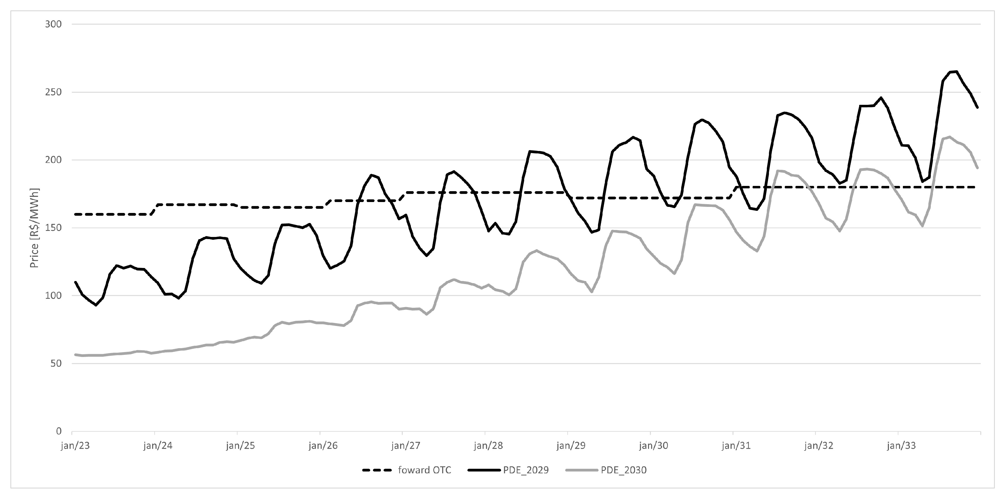
Figure 2 shows the average behavior of the prices over time in each scenario, as well as the adopted over-the-counter (OTC) price definition. The OTC forward price will represent the price profile that agents are willing to negotiate in the free market over the horizon.

The existing mix of assets for the power producer examined in this study can be seen in

Table 5. Portfolio composition.

Type	Total Physical Guarantee [MWm]	Average Cost of Operation and Maintenance [R$/MWh]	Concession Expiration
Hydraulic power plants—Group 1	38.3	0.54	31 May 2028
Hydraulic power plants—Group 2	36.0	0.54	31 July 2032
Hydraulic power plants—Group 3	128.6	0.54	31 December 2035
Hydraulic power plants—Group 4	122.8	0.54	25 August 2036
Wind power plants	67.5	0.21	31 December 2033
Sales contracts 1	−325.0	225.00	31 December 2033
Sales contracts 2	−23.0	230.00	31 December 2033

. This table compiles the company’s resources (where physical guarantee $\ge 0$) and requirements (where physical guarantee $\le 0$), categorizing them by their source type.

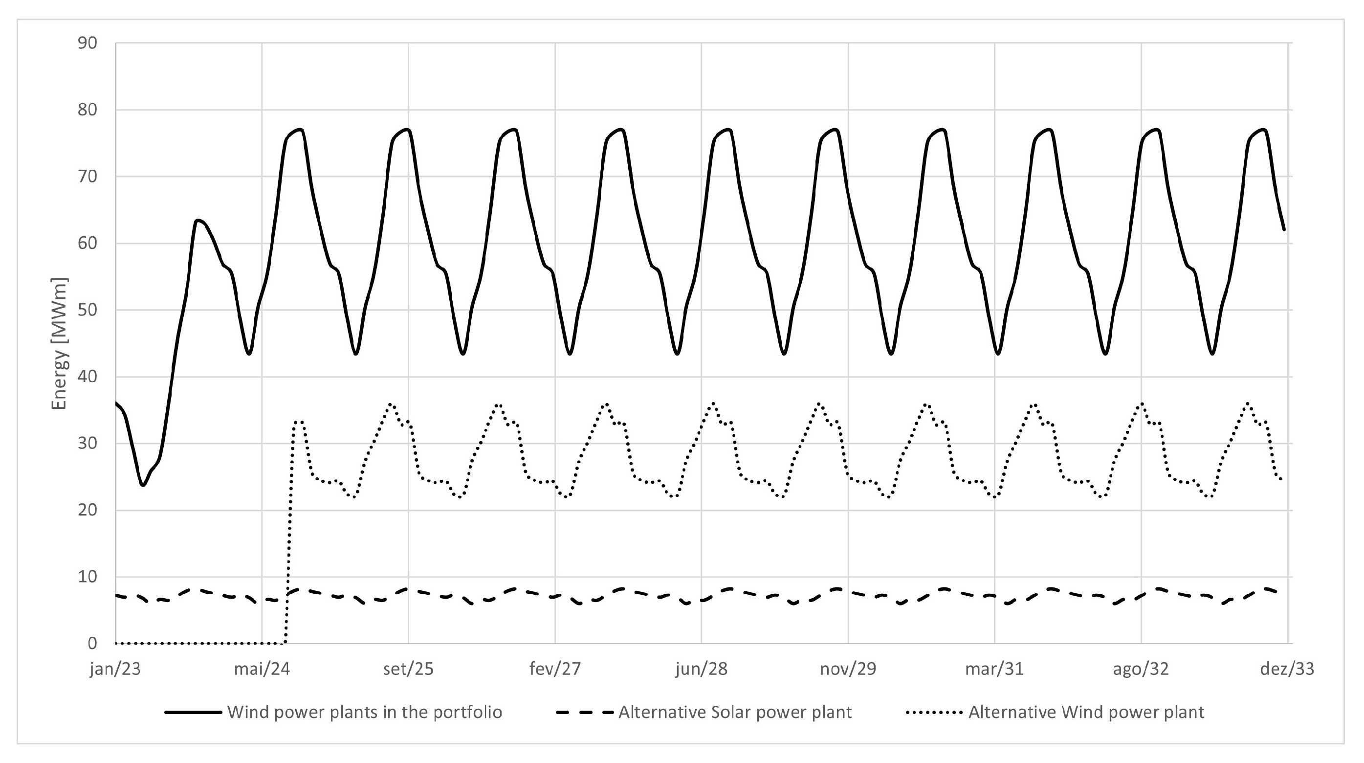
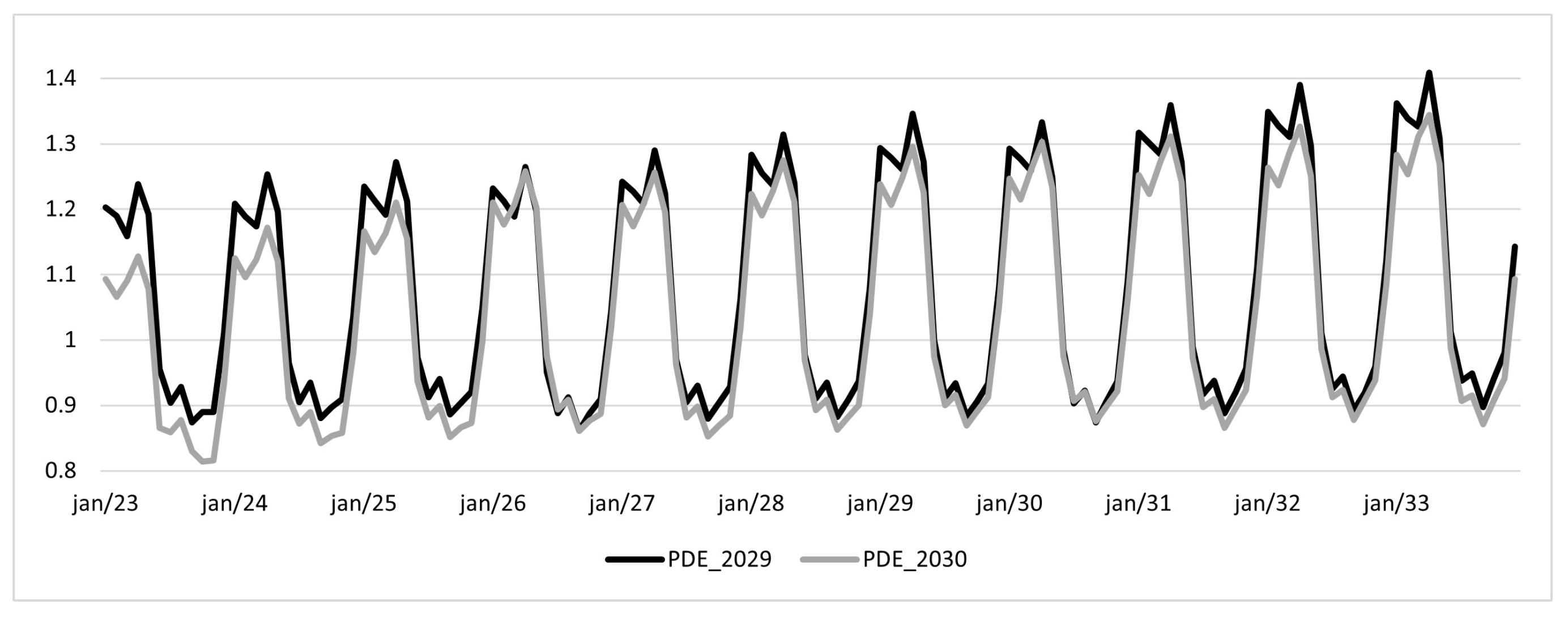
The resource considered for the plants depends on their associated generation profile, as shown in Figure 3. The hydroelectric plants in the portfolio depend on the evaluated scenario since their resource is characterized by the GSF projection for the future (shown in Figure 4), as they belong to the MRE.

The investment alternatives are described in

Table 6. Description of alternatives.

Alternative Type	Physical Guarantee (MWm)	Operation Cost (R$/MWh)	Portfolio Entry	Concession Expiration
Wind power plant	28.0	0.00	1 September 2024	31 May 2057
Solar power plant	8.0	0.00	1 January 2022	31 December 2033
Wind power plant sales contract	−28.0	210.00	1 January 2022	31 December 2033
Solar power plant sales contract	−8.0	197.50	1 September 2024	31 December 2033

, and the characteristics of the plants in question are given in

Table 7. Characteristics of the alternatives.

Name	Installed Capacity (MW)	Capacity Factor	Investment Cost (M R$)
Wind power plant	53.7	0.52	250.00
Solar power plant	47.0	0.17	172.00

. Therefore, these alternatives will be evaluated considering either the individual purchase of each plant combined with the total or partial energy sale, or the acquisition of the plants together for forming the portfolio composition. In all contracting cases, only firm contracts are considered, which are contracts with fixed volume and price over the contracting horizon, without any flexibility or premium.

The final alternatives for decision making are defined as follows:

• $X_0$: Maintain the current portfolio;
• $X_1$: Current portfolio with the addition of the solar plant with a contract sale of 100% of its physical guarantee;
• $X_2$: Current portfolio with the addition of the wind plant with a contract sale of 100% of its physical guarantee;
• $X_3$: Current portfolio with the addition of the wind plant with a contract sale of 80% of its physical guarantee;
• $X_4$: Current portfolio with the addition of the wind plant with a contract sale of 50% of its physical guarantee;
• $X_5$: Current portfolio with the addition of the wind and solar plants with a contract sale of 100% of their physical guarantees;
• $X_6$: Current portfolio with the addition of the solar plant with a contract sale of 75% of its physical guarantee;
• $X_7$: Current portfolio with the addition of the solar plant with a contract sale of 75% of its physical guarantee and the wind plant with a contract sale of 80% of its physical guarantee.

All alternatives are simulated to obtain their performance in each objective for each of the scenarios. The NPV is calculated considering an annual discount rate of 8%.

5. Results

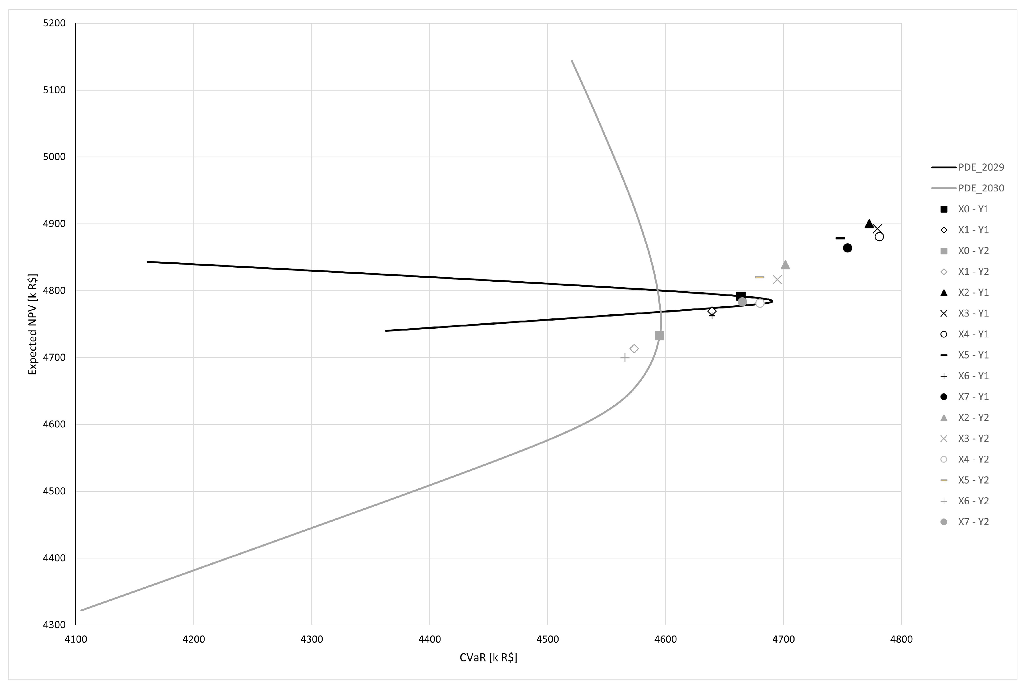
The portfolio’s behavior, as depicted in Figure 5, showcases the relationship between revenue variation and the CVaR for each scenario. Additionally, the risk associated with revenue is presented in Figure 6. The construction of the market line is carried out by manipulating the contract volume in the portfolio along a contracting range from −100 MWm to 100 MWm, where $PDE\_2029$ is transcribed as $Y_1$ and $PDE\_2030$, as $Y_2$. This calculation is carried out considering that the trading will be carried out according to the over-the-counter price (Figure 2). The market line is not considered in the decision-making process; however, it can indicate a comparison basis that can be used to invalidate some choices.

Evaluating the portfolio’s behavior in the scenarios shown in Figure 5, we notice that the portfolio’s $CVaR$ value is more responsive in the scenario with higher prices. In this scenario, options $X_2$, $X_3$, and $X_4$ outperform all other alternatives. These choices symbolize the purchase of the wind plant with different committed sales volumes in contracts. However, options that solely involve purchasing the solar plant, such as $X_1$ and $X_6$, are outperformed by the current position and should consequently be excluded from the consideration. Yet, if the solar plant is purchased along with the wind plant, as in $X_5$ or $X_7$, they outperform the current position.

The options that include the standalone purchase of solar plants continue to perform poorly in scenario $Y_2$. They are outperformed by the current position and fall within this scenario’s market curve. The standout options in this scenario are those where a substantial portion of energy from the purchased plants is committed, such as $X_2$, $X_3$, and $X_5$. Among these, option $X_2$ outperforms all others in this scenario.

Similarly, in both scenarios in Figure 6, the alternatives that stood out the most were those that consisted of the acquisition of the wind plant or simultaneously with the solar plant with the partial sale of their energy. For this figure, the total sale of the solar plant’s energy is dominated by the current position in both scenarios, and $X_5$ is also dominated by other alternatives.

To evaluate the robustness of the alternatives in the considered scenarios, payoff matrices were constructed for the objectives in question. These matrices can be seen in

Table 8. Payoff matrix of expected NPV.

Alternative	PDE_2029	PDE_2030
$X_0$	4791.51	4732.74
$X_1$	4769.46	4713.26
$X_2$	4900.36	4839.31
$X_3$	4892.69	4816.45
$X_4$	4880.84	4781.12
$X_5$	4878.31	4819.83
$X_6$	4762.62	4699.49
$X_7$	4863.80	4783.20

,

Table 9. Payoff matrix of CVaR.

Alternative	PDE_2029	PDE_2030
$X_0$	4664.09	4594.92
$X_1$	4639.48	4573.23
$X_2$	4772.78	4701.65
$X_3$	4779.64	4694.74
$X_4$	4781.34	4680.04
$X_5$	4748.16	4679.91
$X_6$	4639.42	4565.59
$X_7$	4754.29	4665.14

,

Table 10. Matriz payoff of RaR.

Alternative	PDE_2029	PDE_2030
$X_0$	127.42	137.82
$X_1$	129.98	140.03
$X_2$	127.58	137.66
$X_3$	113.05	121.71
$X_4$	99.50	101.08
$X_5$	130.14	139.92
$X_6$	123.20	133.90
$X_7$	109.50	118.06

and

Table 11. Payoff matrix of InS.

Alternative	PDE_2029	PDE_2030
$X_0$	0.00	0.00
$X_1$	143.45	143.45
$X_2$	119.91	119.91
$X_3$	111.46	111.46
$X_4$	94.05	94.05
$X_5$	125.14	125.14
$X_6$	133.94	133.94
$X_7$	116.34	116.34

.

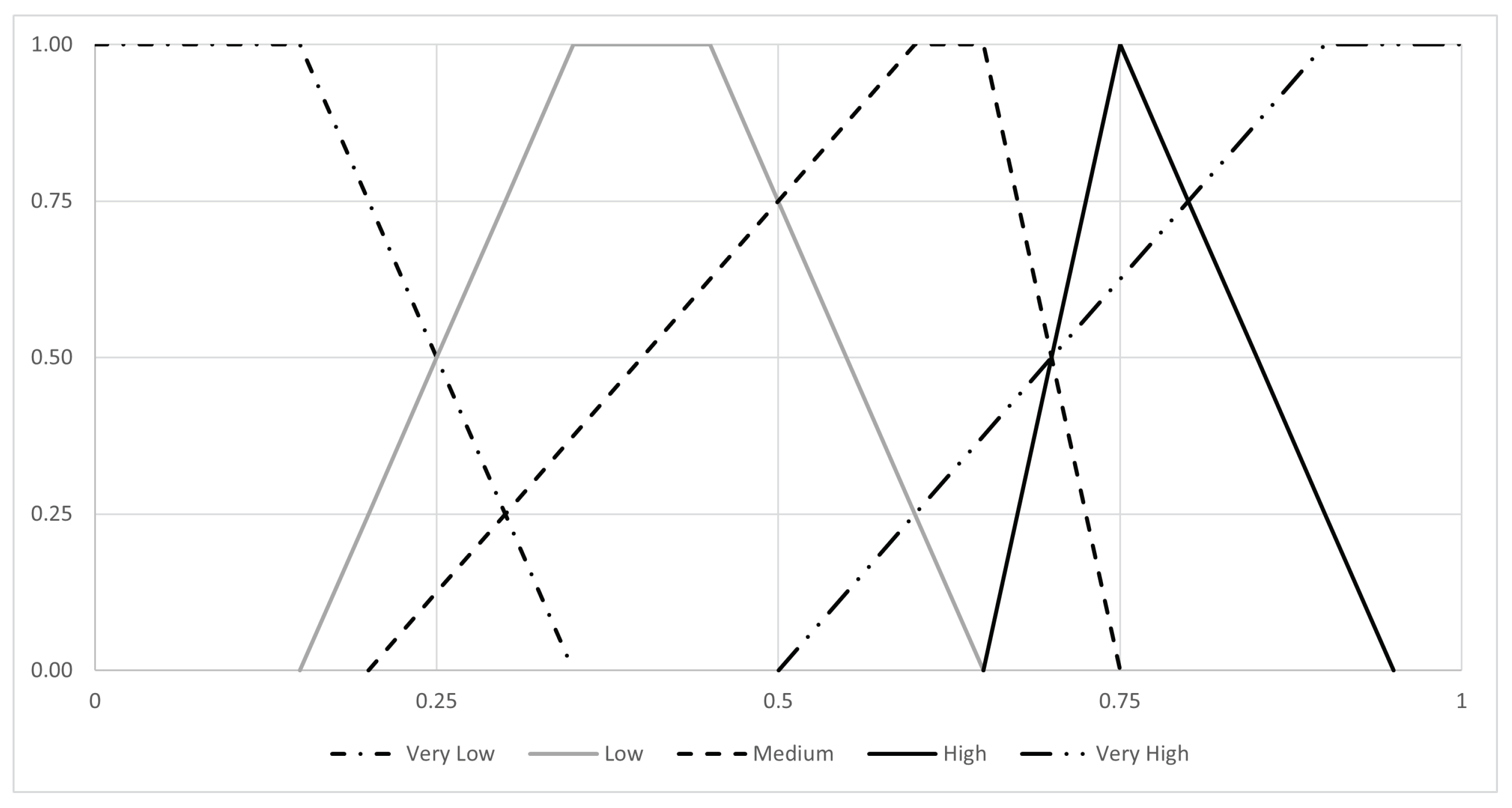
The results presented in

Table 12. $\langle X,F\rangle$ model result.

Alternative	Wald	Laplace	Savage	Hurwicz
$X_0$	0.00	0.00	0.00	0.00
$X_1$	0.00	0.00	0.00	0.00
$X_2$	0.06	0.07	0.06	0.06
$X_3$	0.47	0.51	0.47	0.49
$X_4$	0.58	0.66	0.58	0.65
$X_5$	0.00	0.00	0.00	0.00
$X_6$	0.00	0.00	0.00	0.00
$X_7$	0.56	0.61	0.56	0.59

can be considered as the final response to the analysis of the $〈X,F〉$ models. According to the results in this table, alternatives $X_0$, $X_1$, $X_2$, $X_5$, and $X_6$ are to be discarded from the decision-making process. On the other hand, alternative $X_3$ received an intermediate score in all the selection criteria. Meanwhile, it is not possible to define a significant relevance between alternatives $X_4$ and $X_7$, making it necessary to evaluate these two alternatives using additional criteria. Decision makers assessed these two alternatives according to the two additional criteria using fuzzy estimates presented in Figure 7, where the vertical axis represents $\mu \left(X_k\right)$ [13].

For the criterion of prioritizing alternatives that have greater synergy with the portfolio’s resources, the following were indicated: $X_4—\mathrm{high}$; $X_7—\mathrm{very}\mathrm{high}$. As for the criterion of prioritizing alternatives with the lowest operational risk, the following estimates were indicated: $X_4—\mathrm{medium}$; $X_7—\mathrm{high}$. Using (26) and (27) for these estimates it is possible to contruct the following non-reciprocal fuzzy preference relation as:

$$\begin{array}{cc}{R}_1=\left[\begin{array}{cc}1& 0.75\\ 1& 1\end{array}\right],& R_2=\left[\begin{array}{cc}1& 0.5\\ 1& 1\end{array}\right],\end{array}$$

(36)

where $R_1$ is the preference relation matrix concerning prioritizing alternatives that have the greatest synergy with the portfolio’s resources, and $R_2$ relates to prioritizing alternatives with the lowest operational risk.

Considering that the criteria have the same importance and since the evaluations of the alternatives resulted in a convergence of preference for $X_7$, the non-strict fuzzy preference relation matrix for the development of the $〈X,F〉$ model is equal to $R_2$. Therefore, one can obtain the membership function of the strict fuzzy preference relation as follows:

$$P=\left[\begin{array}{cc}0& 0\\ 0.5& 0\end{array}\right],$$

(37)

and finally, the use of Equation (31) allows us to obtain the following membership function of the fuzzy set of non-dominated alternatives:

$$ND=\left[\begin{array}{cc}0.5& 1\end{array}\right],$$

(38)

that justifies the choice of $X_7$.

6. Conclusions

The present work reflects research results related to applying the techniques of multicriteria decision making under conditions of uncertainty to long-term investment planning in the electricity sector. By analyzing the energy portfolio of the company based on the proposed approach, it is possible to quantify the expected revenue and the financial risks involved in acquiring energy assets. The measurement of portfolio revenue from investment options utilizes the expected $NPV$ across different scenarios, with risk quantified using the $CVaR$. An evaluation of the portfolio’s revenue at risk is also conducted. To improve the investment analysis, three further objectives have been introduced, two of which possess a qualitative nature.

In the given illustrative example, evaluations of investments in alternatives potentially impacting the portfolio’s performance over time are conducted. The selection of an alternative impacts the energy balance of the agent, modifying exposure in the long-term scenarios under assessment. This, in turn, influences the values of the objective functions. It is observed that the outcomes display sensitivity to the PLD and GSF projections sourced from NEWAVE. A robust solution in the application example involves the incorporation of both solar and wind plants into the existing portfolio, without committing all energy from these plants to contract sales, thus retaining a percentage exposed to the spot price.

Employment of the proposed methodology facilitates the evaluation of alternatives beyond their associated costs, considering factors pertinent to the agent such as the insurance index (InS), synergy with the resources in the portfolio, and operational risks. Utilizing multiple scenarios enables the simultaneous consideration of different specific situations, constituting a significant step forward in addressing issues associated with using NEWAVE as input for the long-term decision model. The use of the objectives of the qualitative character allows for the distinction and selection of non-dominated alternatives previously evaluated within the $\langle X,F\rangle$ decision models. Although, in this work, the approach to constructing robust (non-dominated) solutions in multicriteria (multiobjective) decision making under conditions of uncertainty was applied to the problem of energy portfolio management, it is of a universal character and can be applied to solving wide classes of problems related to decision making in conditions of uncertainty. However, it is recognized that future work would benefit from considering additional scenarios derived from different information sources.

References

1. Božić, Z.; Dobromirov, D.; Arsić, J.; Radišić, M.; Ślusarczyk, B. Power Exchange Prices: Comparison of Volatility in European Markets. Energies 2020, 13, 5620. [Google Scholar] [CrossRef]
2. Sadeghi, M.; Shavvalpour, S. Energy risk management and value at risk modeling. Energy Policy 2006, 34, 3367–3373. [Google Scholar] [CrossRef]
3. Weron, R. Energy price risk management. Phys. A Stat. Mech. Its Appl. 2000, 285, 127–134. [Google Scholar] [CrossRef]
4. Chawda, S.; Bhakar, R.; Mathuria, P. Uncertainty and risk management in electricity market: Challenges and opportunities. In Proceedings of the 2016 National Power Systems Conference (NPSC), Bhubaneswar, India, 19–21 December 2016; pp. 1–6. [Google Scholar] [CrossRef]
5. Dahlgren, R.; Liu, C.C.; Lawarree, J. Risk assessment in energy trading. IEEE Trans. Power Syst. 2003, 18, 503–511. [Google Scholar] [CrossRef]
6. Denton, M.; Palmer, A.; Masiello, R.; Skantze, P. Managing market risk in energy. IEEE Trans. Power Syst. 2003, 18, 494–502. [Google Scholar] [CrossRef]
7. Pérez Odeh, R.; Watts, D.; Negrete-Pincetic, M. Portfolio applications in electricity markets review: Private investor and manager perspective trends. Renew. Sustain. Energy Rev. 2018, 81, 192–204. [Google Scholar] [CrossRef]
8. Fu, Y.; Sun, Q.; Wennersten, R. Effectiveness of the CVaR method in risk management in an integrated energy system. Energy Rep. 2020, 6, 1010–1015. [Google Scholar] [CrossRef]
9. Peixoto, G.M.; Pereira, R.B.; da Silva Amorim, L.; Machado-Coelho, T.M.; Soares, G.L.; Parma, G.G. Analysis of the Participation of Small Hydroelectric Power Plants in the Energy Reallocation Mechanism (in portuguese). In Proceedings of the 14º Simpósio Brasileiro de Automação Inteligente, Ouro Preto, Brazil, 27–30 October 2019; pp. 1–7. [Google Scholar] [CrossRef]
10. Gökgöz, F.; Atmaca, M.E. Portfolio optimization under lower partial moments in emerging electricity markets: Evidence from Turkey. Renew. Sustain. Energy Rev. 2017, 67, 437–449. [Google Scholar] [CrossRef]
11. Ekel, P.; Pedrycz, W.; Pereira, J. Multicriteria Decision-Making under Conditions of Uncertainty: A Fuzzy Set Perspective; John Wiley & Sons: Hoboken, NJ, USA, 2020. [Google Scholar]
12. Maceiral, M.; Penna, D.; Diniz, A.; Pinto, R.; Melo, A.; Vasconcellos, C.; Cruz, C. Twenty Years of Application of Stochastic Dual Dynamic Programming in Official and Agent Studies in Brazil-Main Features and Improvements on the NEWAVE Model. In Proceedings of the 2018 Power Systems Computation Conference (PSCC), Dublin, Ireland, 11–15 June 2018; pp. 1–7. [Google Scholar] [CrossRef]
13. Ramalho, F.D.; Ekel, P.Y.; Pedrycz, W.; Pereira Júnior, J.G.; Soares, G.L. Multicriteria decision making under conditions of uncertainty in application to multiobjective allocation of resources. Inf. Fusion 2019, 49, 249–261. [Google Scholar] [CrossRef]
14. Abba, Z.; Balta-Ozkan, N.; Hart, P. A holistic risk management framework for renewable energy investments. Renew. Sustain. Energy Rev. 2022, 160, 112305. [Google Scholar] [CrossRef]
15. Camargo, L.A.S.; Leonel, L.D.; Rosa, P.S.; Ramos, D.S. Optimal Portfolio Selection of Wind Power Plants Using a Stochastic Risk-Averse Optimization Model, Considering the Wind Complementarity of the Sites and a Budget Constraint. Energy Power Eng. 2020, 12, 459–476. [Google Scholar] [CrossRef]
16. Bradshaw, A. Regulatory change and innovation in Latin America: The case of renewable energy in Brazil. Util. Policy 2017, 49, 156–164. [Google Scholar] [CrossRef]
17. Ilbahar, E.; Kahraman, C.; Cebi, S. Risk assessment of renewable energy investments: A modified failure mode and effect analysis based on prospect theory and intuitionistic fuzzy AHP. Energy 2022, 239, 1–11. [Google Scholar] [CrossRef]
18. Martínez, L.; Dinçer, H.; Yüksel, S. A hybrid decision making approach for new service development process of renewable energy investment. Appl. Soft Comput. 2023, 133, 1–17. [Google Scholar] [CrossRef]
19. de Freitas, R.A.; Vogel, E.P.; Korzenowski, A.L.; Oliveira Rocha, L.A. Stochastic model to aid decision making on investments in renewable energy generation: Portfolio diffusion and investor risk aversion. Renew. Energy 2020, 162, 1161–1176. [Google Scholar] [CrossRef]
20. Yang, L.; Sun, Q.; Zhang, N.; Li, Y. Indirect Multi-Energy Transactions of Energy Internet with Deep Reinforcement Learning Approach. IEEE Trans. Power Syst. 2022, 37, 4067–4077. [Google Scholar] [CrossRef]
21. Wang, L.; Zhou, Q.; Xiong, Z.; Zhu, Z.; Jiang, C.; Xu, R.; Li, Z. Security constrained decentralized peer-to-peer transactive energy trading in distribution systems. CSEE J. Power Energy Syst. 2022, 8, 188–197. [Google Scholar] [CrossRef]
22. Pedrycz, W.; Ekel, P.; Parreiras, R. Fuzzy Multicriteria Decision-Making: Models, Methods and Applications; John Wiley & Sons: Hoboken, NJ, USA, 2011. [Google Scholar]
23. Santos, F.F.G.D.; Vieira, D.A.G.; Saldanha, R.R.; Lisboa, A.C.; de Castro Lobato, M.V. Seasonal energy trading portfolio based on multiobjective optimisation. Int. J. Logist. Syst. Manag. 2014, 17, 180. [Google Scholar] [CrossRef]
24. Luce, R.; Raiffa, H. Games and Decisions; John Wiley & Sons: Hoboken, NJ, USA, 1957. [Google Scholar]
25. Raiffa, H. Decision Analysis: Introductory Lectures on Choices under Uncertainty; Addison-Wesley: Boston, MA, USA, 1968. [Google Scholar]
26. Belyaev, L.S. A Practical Approach to Choosing Alternative Solutions to Complex Optimization Problems under Uncertainty. Int. Inst. Appl. Syst. Anal. 1977, 1, 1–60. [Google Scholar]
27. Hodges, J.L.; Lehmann, E.L. The use of Previous Experience in Reaching Statistical Decisions. Ann. Math. Stat. 1952, 23, 396–407. [Google Scholar] [CrossRef]
28. Trukhaev, R. Models of Decision Making in Conditions of Uncertainty; Nauka: Moscow, Russia, 1981. [Google Scholar]
29. Figueiredo, L.R.; Frej, E.A.; Soares, G.L.; Ekel, P.Y. Group Decision-Based Construction of Scenarios for Multicriteria Analysis in Conditions of Uncertainty on the Basis of Quantitative and Qualitative Information. Group Decis. Negot. 2021, 30, 665–696. [Google Scholar] [CrossRef]
30. Ekel, P. Fuzzy sets and models of decision making. Comput. Math. Appl. 2002, 44, 863–875. [Google Scholar] [CrossRef]
31. Bellman, R.E.; Zadeh, L.A. Decision-Making in a Fuzzy Environment. Manag. Sci. 1970, 17, 141–164. [Google Scholar] [CrossRef]
32. Ekel, P.; Kokshenev, I.; Parreiras, R.; Pedrycz, W.; Pereira, J., Jr. Multiobjective and multiattribute decision making in a fuzzy environment and their power engineering applications. Inf. Sci. 2016, 361-362, 100–119. [Google Scholar] [CrossRef]
33. Pereira, J.; Ekel, P.; Palhares, R.; Parreiras, R. On multicriteria decision making under conditions of uncertainty. Inf. Sci. 2015, 324, 44–59. [Google Scholar] [CrossRef]
34. Ralston, B.; Wilson, I. The Scenario Planning Handbook; South-Western: Nashville, TN, USA, 2006. [Google Scholar]
35. Amer, M.; Daim, T.U.; Jetter, A. A review of scenario planning. Futures 2013, 46, 23–40. [Google Scholar] [CrossRef]
36. Ekel, P.; Martins, C.; Pereira, J.; Palhares, R.; Canha, L. Fuzzy set based multiobjective allocation of resources and its applications. Comput. Math. Appl. 2006, 52, 197–210. [Google Scholar] [CrossRef]
37. Yager, R. On ordered weighted averaging aggregation operators in multicriteria decisionmaking. IEEE Trans. Syst. Man Cybern. 1988, 18, 183–190. [Google Scholar] [CrossRef]
38. Pinheiro Neto, D.; Domingues, E.G.; Coimbra, A.P.; de Almeida, A.T.; Alves, A.J.; Calixto, W.P. Portfolio optimization of renewable energy assets: Hydro, wind, and photovoltaic energy in the regulated market in Brazil. Energy Econ. 2017, 64, 238–250. [Google Scholar] [CrossRef]
39. Rockafellar, R.T.; Uryasev, S. Optimization of conditional value-at-risk. J. Risk 2000, 2, 21–41. [Google Scholar] [CrossRef]
40. Carrano, E.G.; Tarôco, C.G.; Neto, O.M.; Takahashi, R.H. A multiobjective hybrid evolutionary algorithm for robust design of distribution networks. Int. J. Electr. Power Energy Syst. 2014, 63, 645–656. [Google Scholar] [CrossRef]
41. Empresa de Pesquisa Energética. Plano Decenal de Expansão de Energia 2029; Ministério de Minas e Energia: Lisboa, Portugal, 2020. [Google Scholar]
42. Empresa de Pesquisa Energética. Plano Decenal de Expansão de Energia 2030; Ministério de Minas e Energia: Lisboa, Portugal, 2021. [Google Scholar]
Figure 1. Revenue distribution estimates.
Energies 16 06089 g001
Figure 2. Average PLD of scenarios and forward over-the-counter price.
Energies 16 06089 g002
Figure 3. Predicted generation profile of the plants.
Energies 16 06089 g003
Figure 4. Average GSF in the scenarios.
Energies 16 06089 g004
Figure 5. NPV vs. CVaR.
Energies 16 06089 g005
Figure 6. NPV vs. RaR.
Energies 16 06089 g006
Figure 7. Qualitative scales based on fuzzy sets used for objectives based on qualitative information. Source: [13].
Energies 16 06089 g007