Research on Load Forecasting of Novel Power System Based on Efficient Federated Transfer Learning

Abstract

The load forecasting research for an NPS faces challenges including a high model accuracy, non-sharing of data, and a high communication cost. This paper proposes a load forecasting method for an NPS, based on efficient federated transfer learning (FTL). The adversarial feature extractor is added on the basis that FTL can effectively transfer the parameter features of the non-mask load to the local load data, and make up for the loss of mask load prediction accuracy. In order to improve the efficiency of the gradient compression of federated learning (FL), a depth dynamic threshold compression sensing method is proposed, which replaces the sparse signal in compressed sensing via the U-Net model and achieves an observation dimension reduction through a convolutional neural network (CNN). The experimental results show that the mean absolute percentage error (MAPE) and the root-mean-square error (RMSE) of the load forecasting method proposed in this paper are reduced by 9.6% and 2.31 kW, on average, when the load data are covered up to different degrees. Compared with the traditional FL model, the proposed compression algorithm saves 23.5% of the communication cost, without changing the accuracy of the model. The proposed prediction framework is easily interpretable, and robust under different validation metrics.

1. Introduction

The goal of a novel power system (NPS) is to achieve a sustainable, efficient, and secure energy supply. Accurate short-term load forecasting is one of the key technologies to ensure the safe and stable operation of an NPS. However, the traditional forecasting method faces difficulties, such as large number of users, a high load heterogeneity, a high volatility, and a high randomness, meaning that it is difficult to meet the requirements of load forecasting in an NPS [1,2,3].

With the continuous deepening of distributed power generation technology, photovoltaic, wind, and other types of new energy power generation equipment are widely installed in user terminals, but with the limits of the privacy of user data, it is impossible to concentrate the load data to train forecasting models [4,5]. Moreover, the load data are usually processed by multiple masks, and the reverse decoding process also involves the permissions of sensitive information. Therefore, the unprocessed mask load will greatly reduce the final accuracy of the prediction model [6].

The proposal of federated learning breaks through the regional limitation of data privacy, and allows clients to train global models without sharing data, but frequent cloud-edge communication will generate a large communication load in the process of gradient transmission, and the communication overhead will become larger and larger, as the number of clients increases.

Therefore, the research into load forecasting under the background of an NPS faces the complexity and uncertainty of the distributed power supply, on the one hand. On the other hand, the continuous information and intelligence of the power industry provides a large amount of power load data for the communication system of the smart grid, and also increases the training cost of the forecasting model.

To summarize, this paper studies NPS load forecasting, based on efficient FTL. The innovations are as follows:

• An adversarial predictive model training method based on transfer federation learning is proposed. This method extracts the common feature vector between the global model and the local data through adversarial training, so as to compensate the loss of mask load in the prediction accuracy, and improve the prediction accuracy.
• In order to improve the efficiency of the gradient compression in federated learning (FL), a compressed sensing method based on the depth dynamic threshold is proposed, which combines compressed sensing with deep learning. This method replaces the sparse signal in compressed sensing with a U-Net model, and achieves an observation dimension reduction through a convolutional neural network (CNN).

2. Related Works

2.1. Research on Load Forecasting under Data Privacy

At present, power load forecasting methods are mainly divided into two kinds: a statistical theory based on a time series method, and an intelligent algorithm based on an artificial neural network (ANN) [7]. The traditional time series method can collect historical load data and build a mathematical model to forecast the load, but this method is very dependent on the load data, and cannot deal with the influence of non-human factors well. The learning ability of ANN means that it can be quickly applied in the field of load forecasting. The literature [8,9] combines the fuzzy reasoning method, gray model, and ANN for load forecasting, respectively. In the literature [10], a neural network forecasting model combining the grey model and Elman network was used to forecast the load. The literature [11] combines wavelet analysis and a neural network to make a load prediction with a higher accuracy. However, due to the wide application and grid connection of a large number of intelligent acquisition terminals, such as wireless sensor networks, it is difficult to solve the problem of data privacy in the load forecasting of an NPS.

Federated learning is a distributed machine learning framework, in which multiple parties (such as devices or institutions) work together to train a shared global model, without having to centralize their raw datasets to a single central server. The application of federated learning to the load forecasting of NPSs can, at the same time, protect the data privacy of all participants, and train the forecasting model [12]. However, the mask load is usually used in the data preprocessing stage of load prediction. When the load data are missing or unavailable, the data are populated by a specific value (such as 0 or NaN), which ensures the integrity of the user’s load data. In each round of federated learning training, the global model needs to be updated with local data, and the masked load data will dilute the feature distribution of the global model, increase the number of federated learning communication rounds, and affect the accuracy of the prediction model.

Federated transfer learning aims to improve the model performance and generalization, by leveraging shared model knowledge among participants, to transfer knowledge learned via one or more participants to other participants. Wang et al. [13] proposed domain adaptive federated transfer learning to realize the high-precision diagnosis of insulation defects in a gas-insulated switchgear. Cheng et al. [14] combined the customer choice scheme of federal transfer learning and reinforcement learning, to achieve the highest intrusion detection accuracy within budget constraints. In the framework of federated learning, the transfer learning method can transfer the data features of the non-mask load to the local model directly, using the global model as the source domain, without additional mask load filling processing.

2.2. Efficient Communication Federation Learning

A key challenge in federated learning is communication overhead. On the one hand, in federated learning, the participating client devices can usually only allocate a small amount of communication resources to federated learning; on the other hand, advanced machine learning applications deployed on edge devices increasingly use complex deep neural networks (DNNS). Gradient compression is necessary for use in resource-constrained environments. To solve the problem of the high communication cost of federated learning, researchers have proposed many gradient compression mechanisms. At present, there are three main methods: sparse, quantization, and compressed sensing [15,16,17].

There are many sparse gradient compression methods. Yin et al. [18] proposed that only gradients greater than a certain threshold should be transmitted to the server, to reduce traffic. Chen et al. [19] proposed an alternative method, of sorting the gradients, and then transmitting only the first P% of the gradients to the server, and storing the rest in the residual vector. Quantization-based gradient compression can compress the amount of traffic that is uploaded and sent in the federated learning framework. In the 1-bit quantization proposed by Ren et al. [20], the client only needs to upload the symbol of the local model gradient to the server.

Compared to traditional compression, compressed sensing (CS) can recover a signal with a sampling frequency much lower than that required by the classical Nyquist sampling theorem. The general idea is to project a sparse or compressible high-dimensional signal into a low-dimensional space, with a measurement matrix satisfying certain conditions, and then to restore the signal with high probability, by solving an optimization problem [21]. Because of these advantages, compressed sensing is widely used in signal processing, but is hardly used in federated learning. To the best of the author’s knowledge, Li et al. [22] recently applied compressed sensing to federated learning, and showed a good performance in terms of communication efficiency and model accuracy. However, each round of training for the algorithm by Li et al. consists of two stages, both of which require the client to interact with the server, resulting in additional communication burdens. Bora et al. proposed to replace compressed sensing using generative models (CSGM) [23], to achieve image reconstruction, but the model is complex and slowly trained. Google Deep Mind proposed a deep compressed sensing model (Deep CS) [24], which has a better reconstruction quality and a faster speed than the CSGM. In this paper, a compressed sensing method based on a depth dynamic threshold is proposed, which reduces the communication overhead of uploading and underweight data in the federated learning framework, and is superior to the existing gradient compression algorithm in convergence speed and accuracy.

3. Adversarial Transfer Federation Algorithm Framework for Efficient Communication

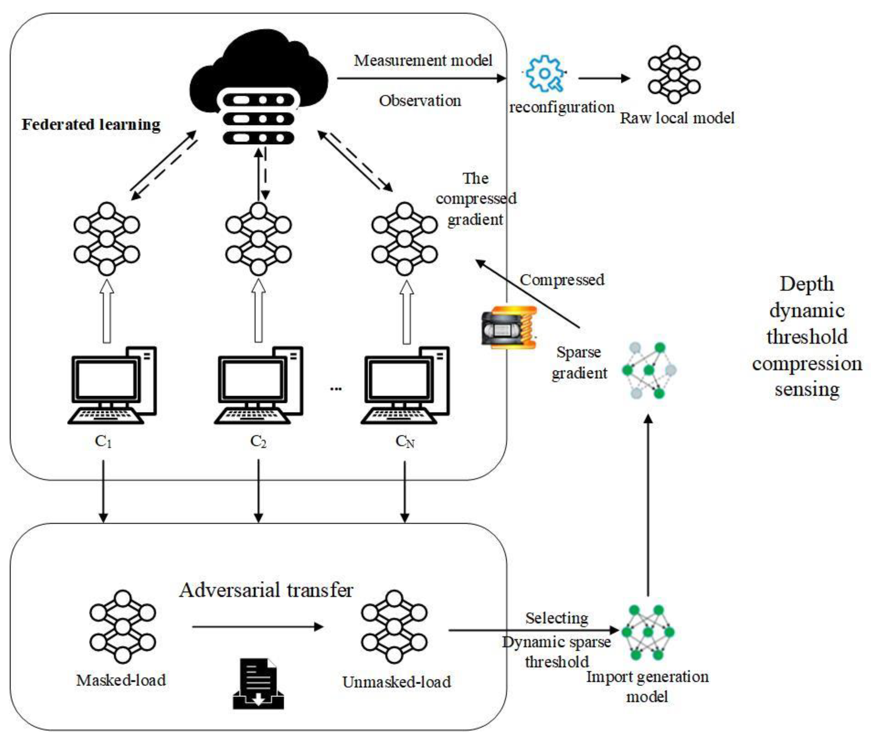
Based on the difficulties of load forecasting in NPSs, this paper proposes a scheme of load forecasting, based on efficient communication, for federated transfer learning. Firstly, federated transfer learning is used to solve the data privacy problem between different grid regions, and to improve the influence of the mask load on the accuracy of the prediction model. Secondly, according to signal sparsity and the added attention mechanism, a compressed sensing method based on a depth dynamic threshold is proposed, which effectively reduces the huge overhead caused by the frequent cloud-edge communication in federated learning. The specific process framework of the scheme is shown in Figure 1.

It is assumed that the participants under the federated learning framework belong to different power grid parks, and the user load data are not interoperable. After the federated learning training starts, the cloud service center, firstly, delivers the trained global model parameters, and the client locally migrates the characteristic parameters of the non-mask load to the mask load, and completes the local model update. Secondly, a U-Net structure is used to generate the model, to realize the signal sparse process, and the model gradient features that need to be uploaded to the cloud server are sparse. Finally, the cloud server reconstructs the signal, aggregates all the models, and generates the global model for the next round of federated learning.

3.1. Adversarial Federated Transfer Learning

Aiming at the mask load problem in the load forecasting of NPSs, this paper proposes an adversarial federated transfer learning system, the specific framework of which is shown in Figure 2. The training framework consists of three modules; namely, feature extraction, result prediction, and adversarial training.

In the federated transfer learning system proposed in this paper, the mask load is taken as the target domain $D_T={\left\{\left(x_T^i\right)\right\}}_{i=1}^{n_T}$; the unmasked load in the global model parameter serves as the source domain $D_S={\left\{\left(x_S^i,y_S^i\right)\right\}}_{i=1}^{n_S}$. Where n_T and n_S are the amount of sample data in n_S and n_S, $x_S^i$ represents the global model unmasked load data input the previous time, during the i round of training. $y_S^i$ represents the future time. Different from traditional transfer learning, the adversarial federated transfer learning proposed in this paper requires the adversarial transfer of two different load data, so the number of n_S is not much larger than n_T, but similar. Based on the above related theories, the proposed method trains the prediction model of D_T through adversarial training, and transfers knowledge from D_S to improve the prediction accuracy. The specific training process is as follows:

• First, input global model parameter X_S and client local data X_T (mask load). The two input data are processed by the feature extractor G_f and the feature vectors are extracted as f_S and f_T.
• The result predictor G_o receives the feature vector f_S and updates the predicted loss L_o.
• The adversarial trainer G_d divides the features into D_T and D_S, uses gradient reverse layer (GRL) for adversarial training, and updates L_d to minimize the adversarial loss.
• Output load data, complete the local FL.

Steps 2 and 3 can be performed simultaneously offline, until the next round of FL local training begins. In the process of forward propagation, the input data are first processed using the feature processor G_f, with the initialization parameter θ_f, and then the result predictor G_y predicts the load, and calculates the predicted loss L_o based on the mean square error:

$$L_o\left(y_S,o_S\right)=\frac{1}{n}{{\displaystyle \sum _{i=1}^{n_i}\left(y_S^i-o_S^i\right)}}^2$$

(1)

where n_S is the total number of output samples in D_S. Against the trainer G_d classification feature vector, GRL is used to maintain the calculation results of forward propagation, but the polarity of the gradient calculation is changed during the late update period. The calculation of counterloss L_d based on the binary cross entropy error is:

$$L_d\left(d_S,d_T\right)=-\left(\frac{1}{n_S}{\displaystyle \sum _{i=1}^{n_S}\ln \left(d_S^i\right)+\frac{1}{n_T}{\displaystyle \sum _{i=1}^{n_T}\ln \left(1-d_T^i\right)}}\right)$$

(2)

$d_S^i$ and $d_{\mathrm{T}}^i$ represent the probability of the I-th eigenvector of D_S and D_T, respectively. If d = 1, the eigenvector comes from D_S; otherwise, if d = 0, the eigenvector comes from D_T.

Gradient descent is adopted in the training of backward propagation. In the process of backward propagation, the result predictor and adversarial trainer also update the parameters to minimize L_y and L_o, as shown in Formulas (3) and (4):

$${\theta }_{o+1}={\theta }_o-{\lambda }_o\frac{\partial L_o\left(y_S,o_S\right)}{\partial {\theta }_o}$$

(3)

$${\theta }_{d+1}={\theta }_d-{\lambda }_d\frac{\partial L_d\left(d_S,d_T\right)}{\partial {\theta }_d}$$

(4)

where θ_o and θ_d represent the parameters in the result predictor and adversarial trainer models, respectively.

After the forward and backward propagation is completed, the output data are finally combined in the feature extractor. The cost function of the feature extractor L_f can be expressed by Formula (5):

$$L_f=L_o\left(y_S,o_S\right)+L_{div}\left(f_S,f_T\right)$$

(5)

where L_div represents the deviation between f_S and f_T, which can be represented by the following formula:

$$L_{div}\left(f_S,f_T\right)=2\left(1-2\sigma \right)$$

(6)

where σ represents the calculation error of the counter trainer, so L_f can be further expressed as Formula (7):

$$L_f=L_o\left(y_S,o_S\right)+2\left(1-L_d\left(d_S,d_T\right)\right)$$

(7)

Combining the above reasoning process, λ_f,o and λ_f,d are the learning rates of the outcome predictor and adversarial trainer, respectively. Then, the final data output can be expressed as:

$${\theta }_{f+1}={\theta }_f-{\lambda }_{f,o}\frac{\partial L_o\left(y_S,o_S\right)}{\partial {\theta }_f}+{\lambda }_{f,d}\frac{\partial L_d\left(d_S,o_T\right)}{\partial {\theta }_f}$$

(8)

The mask load feature vector, after counter training, can be very compatible with the non-mask load in the output predictor, meaning that load data with a similar feature quantity can be output, and a prediction model with a higher accuracy can be trained.

3.2. Compressed Sensing Based on Dynamic Threshold of Depth

This paper presents a depth dynamic threshold compression sensing algorithm (depth dynamic threshold compression sensing, DDTCS). The sparse process of the federated learning gradient signal based on compressed sensing is replaced by a generative model; that is, the original signal no longer needs to be sparsely processed, and the dynamic threshold of sparsity is set. Finally, the measurement matrix is replaced by a CNN, which is called the measurement model. If we let the sparse gradient be represented as x and the margin gradient be represented as n, the original signal y with sparse gradient can be represented as:

y = x + n

(9)

y is pretreated to obtain $\widehat{y}$, sparse signal $\widehat{x}$ = G_θ ($\widehat{y}$) can be generated by input generation model G_θ, and x and $\widehat{x}$ then obtain their respective observed signals through the measurement model. When the error between two observation signals is the smallest, $\widehat{x}$ is the reconstructed original signal. The generation model adopts a U-Net structure, as shown in Figure 3, which consists of four parts: the coding network, skip connection, attention mechanism, and decoding network. The coding network consists of 11 subsampling modules, in which the original gradient signal is obtained via the convolution operation, and the activation function selects PReLU. The decoding network is composed of 11 up-sampling modules, which is the inverse process of the coding network. The gradient signal with the same length of time as the input signal is recovered via deconvolution.

In order to prevent the loss of signal detail features, a jump connection is added between the coding network and the decoding network, and an attention mechanism is added to the last layer of the jump connection [6,7], to prune the gradient signal features and remove irrelevant features. The structure of the attention mechanism is shown in Figure 4.

The input of the attention mechanism is the output of the down-sampled module (V) and the output of the up-sampled module (Q) in the generation model; W_q, W_v, and W_qv represent the weight of the one-dimensional convolution; b_q, b_v, and b_qv represent the bias; W_att represents the obtained attention coefficient; after multiplication with V, the output feature graph V_att after passing the attention is obtained. The process of the signal passing through the attention mechanism can be expressed as the process of solving Equation (11), where P[·] and S{·} represent the activation functions PReLU and sigmoid, respectively:

$$V_{\mathrm{att}}=VS\left\{{\mathrm{w}}_{\mathrm{qv}}P\left[\left({\mathrm{w}}_{\mathrm{q}}Q+{\mathrm{b}}_{\mathrm{q}}\right)+\left({\mathrm{w}}_{\mathrm{v}}V+{\mathrm{b}}_{\mathrm{v}}\right)\right]+{\mathrm{b}}_{\mathrm{qv}}\right\}$$

(10)

In the process of compressed sensing, compression is actually very simple, and the focus is on the reconstruction of the signal, and the reconstruction recovery accuracy of the signal is closely related to the sparsity. When the same signal recovery accuracy is achieved, the recovery ability of a low-sparsity signal is stronger, and it is less likely to cause information loss. Therefore, a judgment can be made when the client compresses the model to compare the specific threshold data sizes of different sparse thresholds, as follows. If the threshold data under a high threshold show a small gap with the threshold data of a low threshold, it indicates that there are more contents with a large update range, and then a high threshold is used for compression. Otherwise, only a small number of data have been updated significantly, and a low threshold is used for compression.

We let the user model update amplitude be $y_{i,i}^{abs}$ and the parameter be $\alpha \in [0.7,1)$. User i locally determines the threshold ${th}_{i,t}$ for sparsity during the T-round training according to the given threshold instruction. We let the smallest value of the data with $y_{i,i}^{abs}$ value of 5% in A be ${th}_1$, and the smallest value of the data with a value of 10% in $y_{i,i}^{abs}$ be ${th}_2$. If ${th}_2\ge \alpha \times {th}_1$, set ${th}_{i,t}={th}_2$, otherwise ${th}_{i,t}={th}_1$, and finally output ${th}_{i,t}$. The dynamic threshold ${th}_{i,t}$ is actually determined by the client. As the dynamic threshold is only generated between two values, the number of observations is less when the threshold is low, so the server only needs to judge the actual length of the received data to know which observation model the client uses, and there is no need for the client to transmit the information of the dynamic threshold.

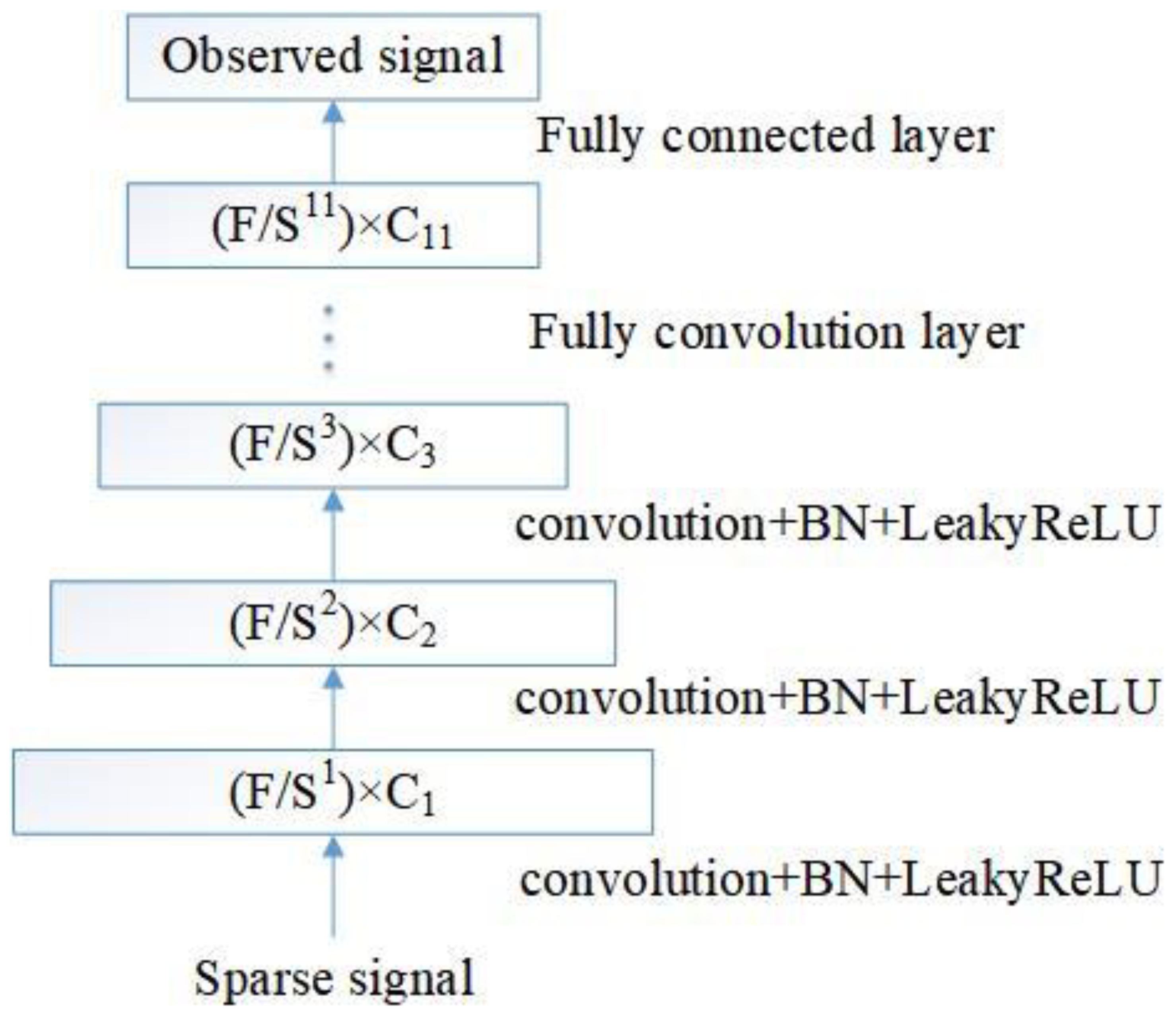
The measurement model is a convolutional neural network (CNN), which is used to observe the gradient signal in X-dimension reduction. The input is the sparse gradient signal, and the feature vector of the specified observation dimension is obtained through eleven convolutional layers and one fully connected layer. The block diagram of the model is shown in Figure 5, where S represents the convolutional step length, and the S of each convolutional layer is 2. C_i represents the number of channels after the signal passes through each convolutional layer, and the corner mark i represents the index number of the convolutional layer (i.e., 1–11). F represents the input gradient signal length and, after convolution, the eigenvector dimension of each layer is F/S_i. After the convolution of the last layer, the feature graph of 8 × 1024 dimensions is obtained, which is input to the fully connected layer through linear smoothing, and the output dimension of the fully connected layer is determined by the observed dimension. The activation function in the measurement model was selected as LeakyReLU, and the batch normalization module (BN) was added, to prevent gradients and disappearances before the activation function.

4. Experimental Results and Analysis

In order to verify the effectiveness of the adversarial transfer federated learning framework proposed in this paper, we obtain user load data from OpenEI, an open dataset for power analysis. The dataset includes hourly residential load data for 24 locations in New York State in 2012. Each location is made up of data for three types of houses, based on their typical patterns of electricity consumption: low, medium, and high. Half of the data are masked randomly, to mimic the DER load collected from the client in real cases.

In this experiment, the mean absolute percentage error (MAPE) and the root-mean-square error (RMSE) were used to evaluate the model performance, and the R² was added to reflect the overall fit degree of the prediction model, where A_t represented the actual load, and F_t represented the predicted load.

$$MAPE=\frac{1}{n}{\displaystyle \sum _{t=1}^n\left|\frac{A_t-F_{\mathrm{t}}}{A_t}\right|}$$

(11)

$$RMSE=\sqrt{\frac{1}{n}{\displaystyle \sum _{i=1}^n{\left(A_t-F_t\right)}^2}}$$

(12)

$$R^2=1-\frac{{\displaystyle \sum {\left(A_t-F_t\right)}^2}}{{\displaystyle \sum {\left(A_t-{\overline{A}}_t\right)}^2}}$$

(13)

In the FL experiment, the deep learning server was configured with an Inteli-9900k CPU and an RTX3080Ti GPU, and the development environment was Ubuntu 16.04, TensorFlow 2.0.0, and Python 3.7. A long short-term memory neural network (LSTM) is used as the target model for load prediction on the local server. The processed load data were used to train the prediction model, and the model was deduced on the test set. The training results were shown as Figure 6.

It can be seen from the figure that the accuracy of the prediction results of the FL model is not ideal. Due to the influence of the mask load, the global model cannot accurately predict the load change in time when facing the influence of non-human factors (weather, climate). Therefore, the adversarial federated transfer framework proposed in this paper is used to train the load data under the same FL client configuration. The prediction results are shown in Figure 7.

Through the adversarial transfer processing of the mask load, the accuracy of the improved prediction model is significantly improved, and the data filling process in the data preprocessing stage is reduced. It can effectively cope with the situation wherein the current DER penetration rate is constantly increasing, and the power load data are significantly masked. By changing the proportion of the mask load in the load data, the predictive advantage of the adversarial federated transfer learning system proposed in this paper is verified in the DER environment. The comparison of the MAPE of different prediction models is shown in

Table 1. Error comparison under different training sets.

	Masked Load (20%)		Masked Load (30%)		Masked Load (50%)
	FL	This Work	FL	This Work	FL	This Work
Dataset 1	7.69	4.41	10.94	5.17	16.59	7.26
Dataset 2	9.24	4.98	12.03	5.15	17.28	7.31
Average	8.47	4.70	11.49	5.16	16.93	7.29

.

The adversarial federated transfer learning training method proposed in this paper can significantly improve the accuracy of mask load prediction. It can be observed that when the mask load accounted for 20% and 30% of the total load data, the MAPE of the prediction model was reduced by 6.7% compared with the traditional FL [25,26]. And when the mask load was increased to 50%, the average MAPE was reduced by 9.6%. In order to highlight the significance of the proposed scheme, the accuracy evaluation indexes of the prediction models are compared in

Table 2. Comparison of model performance with traditional FL.

	MAPE (%)	RMSE (kW)	R2
This work	7.29	1.96	0.89
FL	16.93	4.27	0.74

.

The adversarial FTL proposed in this paper has a higher regression fitting degree. It is proven that the method can be applied in the case of significant-masked-load data.

A DDTCS algorithm is proposed to solve the problem of the high communication cost. The stages of the separate experiments are as follows. Anomaly detection tasks commonly used in the field of machine learning are used as experimental simulation cases. The deep learning framework based on Pytorch version 1.10 is adopted, and the Pysyft library is used to train the federated learning model. The NSL-KDD dataset and UNSW_NB15 dataset, which are widely used in the performance testing of abnormal traffic detection algorithms, are used. Among them, the NSL-KDD dataset is a public dataset provided by the Canadian Cyber Security Institute for network-security-based intrusion detection, and UNSW_NB15 is a public dataset created by the Canberra Network Range Laboratory of the University of New South Wales for network abnormal traffic detection.

For the local computation of model training on each client, the initial learning rate of the stochastic gradient descent (SGD) algorithm with a batch size of 20 is 0.01. Experiments are performed on different sparse thresholds. The accuracy and communication times of different th values are compared. The accuracy (Acc) was used to evaluate the accuracy of the DDTCS algorithm, and the compression ratio (CR) was introduced to measure the effect of the gradient compression. The CR reflects the degree of gradient compression, and is defined as the ratio of the number of gradient exchange communications after compression to the number of communication before compression, under the condition that the target task prediction accuracy is achieved. The lower the compression ratio, the higher the compression degree. In general, reducing the compression ratio can greatly reduce the frequency of gradient communication, and can effectively reduce the communication overhead. But, similarly, a reduction in the compression ratio will also lead to a decrease in the model detection accuracy. Therefore, in order to balance these two indicators, this paper introduces the compressed composite index (CCI) to make the best decision for the model, by adjusting the proportion of the two key indicators. The CCI is defined as:

CCI = β1 × Acc + β2 × (1 − CR)

(14)

Among them, β1 and β2 were used to measure the ratio of Acc and CR for two parameters, β1 + β2 = 1, and β1 > 0, β2 > 0. As the final task of the machine learning model in this paper is abnormal traffic detection, the priority of Acc needs to be higher than that of CR; that is, β1 > β2. The evaluation index CCI of model gradient compression comprehensively considers the Acc and CR. The higher the CCI, the better the overall effect of the model gradient compression.

Table 3. The detection accuracy and compression rate of the model under different th values.

th	Number of Times before Compression	Number of Times after Compression	Average Accuracy	Compressibility (%)
1%	400	391	0.9543	98
5%	400	317	0.9321	80
10%	400	30	0.9122	7

is a comparison between the accuracy rate and the communication frequency obtained via experiments with different values for the sparse threshold th. With the increase in th, the average communication frequency of the model continues to decrease, and the interference in the detection accuracy of the model also increases, and the average detection accuracy decreases slightly in general, with little difference. This makes it possible to further compress the data, by setting a dynamic sparse threshold.

Further, it is necessary to calculate the comprehensive compression index (CCI) of the model under th value. Defined by Formula (14), CCIs with different values for the parameter coefficients β1 and β2 are calculated, respectively, and the results are shown in Figure 8.

Finally, through comparison between the DDTCS algorithm proposed in this paper and the traditional compression sensing CS and the deep compression sensing deep CS, the performance comparison results of each algorithm are shown in

Table 4. Performance comparison of each algorithm under different validation indexes.

Experimental Verification Index	CS	Deep CS	DDTCS
ACC (Train set)	0.789	0.912	0.954
CR (%)	8.732	5.541	8.000
CCI (β1 = 0.4, β2 = 0.6)	0.902	0.923	0.941
CCI (β1 = 0.5, β2 = 0.5)	0.911	0.929	0.947
CCI (β1 = 0.6, β2 = 0.4)	0.901	0.921	0.940

from the three indexes of accuracy, compression ratio, and compression composite index. As can be seen from Table 2, when β1 = 0.5 and β2 = 0.5, the DDTCS algorithm can achieve the maximum CCI value in the same period, and is better than the deep CS algorithm. Although the deep CS can achieve a better compression index, its detection accuracy is significantly different from the DDTCS, which is contrary to our anomaly detection goal. Compared with the traditional federated learning model, the communication cost is further saved by 23.5%; that is, the gradient communication rounds are reduced, but the accuracy is only reduced by 0.26%, which is very small for the federated learning model, which needs to deal with a large number of devices.

5. Conclusions

In this paper, an adversarial federated transfer learning system is proposed to solve the problem of the load data mask in NPSs. The common feature vector between the global model and the local data are extracted through adversarial training, so as to compensate for the loss of mask load in the prediction accuracy, and improve the prediction accuracy. The traditional FL model compression algorithm is improved, and a compression sensing method based on a depth dynamic threshold is proposed, to greatly reduce data redundancy and ensure efficient communication. Finally, through experimental analysis, the effectiveness and feasibility of the proposed scheme are verified. Compared with traditional FL, adversarial transfer training can effectively improve prediction accuracy, and reduce the average MAPE by 9.6% and RMSE by 2.31 kW, when the load data are masked to different degrees. Compared with the traditional FL model, the proposed DDTCS compression algorithm reduces the communication cost by 23.5%, while ensuring the accuracy of the model is only slightly reduced, by 0.26%.