Prediction of the Electricity Generation of a 60-kW Photovoltaic System with Intelligent Models ANFIS and Optimized ANFIS-PSO

Abstract

The development and constant improvement of accurate predictive models of electricity generation from photovoltaic systems provide valuable planning tools for designers, producers, and self-consumers. In this research, an adaptive neuro-fuzzy inference model (ANFIS) was developed, which is an intelligent hybrid model that integrates the ability to learn by itself provided by neural networks and the function of language expression, how fuzzy logic infers, and an ANFIS model optimized by the particle swarm algorithm, both with a predictive capacity of about eight months. The models were developed using the Matlab^® software and trained with four input variables (solar radiation, module temperature, ambient temperature, and wind speed) and the electrical power generated from a photovoltaic (PV) system as the output variable. The models’ predictions were compared with the experimental data of the system and evaluated with rigorous statistical metrics, obtaining results of RMSE = 1.79 kW, RMSPE = 3.075, MAE = 0.864 kW, and MAPE = 1.47% for ANFIS, and RMSE = 0.754 kW, RMSPE = 1.29, MAE = 0.325 kW, and MAPE = 0.556% for ANFIS-PSO, respectively. The evaluations indicate that both models have good predictive capacity. However, the PSO integration into the hybrid model allows for improving the predictive capability of the behavior of the photovoltaic system, which provides a better planning tool.

1. Introduction

Electrical energy generation with hydrocarbons accounts for about 38% of global CO₂ emissions [1]. A Life cycle analysis of photovoltaic plants shows that CO₂ emission rates are significantly lower than those of systems using fossil fuels. Therefore, photovoltaic systems have a significant potential to mitigate global warming [2,3]. The virtuous circle of technological development, innovations in design, and the joint action of nations have been decisive in reducing the costs of generating electricity through photovoltaic technology [4]. The progressive decrease in large-scale solar PV generation prices fell by 85% between 2010 and 2020, from USD 0.381 per kWh to USD 0.057 per kWh [5]. It has driven an increase in the installed capacity of photovoltaic solar energy (PV) generation, with an annual growth rate of 38.3% since 2009. Solar photovoltaic energy achieved the most significant capacity increase ever seen in a single year, in which the annual rate increase was 21.5% in 2020 compared to 2019 [6]. By 2020, producing electrical energy through PV systems would represent only 2.7% of the world’s electrical generation [5]. However, in sustainable development, projections estimate that, in approximately 40 years, 60% of global electricity generation will be generated by solar technologies [7].

Since solar power generation technologies are subject to operational intermittencies according to the hours of the day and local meteorological conditions [8,9], prediction techniques are a valuable tool in the planning, designing, and operating of photovoltaic systems [10]. Predictive models based on artificial intelligence provide a productive use of analyzing geographic and meteorological conditions in the study sites [11,12] and an innovation in the relationship between computational methods, data mining, and optimization methods based on observations of nature [13,14]. The particular meteorological conditions that occur in the operating sites of the PV systems are relevant since variations more significant than expected can cause fluctuations in the output power of the system [8,15,16], which is why the appropriate recording and historical analysis of the meteorological variables, as well as the electrical generation of the system, is essential in the feeding and training of the predictive models [17,18,19].

Due to the exponential growth scenario of the use of photovoltaic generation energies [20] and the variability in their generation [16], it is of essential importance to know the behavior of their productive capacity, which is key for an efficient annexation to the electrical network. Therefore, implementing techniques that allow building predictive models of electricity generation has boomed in recent years; using an adequate methodology for recording experimental data and implementing intelligent computer models can provide a good forecasting capacity for electricity generation [21,22].

A wide variety of research has been developed in recent years on this topic, from those that use statistical forecast models to those that use forecast models based on the use of artificial intelligence, hybrid models, and even those that implement optimization methods inspired by observations of nature, with which they seek to improve the predictive capabilities of the models. Zhu et al. [23] presented an investigation where they collected monthly electricity generation data from 2001–2020 in the province of Xinjiang, China. The objective focused on predicting electricity generation using the Holt–Winter statistical models and the mean model autoregressive integrated mobile (SARIMA), obtaining monthly forecasts for 2021–2022, and determining where the SARIMA model showed less error in the approach to the evaluated experimental data. Xu et al. [24] presented a predictive study on future renewable energy trends. They developed predictions using the differential autoregressive integrated moving average (ARIMA) models, the neural network model, and the support vector machine model. Later, the authors combined the previous three, building a fourth hybrid model and achieving this reduced error in the predicted value.

Wang et al. [25] presented a very short-term prediction model of the energy generated by a photovoltaic system, combining three methods, variational modal decomposition (VMD), to decompose the sequence of historical photovoltaic power into different segments. They implemented the grid prediction model of long short-term memory (LSTM) and the relevance vector machine (RVM) model to predict the error sequence. Combining these methods improved energy prediction on the five simulated days, obtaining MAPE values between 2 and 3% for periods with little historical meteorological variability. Comert et al. [26] presented a study to estimate the monthly solar radiation values of six weather stations with different radiation indices in Turkey, comparing the empirical angstrom, Hargreaves–Samani equations, artificial neural network (ANN), machine learning models of support vectors (SVM), and LSTM, concluding that the latter achieved a better predictive capacity.

Pazikadin et al. [27] presented an extensive literature review of 87 research articles from the period 2014 to 2019 on the implementation of different types of artificial neural networks (ANN) in the prediction of solar energy and the importance of proper instrumentation calibration in the collection of meteorological data, which, depending on its optimal quality, can help the ANNs improve their precision. Buturache and Stancu [28] presented a study on the fundamentals of applying meteorological data in designing predictive solar and wind energy models based on standard recurrent neural network models and long-term memory terms. They closed recurring units and developed their fundamentals and comparisons in predictive periods within one hour.

Patel et al. [29] carried out a systematic study of the prediction of solar irradiation and solar PV generation and carried out a detailed analysis of ANN models, such as those based on the backpropagation algorithm, multilayer forward algorithm, and linear regression, in addition to hybrid models based on fuzzy logic, analyzing the behavior with various input parameters and different layer structuring, concluding that hybrid models based on ANN and fuzzy logic have a better predictive capacity. Dokmen et al. [30] developed three intelligent models based on the wavelet artificial neural network (WANN), wavelet support vector machine (WSVM), and ANFIS to estimate solar energy at two stations in Iraq. The results were compared to experimental data and evaluated with statistical criteria, resulting in satisfactory predictive results for all three models, with a slightly better predictive ability for WANN for the two sites.

Perveen et al. [31] developed an ANFIS model to predict short-term power generation with applications in a smart grid using variables from a composite climate zone. Finally, the results were compared with other predictive models such as ANN, vector machine, and fuzzy logic, with the ANFIS model obtaining the best results. Sujil et al. [32] proposed an ANFIS predictive model for forecasting the output power of a photovoltaic system and a wind system for a power management system in South China. The ANFIS model was developed with three different partitioning techniques, compared with the backpropagation algorithm, and later evaluated with statistical methods, resulting in ANFIS fuzzy c mean clustering with better results for both algorithms. Viswavandya et al. [33] developed two predictive models based on fuzzy logic and ANFIS, respectively, where they used historical meteorological data to predict short-term solar irradiation and then compared them with on-site historical radiation data, reporting satisfactory results. Haji and Genc [34] proposed a maximum power point tracking (MPPT) controller for an off-grid photovoltaic system based on the ANFIS, Perturbation and observation (P&O), and fuzzy logic controller (FLC) to track the maximum power point, concluding that the ANFIS shows better tracking efficiency, lower ripple power, and resistance to system voltage and current changes.

In recent years, a large amount of research has been conducted on computational methods of combinatorial optimization [18,35], where optimization algorithms are used in the search to improve the capacity of predictive models. Combinatorial optimization [36] improves their ability to address complex and non-linear problems [37], and coupling has been successfully applied in various fields of science [38,39,40,41]. Slowik and Kwasnicka [42] extensively studied evolutionary algorithms such as genetic algorithms, genetic programming, differential evolution, evolution strategies, and evolutionary programming, their nature, properties, and selective application in different areas of engineering. Khosravi et al. [43] developed an optimized ANFIS model with a hybrid of genetic algorithm and teaching–learning optimization algorithm (ANFIS-GATLBO) to evaluate central tower solar systems with thermal storage, using the general parameters of their design depending on each geographical region and comparing it with the artificial neural network and FIS models, resulting in ANFIS-GATLBO being more accurate in the results.

Ndiaye [44] implemented an intelligent predictive model, ANFIS, and an optimized model, ANFIS-GA, to predict the power generated by a photovoltaic system and distribute it to the national electricity grid in Senegal. The results determined that ANFIS-GA was more efficient, obtaining a mean square error of 2.027 W compared to ANFIS, which obtained 4.142 W. Lara-Cerecedo et al. [45] developed the intelligent models ANFIS and ANFIS optimized with a genetic algorithm and carried out a comparative study of their efficiency in the prediction of electrical energy generated from a photovoltaic system in northwestern Mexico. The variables of ambient temperature and solar radiation were evaluated with statistical methods, concluding that the optimized ANFIS-GA model obtained better results with a MAPE of 4.56% compared to the ANFIS model, which obtained a MAPE of 6.98%. Slowik and Kwasnicka [46] presented an investigation regarding swarm intelligence algorithms based on natural collective intelligence. The objective was to describe the mathematics of its operation and its application in various industries and economic sectors. Khosravi et al. [47] developed two predictive models, ANFIS and ANN, which were optimized with GA, and independently, the same two models were optimized with PSO to simulate the energy and thermal behavior of a Stirling solar collector. They used different meteorological and geometric variables and collector designs for all models. ANFIS optimized with PSO reported the best results.

Wu et al. [48] presented a hybrid model based on the Elman neural network (ELM) and the adaptive network-based fuzzy inference system (ANFIS), which in turn was optimized with the parasitism–predation algorithm to improve the short-term prediction of energy demand obtained from the consumption statistics of November 2020. Its results were evaluated with statistical methods. They determined a better substance in the daily predictive capacity of the optimized hybrid model compared to the non-optimized hybrid, decreasing the RMSE by 48.4%, the MAE by 46.0%, and the MAPE by 47.4%. Ghenai et al. [49] developed an ANFIS model to predict energy consumption in the very short term (0.5, 1, and 4 h) at the University of Sharjah campus, Sharjah, United Arab Emirates, where their results were very accurate at the 30-min horizon, reducing its estimation approach as the estimation took a longer amount of time to predict, concluding that the model requires a large amount of data collected to be able to carry out training that allows the predictive horizon to be extended without a greater margin of inaccuracies. Eya et al. [50] presented an improved ANFIS predictive model for the estimation of the weekly and monthly load consumption for six months of the electrical system of the University of Nigeria, Nsukka. For its design and training, they carried out a collection of historical environmental and consumption data during the period 2014 to 2019. The predictive data were statistically evaluated, obtaining MAPE values below 5%. Yang et al. [51] presented a short-term novel predictive model for the electricity demand of New South Wales in Australia. This model combines three models based on the back propagation (BP) neural network and the adaptive network-based fuzzy inference system (ANFIS) to adopt the advantages of handling data regarding linearity, non-linearity, and seasonality of the individual models. A Differential Evolution (DE) optimizing algorithm was added to improve its precision. They compared the results with the experimental data on electrical demand for half an hour, giving the combined model a better approach than the three individual models.

Ashari [52] developed an ANFIS-PSO model that allows for the best configuration of an MPPT controller. The performance was compared with the perturb and observe algorithms (P&O) and incremental conductance (Inc). The efficiency of an ANFIS-PSO showed that it worked better than the other algorithms and reached 98.36% under standard test conditions. Adedeji et al. [53] developed a PSO-optimized ANFIS model for short-term wind turbine power production forecasting in the Cape, South Africa. The study addressed the importance of data binning in predictive models using grid partitioning (GP) techniques, subtractive clustering (SC), and fuzzy-C-means (FCM), evaluating the SC with better statistical measurements.

The literature survey showed various studies on predictive intelligent models and their usefulness in broad engineering and science areas. Also showed interest in implementing new optimization techniques that help improve the robustness and accuracy of the model’s predictions. We observed that few studies have explored how these models should be complemented, and even fewer have rigorously compared the results of different models. The literature analysis indicated the absence of investigations related to predicting the energy production of photovoltaic systems using neuro-fuzzy adaptive systems coupled to a particle swarm optimizer algorithm that performs not only the predictions of electrical power but also the predictions of electric energy generation, which is essential for the economic analysis of photovoltaic plants. Therefore, the main objective of this research was the development of two models, ANFIS and the optimized ANFIS-PSO model, that used experimentally captured data for their training and allowed us to make predictions over a window of almost eight months for both models. Each model has processed and learned from around 225,400 pieces of data per variable and was able to present very accurate predictive results. In addition, the algorithms showed great flexibility to deliver predictions for arbitrary periods and showed predictive robustness under volatile weather situations. A comparison was made between both models using statistical indicators widely used in the literature. The ANFIS system obtained RMSE values in the test segment: 1.79 kW, RMSPE: 3.075, MAE: 0.864 kW, and MAPE: 1.47% compared to the ANFIS-PSO, which obtained RMSE: 0.754 kW, RMSPE = 1.29, RMSPE: 1.29, MAE: 0.325 kW, and MAPE: 0.556 %, respectively. The above showed the predictive superiority of the optimized model.

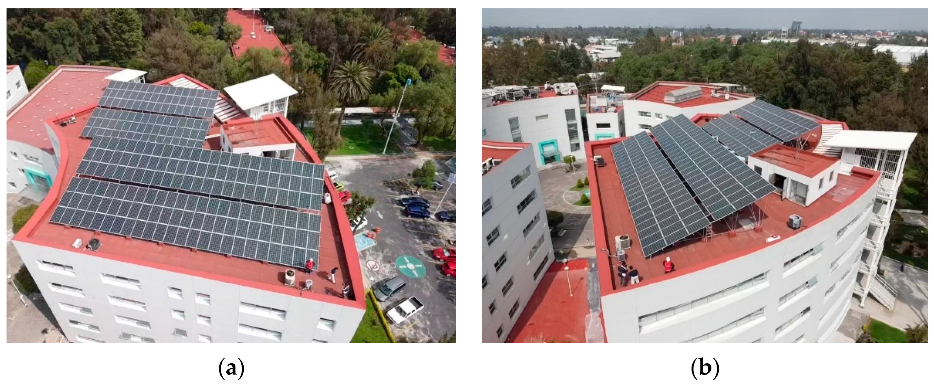
2. Experimental Setup and Data Processing

The present research is based on the study of a photovoltaic system located at the Center for Research and Advanced Studies of the National Polytechnic Institute (CINVESTAV-IPN) in Mexico City, Mexico (latitude 19°30′48′′ N and longitude 99°07′57′′ W). The photovoltaic array consists of 240 monocrystalline silicon photovoltaic modules of the brand Solartec (model S60MC, Guanajuato, Mexico), mounted on an aluminum structure with an orientation of 30° in azimuth towards the East of the geographic South and at an angle of inclination of 20°. Each module has a nominal power of 250 W and a high cell efficiency of up to 15%, for a total cumulative capacity of 60 kW. Figure 1 shows the photovoltaic system.

The photovoltaic module array is subdivided into five sections. Each section comprises a chain of 48 modules, with 12 connections in series and 4 in parallel. The nominal power of each section is about 11.9 kW. The system has one inverter of the Fronius brand. IG Plus V11.4.2 DELTA (Pettenbach, Austria): It has a capacity of 11.4 kW per section and a maximum efficiency of 96.2%. The system has a thermopile-pyranometer EKO MS-602 (Tokyo, Japan) installed at an angle of 20° from the horizontal, whose technical characteristics are: spectral Error: ±0.2%, temperature response (−20 °C to 50 °C): ±2%, wavelength range (nm): 285 to 3000, irradiance range (W/m²): 0 to 2000, operating temperature: −40 to 80 °C, calibration traceability/uncertainty: ISO 17025/WRR/<0.7% (k = 1.96), and an anemometer installed on-site to measure wind speed. Figure 2 shows the support PV system instruments.

Lastly, each data logger records and integrates the system’s weather and power variables every 5 min, 24 h a day. The registered variables are wind speed (m/s), module temperature (°C), ambient temperature (°C), solar radiation (kWh/m²), and system output power (kWp), which were used as variables of the intelligent model. The design of the smart algorithm, record analysis, training, and predictive testing were done on a laptop with a CPU i3-1005G1 and 8 GB of RAM.

As a first step, information processing (collection, extraction, storage, structure, and analysis) was carried out due to the large number of records collected. The data was extracted from historically collected data files and distributed according to the time sequences of each of the input and output variables stored. Secondly, due to the need to determine the level of influence of each input variable concerning the electrical generation of the system, a correlation analysis of each input variable concerning the output variable was made. The research helps to describe the association between quantitative and categorical variables, where the associated variables change in tandem [54]. About 225,441 records per variable for approximately 26 months were used. The Pearson correlation coefficient (Equation (1)) was used, as well as Spearman’s correlation coefficient (Equation (2)), which are explained in [55]. The results obtained from the correlations are shown in

Table 1. Correlation of the input variables concerning the output variable generated power of the PV system.

Input Variables	Power (kW)
	Coefficient	Correlation	R2
Global horizontal solar radiation	Pearson	0.997	0.994
Module temperature	Pearson	0.94	0.88
Ambient temperature	Pearson	0.86	0.74
Wind speed	Spearman	1.16	1.35

.

$$r_p=\frac{\sum d_x{d}_y}{\sqrt{\sum d_x^2\sum d_y^2}}$$

(1)

$$r_s=\frac{1-6\sum d_i}{n(n^2-1)}$$

(2)

where, $r_p$ is the Pearson’s correlation coefficient, $\sum d_x{d}_y$ is the product sum of squares, $\sum d_x^2\sum d_y^2$ are the sum of squares of $X$ and $Y$respectively, and $r_s$ is the Spearman’s correlation coefficient, $d_i=X_i-Y_i$ is the variation in the rankings of the corresponding variables, and $N$ is the number of observations.

The results of the models were evaluated under strict statistical metrics whose mathematical formulations were found and adapted from the literature [56,57]. The statistical methods used to assess the efficiency of the models were the root mean square error (RMSE), the root mean square percentage error (RMSPE), the mean absolute error (MAE), and the mean absolute error in percent (MAPE), where Equations (3)–(6) were used, respectively. RMSE (Equation (3)) is a quadratic evaluation mechanism measuring errors’ mean magnitude. Where, $d_i$ is the predicted values and $y_i$ are the observed values, and $n$ is the number of observations.

$$RMSE=\sqrt{\frac{1}{n}\sum _{i=1}^a{(d}_i-{y_i)}^2}$$

(3)

However, RMSPE (Equation (4)) calculates the square root of the average of the squared percentage errors. It has the same properties as RMSE, with the difference that the results are expressed in percentages. Where, $n$ is the number of samples, $y_t$ is the current value, and $\widehat{y_t}$ is the estimate. The loss function of the measure is the error squared.

$$RMSPE=\sqrt{\frac{1}{n}\sum _{t=1}^n{\left(\frac{y_t-\widehat{y_t}}{\left|y_t\right|}\right)}^2}$$

(4)

MAE (Equation (5)) provides a generic and bounded performance measure for the model. Corresponds to an estimate of the absolute error. This level indicates the average magnitude of the true and predicted values. Where ${\widehat{Y}}_i$ is the estimated value, $Y_i$ is the present value, and $N$ is the number of simples. As MAE approaches zero, the model is considered more accurate.

$$MAE=\frac{1}{N}\sum _{i=1}^N\left|Y_i-{\widehat{Y}}_i\right|$$

(5)

MAPE (Equation (6)) determines the percentage accuracy compared to the true value. Where $n$ is the number of fitted points, $A_t$ is the actual value, $F_t$is the forecast value, and Σ is the summation notation (the absolute value is summed for each point in the forecast time).

$$MAPE=\frac{1}{n}\sum _{t=1}^n\left|\frac{A_t-F_t}{A_t}\right|$$

(6)

3. Methodology of the Predictive Models

3.1. ANFIS Model

An ANFIS system is a multilayer direct-feed network formed by neurons associated with connections. The construction process of the hybrid model was based on five layers. Which have been widely studied and are adapted from [32,58,59,60]. Using the least squares method, ANFIS performs a forward propagation to obtain the consequent parameters $p_i$, $q_i$, $r_i$ indicated in Equation (10), in the defuzzification layer and uses the backpropagation algorithm to minimize errors through gradient descent and thus modify the premise parameters $a_i$, $b_i$, $c_i$ indicated in Equation (7), in the fuzzification layer.

Layer 1. In the first layer, the fuzzification is carried out. In this process, the neurons transfer the previously received signals according to their encoding, which can be a square node with a square function. Each neuron can generate a value belonging to a linguistic level.

$$O_i^1=\mu A_i\left(x\right),fori=1,2,3=\exp \left[-{\left({\left(\frac{x-c_i}{a_i}\right)}^2\right)}^{b_i}\right]$$

(7)

where, $O_i^1$ denotes the output function and $\mu A_i$ denotes the membership function, and $x$ is the node input, wherein a, b, and c are used to represent the membership function’s shape-altering premise parameters.

Layer 2. This layer is called the rules layer because the weights of the membership functions are computed. The rules layer represents the activation force of each rule generated in the fuzzification layer.

$$O_i^2=\mu A_i\left(x\right)\times \mu B_i\left(y\right),i=1,2,3$$

(8)

Layer 3. The fuzzy rules are determined, and the beginning of each of them is calculated.

$${O_i^3=w}_i=\frac{w_i}{w_1+w_2},i=1,2,3$$

(9)

where, $O_i^3$ represents the output of the normalization layer and $w_i$ the normalized firing force.

Layer 4, called a defuzzification layer. In this layer, the output values are calculated considering the trigger strength values from earlier layers.

$$O_i^4={\overline{w}}_i{f}_i={\overline{w}}_i(p_{i}x+q_{i}y+r_i)$$

(10)

where, ${\overline{w}}_i$ represents the output of layer 3, and the set of parameters called consequents are $p_i$, $q_i$ y $r_i$.

Layer 5. In this layer, the total output is calculated as the sum of all the previous signals. The output value has a value of a continuous type instead of a fuzzy set type.

$$O_i^5=\sum _i{w}_i{f}_i=\frac{{\sum }_i{w}_i{f}_i}{\sum _i{w}_i},i=1,2,3$$

(11)

Figure 3 shows an ANFIS structure with four inputs and one output. The model is composed of five layers, which are subdivided into the premise part and the consequent part.

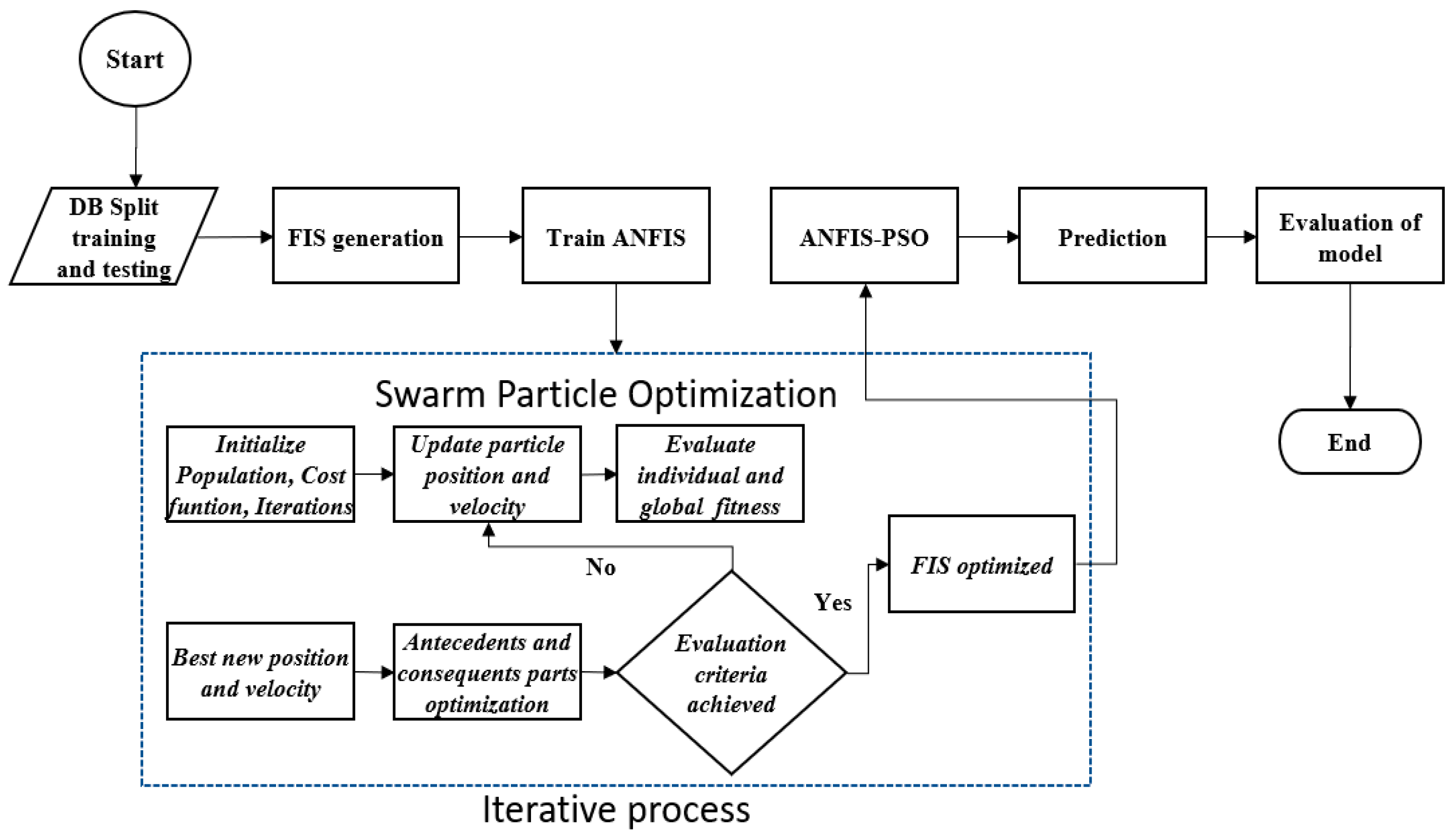
3.2. ANFIS Optimized with Swarm Intelligence Algorithms

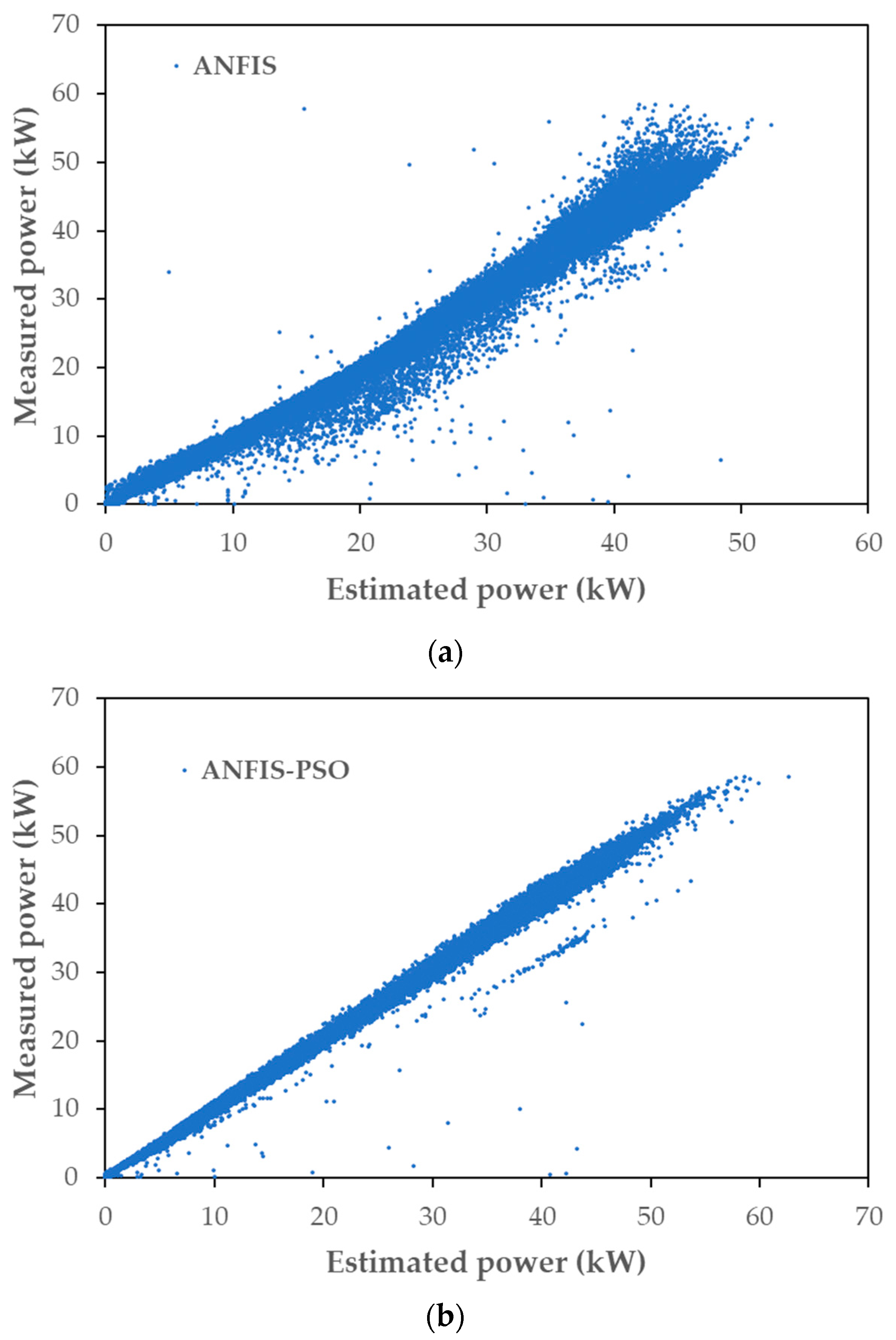
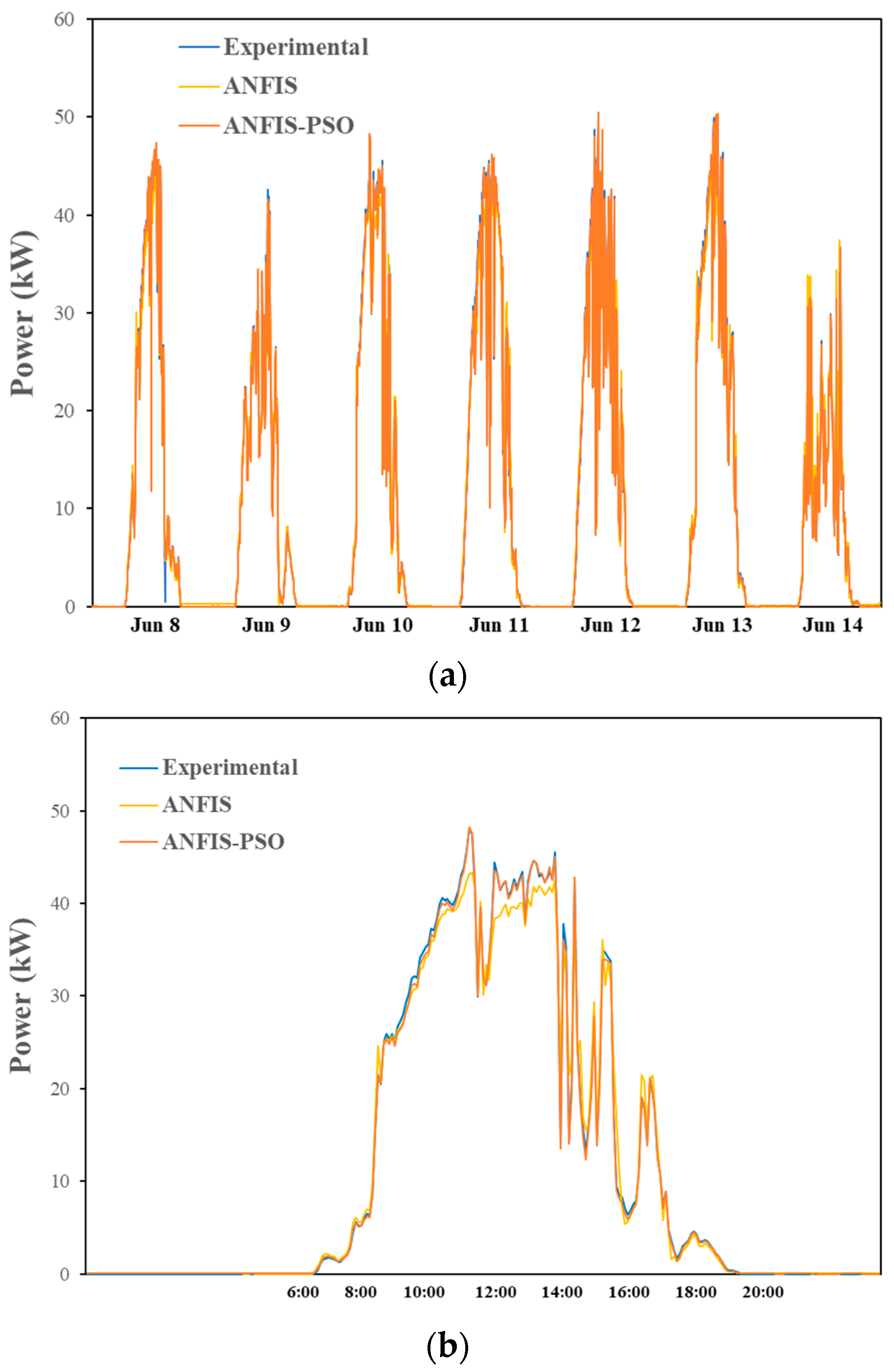
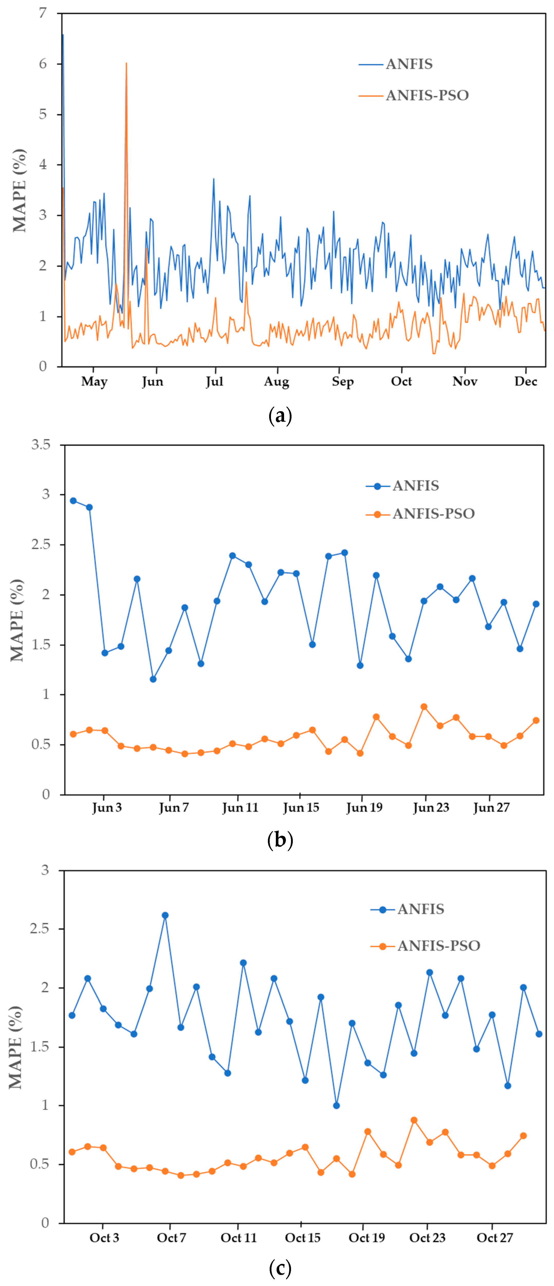
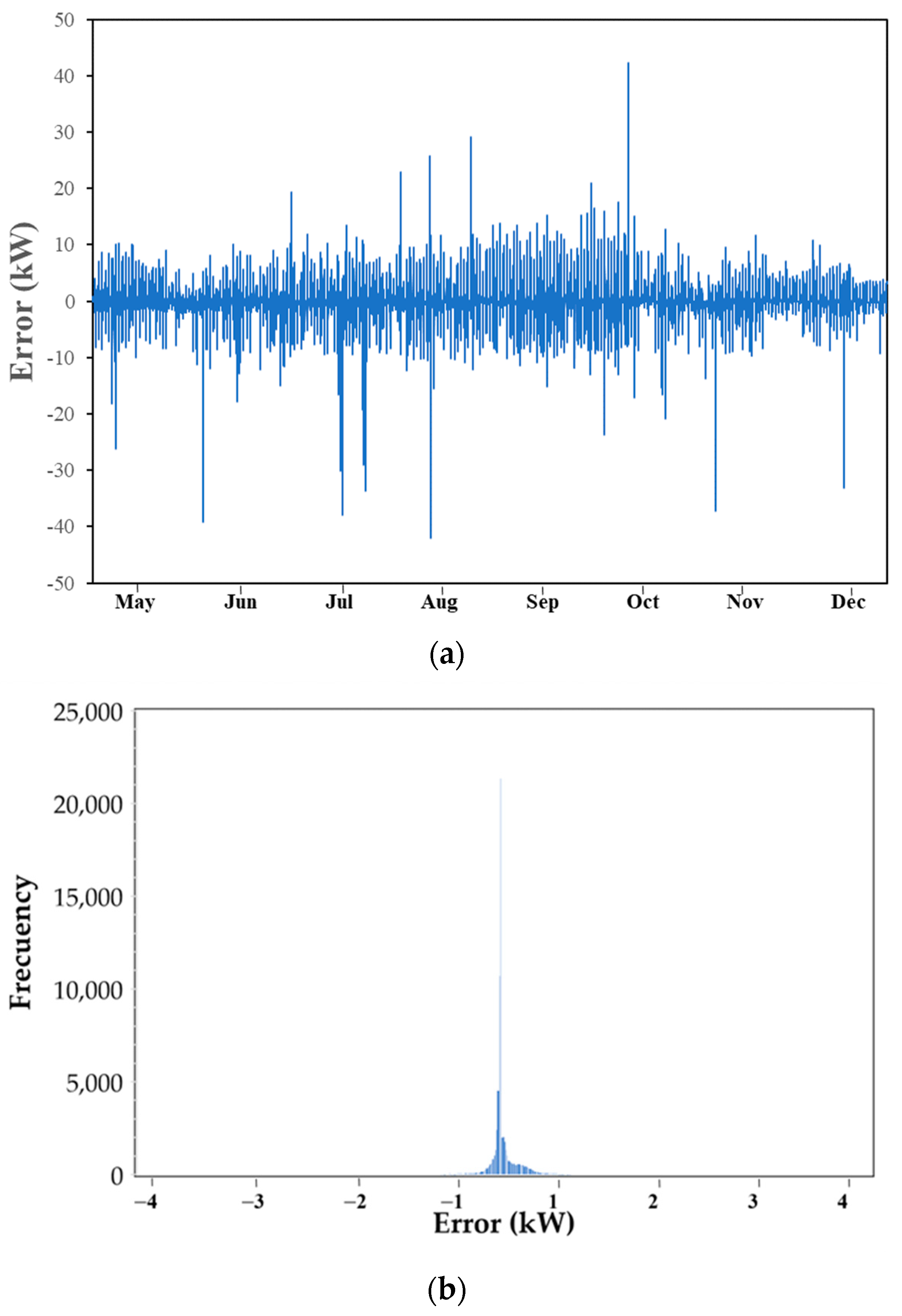
Evolutionary computing is an area of artificial intelligence that investigates optimization algorithms based on nature [61]. They look for solutions based on trial and error, using stochastic optimization, and provide tools to solve complex engineering problems involving randomness and non-linear dynamics [62].

Particle swarm optimization (PSO) is a branch of computational intelligence [63] that can be used as a global optimization technique where, through heuristic optimization, it seeks to find global minimums or maximums [64]. The operation is based on the swarm intelligence observed in nature as the behavior of groups of fish or birds, where the movement of each member is the result of combining individual decisions with the behavior of the rest, perceived as collective intelligence [46]. In the PSO, each moves in the search space according to a mathematical formulation, with a dynamically adjusted speed based on his own experience and his partner’s experience. Each one is a point in the search space that uses their expertise to find their best position, and the social knowledge of the group helps to determine the best place of the entire swarm, the global minimum or maximum. The PSO process is adapted and widely explained in [46,65,66,67].

The algorithm starts the swarm $P(t)$, where the position $\overrightarrow{x_i}($t$)$ of each particle is random in all space, and then the performance F of each particle is evaluated using the current position $\overrightarrow{x_i}(t)$, where the speed and position of the particle are given by Equations (12) and (13).

$$V\left(t\right)=V\left(t-1\right)+c_1·r_1·\left(P_{best}-X\left(t-1\right)\right)+c_2·r_2·\left(G_{best}-X\left(t-1\right)\right)$$

(12)

$$X\left(t\right)=X\left(t-1\right)+V(t)$$

(13)

where, $V(t)$ and $X(t)$, are the velocity and position of the particle, $P_{best}$ is the induvial best value and $G_{best}$ is the global best value up until the most recent iteration, $r_1\mathrm{a}\mathrm{n}\mathrm{d}{r}_2$ are random in the 0–1 range, and t finally $c_1\mathrm{a}\mathrm{n}\mathrm{d}{c}_2$ are coefficients of particle acceleration.

Subsequently, the performance of each individual is compared with their best performance so far, such that if $\overrightarrow{f(\overrightarrow{x_i}}(t))<{pbest}_i$, then ${pbest}_i=\overrightarrow{f(\overrightarrow{x_i}}(t)),$consequently, the performance of each individual is compared with the best global particle, such that if $\overrightarrow{f(\overrightarrow{x_i}}(t))<{gbest}_i$, then ${gbest}_i=\overrightarrow{f(\overrightarrow{x_i}}(t)).$ In addition, the velocity vector change is performed for each one using Equation (14).

$$v_i\left(t+1\right)={wv}_i\left(t\right)+c_1{r}_1\left[\widehat{x_i}\left(t\right)-x_i(t)\right]+c_2{r}_2\left[g\left(t\right)-x_i(t)\right]$$

(14)

where, $v_i\left(t+1\right)$ is the speed of the particle i at the moment $\left(t+1\right)$, $v_i\left(t\right)$ is the speed of the particle i at the moment t, w is the coefficient of inertia, it reduces or increases to the velocity of the particle, $c_1$ is the cognitive coefficient, $r_1$ is the vector of random values between 0 and 1 of length equal to that of the velocity vector, $\widehat{x_i}\left(t\right)$ is the best position in which particle i has been so far, $x_i\left(t\right)$ is the position of particle i at time t. $c_2$is the social coefficient, $r_2$ is the vector of random values between 0 and 1 of length equal to that of the velocity vector, and $g(t)$ is the position of the entire swarm at time t, therefore the best global value.

Finally, each particle is relocated to its new position according to Equation (15), and the iteration is repeated until convergence. Subsequently, the particle with the worst local value is selected and replaced with a new one with a better value. In such a way, PSO helps optimize the parameters of the antecedent part and the consequent parameters of ANFIS, improving the model’s predictive capacity.

$$\overrightarrow{\overrightarrow{x_i}}(t=\overrightarrow{\overrightarrow{x_i}}\left(t+1\right)+\overrightarrow{\overrightarrow{v_i}}(t)$$

(15)

The ANFIS-PSO model finds the relationship between the input and output data to obtain the optimal configuration of the membership functions. The algorithm uses least squares methods and the back-trapping algorithm that uses the descending gradient method to calculate partial derivatives and thus minimizes errors by adjusting the weights to fit the training data [68,69]. The integration of optimization through PSO aims to improve the classification capacity of ANFIS so that more accurate predictions can be achieved.

In the ANFIS model, the PSO algorithm is mainly used to optimize the parameters of the antecedent layer (layer 1), where the parameters of the fuzzy membership functions are adjusted, and the consequent layer (layer 3), where the optimal values of the weights of the consequent functions are adjusted to obtain a more accurate output. In the PSO algorithm, the particles representing different combinations of parameters move in the search space, updating their velocity and position according to the best individual and global location, looking for the optimal combination of parameters. The dynamics of the PSO process begin by randomly generating a set of particles, where each represents a set of parameters of the ANFIS model (in this case, the weights, and centers of the membership functions). Then begins an iterative process where the model evaluates the fitness of each particle using a performance metric, in this case, the RMSE. Then, based on the PSO equations, the particles are updated to the best individual position, which is those in which the particles have obtained the best fitness until that moment, and the best global position is the position in which some particles have obtained the best fitness. The process continues by updating the velocity and position of each particle. The position is updated based on the current speed. The process is repeated until the criterion of the maximum number of iterations is established, obtaining the best global position, and providing the final parameters of ANFIS. It should be noted that optimizing the ANFIS layer parameters can improve the accuracy and overall performance of ANFIS, which can indirectly impact rule layer two and overall model performance.

However, during the optimization process, the parameters of the membership functions and weights are modified, PSO adjusts the initialized parameters randomly from the first step, and iterative adjustments are made to each parameter until the objective function is reached.

Table 2. PSO initial configuration parameters.

Parameters	Value
Initial population	25
Iterations	1000
Inertia coefficient	1
Personal acceleration coefficient	1
Global acceleration coefficient	2
Damping ratio of the inertial coefficient	0.99
Training population	157,810

shows the PSO parameters of the optimization process. These values can be modified using the trial-and-error method, in which 1000 iterations were used to obtain the best cost, which is measured with RMSE. The objective of the PSO is to help ANFIS optimize the antecedent and consequent parameters.

It is essential to point out that there is no consensus on a single and unified metric for the design of the parameters or an ideal initial configuration of the PSO algorithm that works optimally for all problems. The configuration decision is based on the mathematics of the algorithm and a trial-and-error adjustment in which several optimization tests are performed to select the one that provides the most accurate results possible, seeking to maintain an adequate balance between the results and the computational effort. For example, the swarm size or number of particles, where a larger swarm size may allow a better exploration of the search space but may also increase the computational cost. The inertia coefficient controls the influence of the previous velocity of a particle on its current motion. When it is high, it may favor the initial exploration of the search space, while if it is low, it may favor the exploitation of the best solutions. The personal acceleration coefficient controls the tendency of a particle to move towards its personal best position; the global acceleration coefficient determines the tendency of a particle to move towards the global best position found by the swarm; and the damping ratio of the inertial coefficient is used to gradually reduce the inertial coefficient as the optimization progresses in each iteration. In any case, it is essential to point out that the optimal parameter values may vary depending on the problem and the data type. The selection and configuration of the PSO parameters could even use some other algorithm that seeks, through an iterative process, to find the optimal configuration for a specific case. Figure 4 shows the flowchart of the PSO integration in ANFIS.

The coding and design of the ANFIS hybrid model and the evolved ANFIS-PSO model were carried out using Matlab^® software v2017b. Each model integrated four input variables and a single output variable. A total of 225,442 records per variable were imported into the algorithm. For the model training and testing process, it is essential to segment the total universe for each of the actions. Experimental studies have shown that machine learning models that use 70–80% of the data for training and 20–30% of the data for tests produce the best results [70,71,72,73]. The data from the test set is used to determine the predictive accuracy of the models. The preceding is intended for the model to learn from the data provided with low bias and training error but also to have the ability to generalize new data with low variance and low error in the test segment, that is, to avoid overfitting and underfitting. It is known as the bias and variance dichotomy [74,75].

Poor generalization from data can be characterized by overtraining. If the model overtrains, it only memorizes the behavior of the training data and cannot give correct outputs. The difference between the training and testing errors is too high. On the other hand, it may also present an undertrained. In this case, the model cannot obtain an admissibly low error value in the training segment. Therefore, the model cannot learn well enough from the training mapping, which will result in poor levels of accuracy in the prediction [76].

Empirical training tests were carried out in the evolved ANFIS-PSO model with three data partitions. They were evaluated with the MAPE statistical method, selecting the data segmentation that lowered the percentage error presented (

Table 3. Comparisons of data segmentation scenarios used for the training and testing processes of ANFIS-PSO.

Train (%)	Test (%)	MAPE (%)	Difference (%)
70	30	0.556	0
75	25	0.581	4.5
80	20	0.602	8.28

).

According to the results, 70% of the total data universe was selected for the training stage and the remaining 30% for the predictive phase.

It is essential to highlight that the computational effort registered in each training stage, in the process of 1000 iterations, for the ANFIS model was approximately 625 min, and in the ANFIS-PSO model was about 460 min, reaching the best cost (that in this case, the model measures with the RMSE) for ANFIS of 1.79 and for ANFIS-PSO of 0.747 (

Table 4. Comparison of statistical errors of the ANFIS and ANFIS-PSO models during the predictive stage.

Parameters	Data Statistics
	RMSE (kW)	RMSPE (%)	MAE (kW)	MAPE (%)
ANFIS	1.797	3.07	0.864	1.478
ANFIS-PSO	0.747	1.29	0.325	0.556

). The above represented a better convergence of the model optimized with the PSO algorithm over the non-optimized ANFIS model, reaching a percentage decrease of 35.9% in training time and a decrease in RMSE error of 140%.

4. Results

As previously indicated, the training of the models (training stage) was carried out with 70% of all the recorded data (15 October 2020, to 18 April 2022), representing an accumulated total of 157,809 records per variable collected by the system instrumentation as indicated in the materials and methods section. At the same time, the remaining 30% (predictive stage) was used to carry out the prediction tests (19 April 2022, to 12 December 2022), representing a cumulative total of 67,632 records for predictive tests. The statistical errors between the experimentally recorded PV system power and the estimated results of both models in the predictive stage are presented in Table 4. The optimized ANFIS-PSO model shows a considerable reduction in error evaluation, where we observe a lower average error.

However, the results are presented by comparing the models with the experimental records individually, and then the two models are compared against each other about the experimental data. In Figure 5, the predictive results of the ANFIS hybrid model are plotted against the experimental power records collected from the system from 19 April to 12 December 2022. In Figure 5a, the entire universe of test data was plotted. It was considered necessary since, although visually difficult to analyze in detail, the wide range of predictive capacity that the models presented required. Subsequently, October was selected, where the MAPE result was most satisfactory (Figure 5b), to show the predictive behavior of the model in more detail. Figure 5c shows the month with the lowest MAPE error from 21 to 28 October. In the latter, it is possible to observe the predictive approach of ANFIS in greater detail visually.

Under these same parameters, Figure 6 shows a sequence of graphs of the results of the ANFIS-PSO model against the actual power records of the photovoltaic system during the same test period from 19 April to 12 December 2022. In the same way, it starts from the global to the specific, subdividing into sections, selecting, and graphing according to the slightest MAPE error registered by the model. In Figure 6a, the entire predictive period of the model is observed. In Figure 6b, June was selected as the month with the lowest MAPE recorded for ANFIS-PSO. Finally, in Figure 6c, for the week from 8 June to 14 June, the monitoring of the Gaussian bells was observed in greater detail.

Subsequently, both models were compared with experimental results. In this case, the graph of the week of the month with the lowest MAPE error for each model was made. Figure 7a shows the period 15–21 October of the ANFIS model. Later, a non-arbitrary day was selected and graphed within the same weekly range. Figure 7b shows the predictions of both models for 16 October.

Finally, Figure 8a compares both models from 8 to 14 October, corresponding to the week when ANFIS-PSO presented its lowest measured MAPE error. Finally, Figure 8b shows greater visual detail of the predictive monitoring on 10 June.

To show in detail the behavior of the MAPE errors of both models,

Table 5. Monthly comparison of the mean absolute percentage error of the predictions of the ANFIS and ANFIS-PSO models over the entire universe of test data.

Month	MAPE (%)
	ANFIS	ANFIS-PSO
April	1.686	0.512
May	1.651	0.738
June	1.484	0.43
July	1.682	0.49
August	1.678	0.557
September	1.713	0.527
October	1.25	0.532
November	1.489	0.8
December	1.525	0.9

numerically describes the MAPE evaluations of the predictions of both models every month (from 19 April to 12 December, for a total of 237 days). It is displayed visually in Figure 9, which shows a mapping of the daily dynamics during the periods: (a) 19 April–12 December, (b) 1 to 30 June (which showed the slightest MAPE error for the ANFIS-PSO model), and (c) 1 to 30 October (where the slightest MAPE error was shown for the ANFIS model).

Figure 10 presents the behavior in even greater detail, where a mapping of the MAPE errors was performed in Figure 6a, which indicates the week with the lowest error in the ANFIS model, and shown in Figure 7a and Figure 6b, which indicate the week with the lowest MAPE error of the ANFIS-PSO model, as shown in Figure 7b. Figure 11a and Figure 12a show a general analysis of the errors for ANFIS and ANFIS-PSO, respectively. It concerns the experimental results during the entire universe of tests, while Figure 11b and Figure 12b show the corresponding histograms with a distribution fit for the ANFIS and ANFIS-PSO models, respectively. Figure 13 shows the correlation plots of each model concerning the experimentally measured output power in the system for the entire universe of test data (30%). A clear linear relationship between the system power records and the values estimated by both models can be observed. Even so, it is possible to appreciate that the optimized model better fits the trend line, giving us a visual idea of the superiority of ANFIS-PSO.

With the data obtained from the models, a numerical integration was carried out using the trapezoidal rule to calculate the electrical energy predicted by the models, which was compared with the real generation data of the system. It is during the four weeks of June and the four weeks of October, which are shown in

Table 6. Comparison of experimental record and the predictive models of the electrical energy generated by the PV system (kWh) for June and October.

SOURCE	Period	Week 1 (kWh)	Week 2 (kWh)	Week 3 (kWh)	Week 4 (kWh)	Total (kWh)
Experimental data	June	2117.5	1748.1	1844.1	1517.5	7227.2
ANFIS-PSO		2122.9	1725.7	1896.9	1474.5	7220
ANFIS		2115.1	1734.5	1841.9	1543.8	7235.3
		Difference with experimental data (%)				Mean (%)
ANFIS-PSO		0.26	−1.28	2.86	−2.83	−0.25
ANFIS		−0.11	−0.78	−0.12	1.73	0.18
Experimental data	October	1844.5	1650.9	1554.2	1844.1	6893.7
ANFIS-PSO		1788.7	1585.2	1569.2	1896.9	6840
ANFIS		1805	1640.6	1572.2	1841.9	6859.7
		Difference with experimental data (%)				Mean (%)
ANFIS-PSO		−3.03	−3.98	0.97	2.86	−0.8
ANFIS		−2.14	−0.62	1.16	−0.12	−0.43

.

Subsequently, for a more detailed follow-up, the comparison of the electrical energy generated by the PV system and that estimated by both models was made for seven days of the periods of the second week of June and the third week of October, corresponding to the best MAPES values obtained by ANFIS-PSO and ANFIS, respectively. The results are shown in

Table 7. Comparison of experimental records and the predictive models of the electrical energy generated by the PV system (kWh) for seven days corresponding to the second week of June and the third week of October.

SOURCE	Period	Day 1 (kWh)	Day 2 (kWh)	Day 3 (kWh)	Day 4 (kWh)	Day 5 (kWh)	Day 6 (kWh)	Day 7 (kWh)	Total (kWh)
Experimental	June	244.2	193.3	278.2	306.7	273.8	304.0	147.8	1748.1
ANFIS-PSO		245.9	186.1	274.6	305.0	271.4	301.0	141.7	1725.7
ANFIS		239.4	196.2	272.9	301.2	270.3	292.5	161.9	1734.4
		Difference with experimental data (%)							Mean (%)
ANFIS-PSO		0.7	−3.7	−1.3	−0.5	−0.9	−1	−4.1	−1.6
ANFIS		−1.9	1.5	−1.9	−1.8	−1.3	−3.8	9.5	0.04
Experimental	October	318.6	300.7	270.5	118.5	89.4	244.3	212.1	1554.3
ANFIS-PSO		319	311.3	276.0	116.9	88.9	244.7	212.3	1569.1
ANFIS		313.4	301	264	125.22	101.89	248.65	217.99	1572.15
		Difference with experimental data (%)							Mean (%)
ANFIS-PSO		0.12	3.54	2.04	−1.35	−0.63	0.14	0.08	0.6
ANFIS		−1.64	0.11	−2.41	5.64	13.92	1.77	2.75	2.9

.

The results obtained by the models were compared with two other different predictive models of the electrical generation of PV systems reported in the literature.

Table 8. Comparisons between ANFIS and ANFIS-PSO models with other intelligent predictive models of electric energy production in photovoltaic systems.

				Statistic Metric
Models	Reference	Output (kW) Power	Predictive Period	RMSE (kW)	MAE (kW)	MAPE (%)
ANFIS	This work	60	Eight months	1.797	0.864	1.478
ANFIS-PSO	This work	60	Eight months	0.747	0.325	0.556
ANFIS-GA	[45]	3.1	2.5 months	0.259	0.132	4.56
VMD-LSTM-RVM	[25]	200	10 h	3.04	No reported	2.27

shows the general characteristics and results based on the RMSE, MAE, and MAPE statistical metrics. The models from other investigations were designed and trained for a different photovoltaic system with different generation capacities and different geographical conditions, so it is possible that only the percentage metric could be compared quantitatively. It is observed that ANFIS-PSO has the best agreement.

Finally, an analysis was made of the behavior of the ANFIS-PSO model when trained with 2, 3, or 4 distinct input variables. In this process, the model was trained and tested in four different cases, and the results were evaluated with the statistical metrics and presented in

Table 9. The behavior of the ANFIS-PSO model is according to the type and number of training variables.

CASE	VARIABLES	RSME (kW)		MAE (kW)		MAPE (%)
		Train	Test	Train	Test	Train	Test
1	Module and ambient temperatures	3.309	3.702	1.899	2109	3.25	3.6
2	Solar radiation and ambient temperature	1.108	0.77	0.44	0.332	0.76	0.57
3	Solar radiation, ambient temperature, and wind velocity	1.104	0.788	0.459	0.336	0.79	0.63
4	Module and ambient temperatures and wind velocity	3.171	3.594	1.704	1.99	2.92	3.4
5	Solar radiation, module and ambient temperatures, and wind velocity	1.085	0.747	0.432	0.325	0.74	0.55

. As can be observed, the present case with four variables (Case 5) is the one with the lesser MAPE, followed very closely by the cases with two variables (Case 2) and three variables (Case 3), respectively. It is relevant that the cases without solar radiation present higher deviations (Cases 1 and 4). Therefore, it can be concluded that solar radiation is the primary variable to be considered.

5. Conclusions

In this research, two intelligent models that predict the generation of photovoltaic energy based on the training and learning of historical experimental data of the system were designed: the hybrid model ANFIS and the novel model ANFIS-PSO, which were adjusted through an optimization based on swarm intelligence. The training and testing of the models were carried out with 225,441 records per variable collected from experimental data from the study photovoltaic system for almost 26 months. The long-term predictive capacity of both models was evaluated. In addition, monthly and weekly estimation comparisons were made in cases where the models showed great precision.

The evolved ANFIS-PSO model showed better performance in predicting power generation, both in operating speed and in the minimum error value, where the results of the evaluation of statistics errors were RMSE = 1.79 kW, RMSPE = 3.075, MAE = 0.864 kW, and MAPE = 1.47%, compared to ANFIS-PSO, which obtained RMSE = 0.754 kW, RMSPE = 1.29, MAE = 0.325 kW, and MAPE = 0.556%, respectively. In the analysis of the electricity generation predicted by the models, it was observed that the estimates were considerably close, with both models underestimating or overestimating the actual records with minimal differences in the results over four weeks. The comparison of two different months indicated that both models could estimate the actual electricity generation with high precision, finding minimum percentage differences in each model. Later, once the more specific comparison was made, on the daily analysis of the period of 7 days for both models, it was found that although both models predict very well, the ANFIS-PSO model has a better predictive capacity for daily electricity generation in almost all cases. Therefore, they may be fed with a typical meteorological year (TMY) to predict the long-term production of electrical energy for new photovoltaic plants to facilitate their economic viability.

In analyzing the factors affecting the electric power prediction of a PV system, the solar radiation variable is shown as the predominant variable due to its very high correlation with the output variable. In addition, it is observed that when the solar radiation variable is excluded from the training, the error results are significantly higher than in cases where it is included. In addition, the case with the four available variables in the study was more accurate. It leads to the conclusion that to refine the model’s predictive capacity as much as possible, it is essential to have the variables with the best correlation to the output variable for training and an adequate time for historical data collection.

Finally, we suggest future research topics. It would be essential to evaluate the models in other photovoltaic systems under different environmental conditions, even to include variables of physical conditions that affect the performance, such as the accumulated dust on the panels. For this, it is necessary to have a sufficient data record that can be included as an additional input variable. Additionally, it is interesting to study optimization with more optimizing algorithms, such as the ant colony algorithm and the artificial bee colony algorithm, to make several comparisons and record the conditions in which one may be more suitable than the other. All these variants could be beneficial in improving the predictive model.

References

1. IEA. CO2 Emissions from Fuel Combustion: Overview; IEA: Paris, France, 2020. [Google Scholar]
2. Sheta, S.; El Dabosy, M.M. Life Cycle Assessment of PV Systems: Integrated Design Approach for Affordable Housing in Al-Burullus Graduates Villages. Mansoura Eng. J. 2020, 43, 33−40. [Google Scholar] [CrossRef]
3. Ito, M. Life cycle assessment of PV systems. In Crystalline Silicon Properties and Uses; InTech: Rijeka, Croatia, 2011; Volume 297, ISBN 978-953-307-587-7. [Google Scholar]
4. IEA. World Energy Outlook 2021; IEA: Paris, France, 2021; Available online: https://www.iea.org/reports/world-energy-outlook-2021 (accessed on 23 March 2023).
5. Ren21. Renewables 2021 Global Status Report. (Paris: REN21 Secretariat). ISBN 978-3-948393-03-8. Available online: https://www.ren21.net/wp-content/uploads/2019/05/GSR2023_GlobalOverview_Full_Report_with_endnotes_web.pdf (accessed on 12 April 2023).
6. British Petroleum Company. BP Statistical Review of World Energy; British Petroleum Company: London, UK, 2021. [Google Scholar]
7. Ren21. Renewables 2019 Global Status Report. (Paris: REN21 Secretariat). ISBN 978-3-9818911-7-1. Available online: https://www.ren21.net/wp-content/uploads/2019/05/gsr_2019_full_report_en.pdf (accessed on 20 February 2023).
8. Wu, C.; Zhang, X.P.; Sterling, M. Solar power generation intermittency and aggregation. Sci. Rep. 2022, 12, 1363. [Google Scholar] [CrossRef] [PubMed]
9. Li, J.; Chen, S.; Wu, Y.; Wang, Q.; Liu, X.; Qi, L.; Gao, L. How to make better use of intermittent and variable energy? A review of wind and photovoltaic power consumption in China. Renew. Sustain. Energy Rev. 2021, 137, 110626. [Google Scholar] [CrossRef]
10. Valeria-Aguirre, P.; Risso, N.; Campos, P.G.; Lagos-Carvajal, K.; Caro, I.A.; Salgado, F. Artificial Intelligence-based Irradiance and Power consumption prediction for PV installations. In Proceedings of the 2021 IEEE CHILEAN Conference on Electrical, Electronics Engineering, Information and Communication Technologies, Valparaíso, Chile, 6–9 December 2021; pp. 1–6. [Google Scholar] [CrossRef]
11. Yahya, B.M.; Seker, D.Z. Designing weather forecasting model using computational intelligence tools. Appl. Artif. Intell. 2019, 33, 137–151. [Google Scholar] [CrossRef]
12. Solaun, K.; Cerdá, E. Climate change impacts on renewable energy generation. A review of quantitative projections. Renew. Sustain. Energy Rev. 2019, 116, 109415. [Google Scholar] [CrossRef]
13. Ghosh, A. (Ed.) Evolutionary Computation in Data Mining; Springer Science & Business Media: Berlin/Heidelberg, Germany, 2004; Volume 163. [Google Scholar]
14. Xue, B.; Zhang, M.; Browne, W.N.; Yao, X. A survey on evolutionary computation approaches to feature selection. IEEE Trans. Evol. Comput. 2015, 20, 606–626. [Google Scholar] [CrossRef]
15. Yilmaz, U.; Turksoy, O.; Teke, A. Improved MPPT method to increase accuracy and speed in photovoltaic systems under variable atmospheric conditions. Int. J. Electr. Power Energy Syst. 2019, 113, 634–651. [Google Scholar] [CrossRef]
16. Yin, J.; Molini, A.; Porporato, A. Impacts of solar intermittency on future photovoltaic reliability. Nat. Commun. 2020, 11, 4781. [Google Scholar] [CrossRef]
17. Sharafati, A.; Khosravi, K.; Khosravinia, P.; Ahmed, K.; Salman, S.A.; Yaseen, Z.M.; Shahid, S. The potential of novel data mining models for global solar radiation prediction. Int. J. Environ. Sci. Technol. 2019, 16, 7147–7164. [Google Scholar] [CrossRef]
18. Sun, Y.; Haghighat, F.; Fung, B.C. A review of the-state-of-the-art in data-driven approaches for building energy prediction. Energy Build. 2020, 221, 110022. [Google Scholar] [CrossRef]
19. Burkart, N.; Huber, M.F. A survey on the explainability of supervised machine learning. J. Artif. Intell. Res. 2021, 70, 245–317. [Google Scholar] [CrossRef]
20. IEA. World Energy Outlook 2022; IEA: Paris, France, 2022; Available online: https://iea.blob.core.windows.net/assets/830fe099-5530-48f2-a7c1-11f35d510983/WorldEnergyOutlook2022.pdf (accessed on 22 April 2023).
21. Khan, Z.A.; Ullah, A.; Haq, I.U.; Hamdy, M.; Maurod, G.M.; Muhammad, K.; Baik, S.W. Efficient short-term electricity load forecasting for effective energy management. Sustain. Energy Technol. Assess. 2022, 53, 102337. [Google Scholar] [CrossRef]
22. Cheng, L.; Yu, T. A new generation of AI: A review and perspective on machine learning technologies applied to smart energy and electric power systems. Int. J. Energy Res. 2019, 43, 1928–1973. [Google Scholar] [CrossRef]
23. Zhu, X.; Song, Z.; Sen, G.; Tian, M.; Zheng, Y.; Zhu, B. Prediction study of electric energy production in important power production base, China. Sci. Rep. 2022, 12, 21472. [Google Scholar] [CrossRef]
24. Xu, X.; Wei, Z.; Ji, Q.; Wang, C.; Gao, G. Global renewable energy development: Influencing factors, trend predictions and countermeasures. Resour. Policy 2019, 63, 101470. [Google Scholar] [CrossRef]
25. Wang, S.; Wei, L.; Zeng, L. Ultra-short-term Photovoltaic Power Prediction Based on VMD-LSTM-RVM Model. In IOP Conference Series: Earth and Environmental Science; IOP Publishing: Bristol, UK, 2021; Volume 781, p. 042020. [Google Scholar] [CrossRef]
26. Comert, M.M.; Adem, K.; Erdogan, M. Comparative analysis of estimated solar radiation with different learning methods and empirical models. Atmósfera 2023, 37, 273–284. [Google Scholar] [CrossRef]
27. Pazikadin, A.R.; Rifai, D.; Ali, K.; Malik, M.Z.; Abdalla, A.N.; Faraj, M.A. Solar irradiance measurement instrumentation and power solar generation forecasting based on Artificial Neural Networks (ANN): A review of five years research trend. Sci. Total Environ. 2020, 715, 136848. [Google Scholar] [CrossRef]
28. Buturache, A.N.; Stancu, S. Solar energy production forecast using standard recurrent neural networks, long short-term memory, and gated recurrent unit. Eng. Econ. 2021, 32, 313–324. [Google Scholar] [CrossRef]
29. Patel, D.; Patel, S.; Patel, P.; Shah, M. Solar radiation and solar energy estimation using ANN and Fuzzy logic concept: A comprehensive and systematic study. Environ. Sci. Pollut. Res. 2022, 29, 32428–32442. [Google Scholar] [CrossRef]
30. Anupong, W.; Jweeg, M.J.; Alani, S.; Al-Kharsan, I.H.; Alviz-Meza, A.; Cárdenas-Escrocia, Y. Comparison of Wavelet Artificial Neural Network, Wavelet Support Vector Machine, and Adaptive Neuro-Fuzzy Inference System Methods in Estimating Total Solar Radiation in Iraq. Energies 2023, 16, 985. [Google Scholar] [CrossRef]
31. Perveen, G.; Rizwan, M.; Goel, N. An ANFIS-based model for solar energy forecasting and its smart grid application. Eng. Rep. 2019, 1, e12070. [Google Scholar] [CrossRef]
32. Sujil, A.; Kumar, R.; Bansal, R.C. FCM Clustering-ANFIS-based PV and wind generation forecasting agent for energy management in a smart microgrid. J. Eng. 2019, 2019, 4852–4857. [Google Scholar] [CrossRef]
33. Viswavandya, M.; Sarangi, B.; Mohanty, S.; Mohanty, A. Short term solar energy forecasting by using fuzzy logic and ANFIS. In Computational Intelligence in Data Mining: Proceedings of the International Conference on ICCIDM 2018; Springer: Singapore, 2020; pp. 751–765. [Google Scholar] [CrossRef]
34. Haji, D.; Genc, N. Dynamic behaviour analysis of ANFIS based MPPT controller for standalone photovoltaic systems. Int. J. Renew. Energy Res. 2020, 10, 9625564. [Google Scholar]
35. Eiben, A.E.; Schoenauer, M. Evolutionary computing. Inf. Process. Lett. 2002, 82, 1–6. [Google Scholar] [CrossRef]
36. Bengio, Y.; Lodi, A.; Prouvost, A. Machine learning for combinatorial optimization: A methodological tour d’horizon. Eur. J. Oper. Res. 2021, 290, 405–421. [Google Scholar] [CrossRef]
37. Galván, B.; Greiner, D.; Periaux, J.; Sefrioui, M.; Winter, G. Parallel Evolutionary Computation for solving complex CFD Optimization problems: A review and some nozzle applications. Parallel Comput. Fluid Dyn. 2002, 2003, 573–604. [Google Scholar] [CrossRef]
38. Somashekhar, K.P.; Ramachandran, N.; Mathew, J. Optimization of material removal rate in micro-EDM using artificial neural network and genetic algorithms. Mater. Manuf. Process. 2010, 25, 467–475. [Google Scholar] [CrossRef]
39. Zhang, Z.; Peng, B.; Luo, C.H.; Tai, C.C. ANFIS-GA system for three-dimensional pulse image of normal and string-like pulse in Chinese medicine using an improved contour analysis method. Eur. J. Integr. Med. 2021, 42, 101301. [Google Scholar] [CrossRef]
40. Razavi-Termeh, S.V.; Shirani, K.; Pasandi, M. Mapping of landslide susceptibility using the combination of neuro-fuzzy inference system (ANFIS), ant colony (ANFIS-ACOR), and differential evolution (ANFIS-DE) models. Bull. Eng. Geol. Environ. 2021, 80, 2045–2067. [Google Scholar] [CrossRef]
41. Syed, M.; Dubey, M. A Novel Adaptive Neuro-fuzzy Inference System-Differential Evolution (Anfis-DE) Assisted Software Fault-tolerance Methodology in Wireless Sensor Network (WSN). In Proceedings of the 2019 International Conference on Computational Intelligence and Knowledge Economy (ICCIKE), Dubai, United Arab Emirates, 11–12 December 2019; pp. 736–741. [Google Scholar] [CrossRef]
42. Slowik, A.; Kwasnicka, H. Evolutionary algorithms and their applications to engineering problems. Neural Comput. Appl. 2020, 32, 12363–12379. [Google Scholar] [CrossRef]
43. Khosravi, A.; Malekan, M.; Pabon, J.J.G.; Zhao, X.; Assad, M.E.H. Design parameter modelling of solar power tower system using adaptive neuro-fuzzy inference system optimized with a combination of genetic algorithm and teaching learning-based optimization algorithm. J. Clean. Prod. 2020, 244, 118904. [Google Scholar] [CrossRef]
44. Ndiaye, E.H.M. Prediction of Photovoltaic Power Injected into the Grid Using Artificial Intelligence Algorithm: Case of Ten Merina Power Plant, Senegal. SSRN 2023. [Google Scholar] [CrossRef]
45. Lara-Cerecedo, L.O.; Pitalúa-Díaz, N.; Hinojosa-Palafox, J.F. Comparative study of the prediction of electrical energy from a photovoltaic system using the intelligent systems ANFIS and ANFIS-GA. Rev. Mex. Ing. Química 2023, 22, Ener2956. [Google Scholar] [CrossRef]
46. Slowik, A.; Kwasnicka, H. Nature inspired methods and their industry applications—Swarm intelligence algorithms. IEEE Trans. Ind. Inform. 2017, 14, 1004–1015. [Google Scholar] [CrossRef]
47. Khosravi, A.; Syri, S.; Pabon, J.J.; Sandoval, O.R.; Caetano, B.C.; Barrientos, M.H. Energy modeling of a solar dish/Stirling by artificial intelligence approach. Energy Convers. Manag. 2019, 199, 112021. [Google Scholar] [CrossRef]
48. Wu, C.; Li, J.; Liu, W.; He, Y.; Nourmohammadi, S. Short-term electricity demand forecasting using a hybrid ANFIS–ELM network optimised by an improved parasitism–predation algorithm. Appl. Energy 2023, 345, 121316. [Google Scholar] [CrossRef]
49. Ghenai, C.; Al-Mufti OA, A.; Al-Isawi OA, M.; Amirah LH, L.; Merabet, A. Short-term building electrical load forecasting using adaptive neuro-fuzzy inference system (ANFIS). J. Build. Eng. 2022, 52, 104323. [Google Scholar] [CrossRef]
50. Eya, C.U.; Salau, A.O.; Braide, S.L.; Chigozirim, O.D. Improved Medium Term Approach for Load Forecasting of Nigerian Electricity Network Using Artificial Neuro-Fuzzy Inference System: A Case Study of University of Nigeria, Nsukka. Procedia Comput. Sci. 2023, 218, 2585–2593. [Google Scholar] [CrossRef]
51. Yang, Y.; Chen, Y.; Wang, Y.; Li, C.; Li, L. Modelling a combined method based on ANFIS and neural network improved by DE algorithm: A case study for short-term electricity demand forecasting. Appl. Soft Comput. 2016, 49, 663–675. [Google Scholar] [CrossRef]
52. Ashari, M. Optimalization of ANFIS-PSO Algorithm Based on MPPT Control for PV System Under Rapidly Changing Weather Condition. In Proceedings of the 2022 IEEE International Conference in Power Engineering Application (ICPEA), Shah Alam, Malaysia, 7–8 March 2022; pp. 1–6. [Google Scholar] [CrossRef]
53. Adedeji, P.A.; Akinlabi, S.; Madushele, N.; Olatunji, O.O. Wind turbine power output very short-term forecast: A comparative study of data clustering techniques in a PSO-ANFIS model. J. Clean. Prod. 2020, 254, 120135. [Google Scholar] [CrossRef]
54. Alsaqr, A.M. Remarks on the use of Pearson’s and Spearman’s correlation coefficients in assessing relationships in ophthalmic data. Afr. Vis. Eye Health 2021, 80, 10. [Google Scholar] [CrossRef]
55. Temizhan, E.; Mirtagioglu, H.; Mendes, M. Which Correlation Coefficient Should Be Used for Investigating Relations between Quantitative Variables. Acad. Sci. Res. J. Eng. Technol. Sci. 2022, 85, 265–277. [Google Scholar]
56. Chicco, D.; Warrens, M.J.; Jurman, G. The coefficient of determination R-squared is more informative than SMAPE, MAE, MAPE, MSE and RMSE in regression analysis evaluation. PeerJ Comput. Sci. 2021, 7, e623. [Google Scholar] [CrossRef]
57. Piotrowski, P.; Rutyna, I.; Baczyński, D.; Kopyt, M. Evaluation Metrics for Wind Power Forecasts: A Comprehensive Review and Statistical Analysis of Errors. Energies 2022, 15, 9657. [Google Scholar] [CrossRef]
58. Raza, S.; Mokhlis, H.; Arof, H.; Naidu, K.; Laghari, J.A.; Khairuddin, A.S.M. Minimum-features-based ANN-PSO approach for islanding detection in distribution system. IET Renew. Power Gener. 2016, 10, 1255–1263. [Google Scholar] [CrossRef]
59. Ying, L.C.; Pan, M.C. Using adaptive network based fuzzy inference system to forecast regional electricity loads. Energy Convers. Manag. 2008, 49, 205−211. [Google Scholar] [CrossRef]
60. Haznedar, B.; Kalinli, A. Training ANFIS structure using simulated annealing algorithm for dynamic systems identification. Neurocomputing 2018, 302, 66–74. [Google Scholar] [CrossRef]
61. Eberhart, R.C.; Shi, Y.; Kennedy, J. Swarm Intelligence; Elsevier: Amsterdam, The Netherlands, 2001. [Google Scholar]
62. Fogel, D.B. What is evolutionary computation? IEEE Spectr. 2000, 37, 26–32. [Google Scholar] [CrossRef]
63. Jain, M.; Saihjpal, V.; Singh, N.; Singh, S.B. An Overview of Variants and Advancements of PSO Algorithm. Appl. Sci. 2022, 12, 8392. [Google Scholar] [CrossRef]
64. Marini, F.; Walczak, B. Particle swarm optimization (PSO). A tutorial. Chemom. Intell. Lab. Syst. 2015, 149, 153–165. [Google Scholar] [CrossRef]
65. Shi, Y.; Eberhart, R. A modified particle swarm optimizer. In Proceedings of the 1998 IEEE International Conference on Evolutionary Computation Proceedings, IEEE World Congress on Computational Intelligence (Cat. No. 98TH8360), Anchorage, AK, USA, 4–9 May 1998; pp. 69–73. [Google Scholar] [CrossRef]
66. Javidrad, F.; Nazari, M. A new hybrid particle swarm and simulated annealing stochastic optimization method. Appl. Soft Comput. 2017, 60, 634–654. [Google Scholar] [CrossRef]
67. Sengupta, S.; Basak, S.; Peters, R.A. Particle Swarm Optimization: A survey of historical and recent developments with hybridization perspectives. Mach. Learn. Knowl. Extr. 2018, 1, 157–191. [Google Scholar] [CrossRef]
68. Hecht-Nielsen, R. Theory of the backpropagation neural network. In Neural Networks for Perception; Academic Press: Cambridge, MA, USA, 1992; pp. 65–93. [Google Scholar] [CrossRef]
69. Botchkarev, A. Evaluating performance of regression machine learning models using multiple error metrics in azure machine learning studio. SSRN Electron. J. 2018. [Google Scholar] [CrossRef]
70. Gholamy, A.; Kreinovich, V.; Kosheleva, O. Why 70/30 or 80/20 Relation between Training and Testing Sets: A Pedagogical Explanation. Departmental Technical Reports (CS). 1209. 2018. Available online: https://scholarworks.utep.edu/cs_techrep/1209 (accessed on 22 April 2023).
71. Thien, T.F.; Yeo, W.S. A comparative study between PCR, PLSR, and LW-PLS on the predictive performance at different data splitting ratios. Chem. Eng. Commun. 2022, 209, 1439–1456. [Google Scholar] [CrossRef]
72. Tao, H.; Al-Sulttani, A.O.; Salih Ameen, A.M.; Ali, Z.H.; Al-Ansari, N.; Salih, S.Q.; Mostafa, R.R. Training and testing data division influence on hybrid machine learning model process: Application of river flow forecasting. Complexity 2020, 2020, 8844367. [Google Scholar] [CrossRef]
73. Vrigazova, B. The proportion for splitting data into training and test set for the bootstrap in classification problems. Bus. Syst. Res. Int. J. Soc. Adv. Innov. Res. Econ. 2021, 12, 228–242. [Google Scholar] [CrossRef]
74. Reitermanova, Z. Data splitting. In WDS; Matfyzpress: Prague, Czechia, 2010; Volume 10, pp. 31–36. ISBN 978-80-7378-139-2. [Google Scholar]
75. Belkin, M.; Hsu, D.; Ma, S.; Mandal, S. Reconciling modern machine-learning practice and the classical bias–variance trade-off. Proc. Natl. Acad. Sci. USA 2019, 116, 15849−15854. [Google Scholar] [CrossRef]
76. Zhang, H.; Zhang, L.; Jiang, Y. Overfitting and underfitting analysis for deep learning based end-to-end communication systems. In Proceedings of the 2019 11th International Conference on Wireless Communications and Signal Processing (WCSP), Xi’an, China, 23–25 October 2019; pp. 1–6. [Google Scholar] [CrossRef]
Figure 1. Photovoltaic system. (a) Front aerial image and (b) Lateral aerial image.
Energies 16 06050 g001
Figure 2. Sensors and components of the photovoltaic system. (a) Inverter, (b) Thermopile-pyranometer, and (c) Anemometer.
Energies 16 06050 g002
Figure 3. Basic structure of ANFIS compound of four input variables and one output variable.
Energies 16 06050 g003
Figure 4. Flowchart of ANFIS-PSO.
Energies 16 06050 g004
Figure 5. Comparison of the ANFIS model vs. experimental power records of the photovoltaic system: (a) entire universe of test data; (b) month with the lowest MAPE error; and (c) week with the lowest MAPE of the month.
Energies 16 06050 g005
Figure 6. Comparison of the ANFIS-PSO model vs. experimental power records of the photovoltaic system: (a) entire universe of test data; (b) month with lowest MAPE error; and (c) week with the lowest MAPE of the month.
Energies 16 06050 g006
Figure 7. Comparison of both models, ANFIS and ANFIS-PSO, vs. experimental power records of the photovoltaic system: (a) comparison in the week with the lowest MAPE of the ANFIS model; and (b) non-arbitrary day of the same week.
Energies 16 06050 g007
Figure 8. Comparison of both models, ANFIS and ANFIS-PSO, vs. experimental power records of the photovoltaic system: (a) comparison in the week with the lowest MAPE of the ANFIS-PSO model and (b) non-arbitrary day of the same week.
Energies 16 06050 g008
Figure 9. The behavior of MAPE for both models: (a) the Entire universe of test data; (b) the month where the model ANFIS-PSO presented the lowest MAPE error; and (c) the week with the lowest MAPE of the month.
Energies 16 06050 g009
Figure 10. The behavior of the MAPE for both models. (a) Week with the lowest MAPE error of the ANFIS model; and (b) week with the lowest MAPE error of the ANFIS-PSO model.
Energies 16 06050 g010
Figure 11. (a) Errors presented by the ANFIS model concerning the experimental data during the entire testing process; (b) standard deviation of the errors.
Energies 16 06050 g011
Figure 12. (a) Errors presented by the ANFIS-PSO model concerning the experimental data during the entire testing process; and (b) standard deviation of the errors.
Energies 16 06050 g012
Figure 13. (a) ANFIS/Experimental data; and (b) ANFIS-PSO/Experimental data.
Energies 16 06050 g013