Investment and Bidding Strategies for Optimal Transmission Management Dynamics: The Italian Case

Abstract

This paper explores the allocation process of Financial Transmission Rights (FTRs) in the Italian electricity market. FTRs are financial instruments allowing market participants to hedge against transmission congestion, also playing a critical role in ensuring the efficient use of the transmission system. We present a linear programming (LP) model that simulates the FTRs allocation process, taking into account the transmission capacity limits of the electric network when the total revenue is considered as the utility function. Obtained results highlight that our solution allows us to develop better investment and bidding strategies for optimal transmission management dynamics. In particular, numerical simulations show good results, with an overall MAPE of approximately 7%, indicating that the model accurately predicts the allocation of transmission rights across the network. Overall, the paper provides insights into the inner workings of the FTR allocation process in Italy, also providing improved market efficiency while increasing revenue for market participants.

1. Introduction

Economists have faced significant challenges in devising efficient market mechanisms for electric power. As electricity cannot be easily stored, generation and demand for power on the grid must be kept within a close tolerance at all times. Some approaches to achieve this goal involve generating accurate predictions for next-day imbalances [1] and modeling Battery Energy Storage Systems (BESS) [2]. Moreover, the increased integration of renewable energy sources and the growing complexity of power flows can lead to congestion in the transmission network [3].

Congestion management is an important aspect of operating restructured power systems [4,5,6,7]. Transmission congestion occurs when the available transmission capacity is insufficient to meet the demand for energy transfer between different zones. This can happen due to a variety of reasons, such as limited transmission line capacity, unforeseen changes in generation or demand, or network outages. When congestion occurs, it can lead to sub-optimal utilization of available resources, increased costs, and potential reliability issues.

Many restructured power systems use market mechanisms to manage congestion. These mechanisms include locational marginal pricing (LMP), which assigns prices to different locations in the grid based on the marginal cost of congestion [8,9,10,11,12,13,14]. Market participants can then use these prices to make decisions regarding generation and consumption.

Uncertain network congestion led to the development of a financial instrument designed to mitigate the risks associated with variations in locational prices [8]. In U.S. electricity markets, this financial product is called a Financial Transmission Right (FTR) and was introduced in the early 1990s [15].

FTRs are financial instruments used in the electricity market to manage the risk of congestion in the transmission system [8,16]. They provide a hedge against the potential financial losses incurred due to the congestion of the transmission network, which can limit the ability to move power from one location to another [17,18,19]. FTR parameters include source, sink, validity period, and MW amount, and their values are determined based on hourly LMP outcomes. FTR owners are paid by the transmission system operator (TSO) according to these values.

Several papers have already discussed the importance of FTRs. A survey on the evolution of the FTR concept is given in [20]. In the Italian context, ref. [21] analyzes the evolution of the power congestion costs problem, the price formation, and the role of renewable sources, and focuses on the difficulties of the electricity grid and the role of congestion risk management in the power grid in the Italian electricity market.

The allocation of FTRs is typically done through an auction process regulated by the TSO for electricity. The Italian TSO is called Terna https://www.terna.it/en (last accessed 10 July 2023), and it is responsible for ensuring the reliable and efficient operation of the Italian electricity system, including the transmission of electricity from generators to distribution companies and large industrial consumers. Terna also operates and manages the high-voltage transmission grid in Italy. Further details are provided later in the paper. From the view of the mathematical modeling, the allocation of FTRs can be considered as a highly constrained integer linear programming (LP) model [22,23,24].

LP is a well-known mathematical technique used to optimize a linear objective function subject to a set of linear constraints [25,26,27,28]. The field of application ranges from portfolio optimization [29,30,31], to transportation and planning [32], just to report some examples. Moreover, LP is commonly used to model bids and auctions in various domains, including electricity markets [33,34] and resource allocation processes [35,36,37]. In the context of FTRs, Ref. [38] is one of the first attempts to provide a mathematical formulation of the auction process based on LP for the PJM market. In [39], the problem is solved separately for the peak and off-peak period of a month, as two problems are decoupled from one another. The auction is tested on several case studies using the IEEE three-area RTS96 and a commercial package, CPLEX https://www.gams.com/latest/docs/S_CPLEX.html (last accessed on 13 July 2023), is used for the solution of the LP optimization problems. In [40], the FTR problem is re-formulated based on the fact that the power constraints data are available in advance. Tests are performed on both standard IEEE test systems and large-scale systems using data from the Western Electricity Coordinating Council (WECC).

The goal of this paper is to mimic the auction for issuing FTRs. This is achieved by presenting an LP model that simulates the allocation process of FTRs in Italy, taking into account the transit limitations of the electric network. This is carried out by closely following the specifications provided by Terna in the “Avviso per l’assegnazione degli strumenti di copertura contro il rischio di volatilità del corrispettivo di utilizzo della capacità di trasporto” https://download.terna.it/terna/0000/1127/56.PDF (accessed on 12 May 2023) for the year 2019. To the best of our knowledge, this is the first paper that addresses the Italian FTR allocation process. The main contributions of this paper are twofold:

• We provide a mathematical formulation of the FTR bidding procedure using an LP approach in accordance with Terna guidelines; this gives the opportunity to study the possible decisions that market players would take in order to maximize their revenue; additionally, peak and off-peak conditions, as well as transit saturation, are also taken into account; the framework is implemented in R using the library Rsymphony;
• We test model efficiency by analyzing 2019 monthly bids, with promising results in view of FTR allocation optimization; power constraints data are available in advance, but monthly consumption for each zone is estimated from the previous year.

This paper is structured as follows. Section 2 provides an overview of the allocation process of financial transmission rights based on the guidelines provided by Terna. Section 3 presents the LP model, including the decision variables, transit constraints, and objective function. Section 4 presents the results of the simulations based on the monthly bids of 2019. Finally, Section 5 concludes the paper, and some discussion for future directions is given.

2. FTR Issuance Process

The allocation process of financial instruments as FTRs typically involves a market operator (Terna in our case) who offers these hedging instruments through an auction. Market participants, such as energy companies or traders, can participate in the auction by submitting bids that specify the quantity of the instrument they want to purchase and the price they are willing to pay. The market operator then accepts the bids starting from the highest price until the available quantity of the instrument is exhausted.

The frequency of the auction in the Italian electricity market can vary depending on the specific instrument being auctioned. For example, the auction for FTRs can be performed monthly or quarterly. The frequency of the auction is typically specified in the auction rules and can vary based on market conditions and regulatory requirements. The aim is to balance the need for frequent hedging opportunities with the costs and administrative burden of running the auction process. In this paper, monthly auctions are addressed.

The allocation of FTRs is an important mechanism for managing transmission congestion, especially in a market such as Italy’s that is divided into different geographic market zones: while in all other countries (except Scandinavia), the zones correspond to the entire national territory (each country one zone), the Italian national territory was modeled in terms of market zones. This was done partly for geographical reasons and partly to differentiate purchase prices according to the balance between electricity generation capacity and demand, which varies from zone to zone (thus providing appropriate “price signals”). Where there is more supply, prices are lower, and vice versa.

Mathematically, the Italian electricity market can be viewed as a network modeled as an oriented graph $G=(V,E)$. The set V is composed of the zones: North (NORD), Centre-North (CNOR), Centre-South (CSUD), South (SUD), Rossano (ROSS), Sicily (SICI), and Sardinia (SARD). For the sake of generality, from now on, each zone will be referred to with a number so that $V=\{1,\dots ,N\}$ and $\left|V\right|=N$. Then E is the set of oriented edges. The reason why the network was represented as a direct graph is because of the asymmetric transfer of energy between any two nodes. For example, Sicily produces much more energy than it needs. Therefore, the energy flow from Sicily to the other zones is much larger than the energy flow to Sicily. The set of edges can be represented by an adjacency matrix $T\in {\mathbb{R}}^{N\times N}$, defined as follows:

$$T_{ij}=\left\{\begin{array}{cc}1\hfill & \mathrm{if}(i,j)\in E,\hfill \\ 0\hfill & \mathrm{otherwise}.\hfill \end{array}\right.$$

With the adjacency matrix it is easy to compute $\left|E\right|=M$, as it coincides with the 1-norm of the matrix T, that is

$$M={\Vert T\Vert }_1=\sum _{i,j=1}^N\left|t_{ij}\right|.$$

3. A Linear Programming Model for Optimal Bidding Strategies

The allocation of FTRs in Italy is carried out using an LP procedure. The LP model is designed to maximize the revenue obtained by the auctioneer subject to the transmission constraints and the rules for the auction. The LP model takes into account the bids submitted by market participants for FTRs and the constraints on the transmission capacity between different zones.

The general mathematical formulation of an LP problem is:

$$\begin{array}{cc}\mathrm{find} \mathrm{a} \mathrm{vector}\hfill & \mathbf{x}\hfill \\ \mathrm{that} \mathrm{maximizes}\hfill & {\mathbf{p}}^t\mathbf{x}\hfill \\ \mathrm{subject} \mathrm{to}\hfill & A\mathbf{x}\le \mathbf{b}\hfill \\ \mathrm{and}\hfill & \mathbf{0}\le \mathbf{x}\le \mathbf{q},\hfill \end{array}$$

(1)

where

• $\mathbf{x}$: column vector of decision variables to be determined, i.e., accepted bids;
• A: matrix of coefficients of the constraints on the decision variables;
• $\mathbf{b}$: column vector of constants on the right-hand side of the constraints;
• $\mathbf{p}$: column vector of coefficients of the objective function to be maximized, i.e., offered prices;
• $\mathbf{q}$: column vector of bidden quantities;
• the notation “≤” denotes element-wise inequality.

Peak and off-peak markets are considered separately. For every market type and for every zone, the vectors are ordered starting from the highest-priced offer. The entries of the vectors $\mathbf{x}$, $\mathbf{q}$ and $\mathbf{p}$ are arranged as follows:

$$\begin{array}{cc}\hfill & \mathbf{x}=(\stackrel{\text{off-peak}}{\overbrace{\underset{\mathrm{zone}1}{\underbrace{x_1^1,\dots ,x_{n_1}^1}},\underset{\mathrm{zone}2}{\underbrace{x_1^2,\dots ,x_{n_2}^2}},\dots \dots ,\underset{\mathrm{zone}N}{\underbrace{x_1^N,\dots ,x_{n_N}^N}}}},\stackrel{\mathrm{peak}}{\overbrace{\underset{\mathrm{zone}1}{\underbrace{{\tilde{x}}_1^1,\dots ,{\tilde{x}}_{{\tilde{n}}_1}^1}},\underset{\mathrm{zone}2}{\underbrace{{\tilde{x}}_1^2,\dots ,{\tilde{x}}_{{\tilde{n}}_2}^2}},\dots \dots ,\underset{\mathrm{zone}N}{\underbrace{{\tilde{x}}_1^N,\dots ,{\tilde{x}}_{{\tilde{n}}_N}^N}}}})\hfill \\ \hfill & \mathbf{q}=(q_1^1,\dots ,q_{n_1}^1,q_1^2,\dots ,q_{n_2}^2,\dots \dots ,q_1^N,\dots ,q_{n_N}^N,{\tilde{q}}_1^1,\dots ,{\tilde{q}}_{{\tilde{n}}_1}^1,{\tilde{q}}_1^2,\dots ,{\tilde{q}}_{{\tilde{n}}_2}^2,\dots \dots ,{\tilde{q}}_1^N,\dots ,{\tilde{q}}_{{\tilde{n}}_N}^N)\hfill \\ \hfill & \mathbf{p}=(p_1^1,\dots ,p_{n_1}^1,p_1^2,\dots ,p_{n_2}^2,\dots \dots ,p_1^N,\dots ,p_{n_N}^N,{\tilde{p}}_1^1,\dots ,{\tilde{p}}_{{\tilde{n}}_1}^1,{\tilde{p}}_1^2,\dots ,{\tilde{p}}_{{\tilde{n}}_2}^2,\dots \dots ,{\tilde{p}}_1^N,\dots ,{\tilde{p}}_{{\tilde{n}}_N}^N)\hfill \end{array}$$

The length of these vectors is $D=d+\tilde{d}$, where $d={\sum }_{i=1}^N{n}_i$ and $\tilde{d}={\sum }_{i=1}^N{\tilde{n}}_i$.

The remaining part of the section is devoted to the explanation of the variables involved and their definition.

3.1. Constraints

Constraints are conditions or limitations that must be satisfied in order for the solution to be considered valid. They help to ensure that the solution is feasible and takes into account important aspects of the allocation problem. Two main types of constraints have been considered: domain constraints and transmission constraints.

3.1.1. Domain Constraints

Domain constraints in LP refer to restrictions on the possible values of the decision variables in an LP model. These constraints limit the feasible region of the solution space and ensure that the solution meets certain practical requirements or limitations. In the context of FTR allocation through bidding, domain constraints are used to ensure that the accepted quantities $x_j^i$ (or ${\tilde{x}}_j^i$) are both non-negative and less than or equal to the offered quantities $q_j^i$ (or ${\tilde{q}}_j^i$). The latter constraint is important to ensure that the allocation of transmission capacity is fair and efficient. By requiring that the accepted amount of transmission capacity must be less than or equal to the offered amount, the constraint helps to prevent bidders from overbidding and obtaining more transmission capacity than they actually need. This translates into the following linear inequalities:

$$\begin{array}{cc}\hfill \left(\text{off-peak}\right)& 0\le x_j^i\le q_j^{i}j=1,\dots ,n_i,i=1,\dots ,N\hfill \end{array}$$

(2)

$$\begin{array}{cc}\hfill \left(\mathrm{peak}\right)& 0\le {\tilde{x}}_j^i\le {\tilde{q}}_j^{i}j=1,\dots ,{\tilde{n}}_i,i=1,\dots ,N.\hfill \end{array}$$

(3)

In this paper, all-or-nothing types of bids are considered. This type of bid requires a bidder to accept the entire quantity of the asset being offered or none of it, as opposed to a standard bid where a bidder can take any quantity of the asset that they are willing to pay for. Therefore, Equations (2) and (3) become

$$\begin{array}{cc}\hfill \left(\text{off-peak}\right)& x_j^i\in \{0,q_j^i\}j=1,\dots ,n_i,i=1,\dots ,N\hfill \end{array}$$

(4)

$$\begin{array}{cc}\hfill \left(\mathrm{peak}\right)& {\tilde{x}}_j^i\in \{0,{\tilde{q}}_j^i\}j=1,\dots ,{\tilde{n}}_i,i=1,\dots ,N.\hfill \end{array}$$

(5)

3.1.2. Transmission Constraints

Transmission constraints refer to the physical limitations of the electricity transmission system, such as capacity limitations and transmission line ratings, that affect the transfer of electricity from one location to another. Transmission constraints can arise due to several factors, including technical limitations of the transmission system, physical distance between generating units and load centers, and transmission losses. They can limit the amount of electricity that can be transmitted from one location to another and can result in congestion in the transmission system.

To better understand how to model transmission constraints, the concept of conventional flow is helpful. Any quantity offered, once accepted in a given zone, generates a flow toward the other Italian zones. This flow is an estimate based on the percentage of zonal energy consumption.

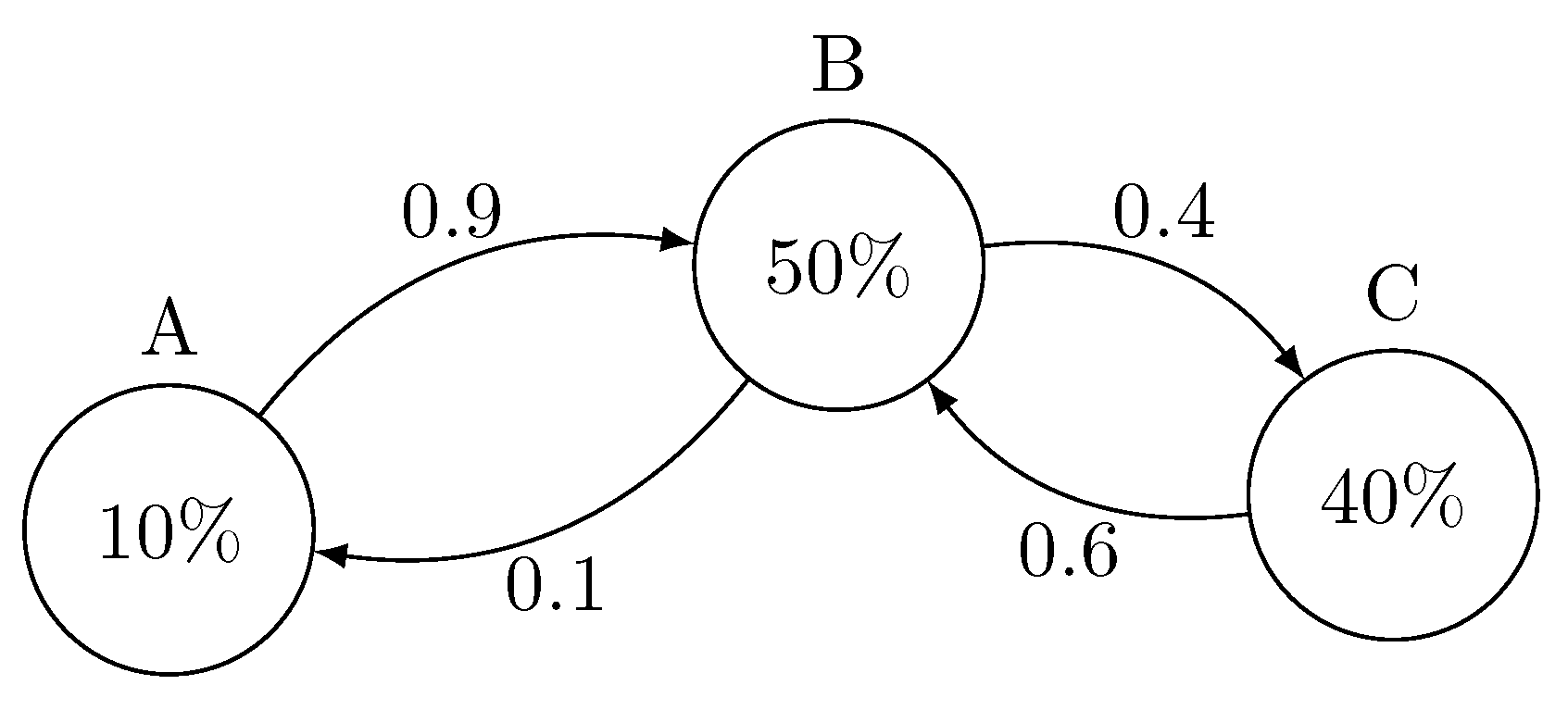
Example 1. 

Suppose there are three zones, namely A, B, and C, characterized by the following consumption percentage: 10%, 50%, and 40%, respectively. This information allows us to deduce the conventional flow among the zones, as shown in Figure 1.

Accepting 100 [MWh] in zone A, 10 [MWh] will be actually used by A, whereas the remaining 90 [MWh] will be sent towards B and C. In particular, B will receive 90 [MWh] (and use 50 [MWh]), and C will receive 40 [MWh]. This way, when a quantity of energy enters the grid through a particular zone, it creates a flow in the entire network.

Another situation is presented. If 60 [MWh] are accepted in zone A and 40 [MWh] in zone B, the energy flow will be the following:

• A uses 10 [MWh], the remaining 50 [MWh] go to B
• B receives 50 [MWh] from A, for a total of 90 [MWh]; 50 [MWh] are used and the remaining 40 [MWh] are moved to C
• C uses the 40 [MWh] coming from B.

To solve the problem automatically, it is better to consider one constraint at a time, splitting the graph into the two macro zones involved.

• Edge AB (Figure 2):
  A moves 90% of the production towards B;
  B and C move 10% of the production towards A

  $$\begin{array}{c}\hfill 0.9\end{array}·60\left[\mathit{MWh}\right]\begin{array}{c}\hfill - 0.1\end{array}·(40+0)\left[\mathit{MWh}\right]=50\left[\mathit{MWh}\right]$$
  actually, moving from A to B.
• Edge BC (Figure 3):
  A and B move 40% of the production towards C;
  C moves 60% of the production towards B

  $$\begin{array}{c}\hfill 0.4\end{array}·(60+40)\left[\mathit{MWh}\right]-0.6·0\left[\mathit{MWh}\right]=40\left[\mathit{MWh}\right]$$
  actually moving from B to C.

The first step in generalizing this procedure is to define the adjacency matrix that characterizes the topology of the Italian energy zones. Figure 4 shows the graph of the Italian energy network, and

Table 1. Adjacency matrix of the graph.

	NORD	CNOR	CSUD	SUD	ROSS	SICI	SARD
NORD	0	1	0	0	0	0	0
CNOR	1	0	1	0	0	0	0
CSUD	0	1	0	1	0	0	1
SUD	0	0	1	0	1	0	0
ROSS	0	0	0	1	0	1	0
SICI	0	0	0	0	1	0	0
SARD	0	0	1	0	0	0	0

is the corresponding adjacency matrix.

Next, the percentage of monthly consumption for each zone is computed using data from the previous year provided by Terna at the download center: https://www.terna.it/it/sistema-elettrico/transparency-report/download-center (accessed on 17 April 2023). Then, the conventional flow coefficients are estimated separately for peak and off-peak periods. This algorithm generalizes the procedure described in the example:

• Every zone i is visited only once;
• For every neighboring zone j, consider the two macro zones I and J resulting from cutting the graph between i and j;
• The coefficient of conventional flow from i to j, denoted by ${\phi }_{ij}$, correspond the consumption percentage of the macro zone J; vice versa, the conventional flow from j to i, i.e., ${\phi }_{ji}$, is the consumption percentage of the macro zone I;
• When a quantity is accepted in a zone, it is important to ensure that it does not cause congestion on the paths that connect the zone to other parts of the network. In particular, when a quantity is accepted in zone k, it has an impact on the arch $(i,j)$: the magnitude of the impact is given by ${\phi }_{ij}$ times the accepted quantity; whereas the sign of the contribution is positive if $k\in I$ (thus the flow takes place from i to j), negative if $k\in J$;
• In other words, let ${\phi }_{ij}^k$ denote the signed conventional flow coefficient, where the sign is determined by k belonging to I or J.

The result is a matrix containing all the signed conventional flow coefficients. For each oriented edge $(i,j)$, there are two constraints:

$$\begin{array}{cc}\hfill \left(\text{off-peak}\right)& \sum _{k=1}^N\sum _{h=1}^{n_k}{\phi }_{ij}^k{x}_h^k\le {\tau }_{ij}\hfill \end{array}$$

(6)

$$\begin{array}{cc}\hfill \left(\mathrm{peak}\right)& \sum _{k=1}^N\sum _{h=1}^{n_k}{\tilde{\phi }}_{ij}^k{x}_h^k+\sum _{k=1}^N\sum _{h=1}^{{\tilde{n}}_k}{\tilde{\phi }}_{ij}^k{\tilde{x}}_h^k\le {\tilde{\tau }}_{ij},\hfill \end{array}$$

(7)

where ${\tau }_{ij}$ and ${\tilde{\tau }}_{ij}$ are the maximum limit values for off-peak and peak time zone from i to j. This information is provided by Terna directly to the participants. The corresponding rows of the matrix A are

$$\begin{array}{cc}\hfill \mathrm{constraint}& (i,j)\text{off-peak:}\hfill \\ \hfill & (\underset{n_1}{\underbrace{{\phi }_{ij}^1,\dots ,{\phi }_{ij}^1}},\dots \dots ,\underset{n_N}{\underbrace{{\phi }_{ij}^N,\dots ,{\phi }_{ij}^N}},\underset{{\tilde{n}}_1}{\underbrace{0,\dots ,0}},\dots \dots ,\underset{{\tilde{n}}_N}{\underbrace{0,\dots ,0}})\hfill \\ \hfill \mathrm{constraint}& (i,j)\mathrm{peak}:\hfill \\ \hfill & (\underset{n_1}{\underbrace{{\tilde{\phi }}_{ij}^1,\dots ,{\tilde{\phi }}_{ij}^1}},\dots \dots ,\underset{n_N}{\underbrace{{\tilde{\phi }}_{ij}^N,\dots ,{\tilde{\phi }}_{ij}^N}}\underset{{\tilde{n}}_1}{\underbrace{{\tilde{\phi }}_{ij}^1,\dots ,{\tilde{\phi }}_{ij}^1}},\dots \dots ,\underset{{\tilde{n}}_N}{\underbrace{{\tilde{\phi }}_{ij}^N,\dots ,{\tilde{\phi }}_{ij}^N}}),\hfill \end{array}$$

while the corresponding entries of the vector $\mathbf{b}$ contain the values ${\tau }_{i,j}$ and ${\tilde{\tau }}_{i,j}$, respectively.

Finally, the number of transmission constraints can be computed. Every oriented edge $(i,j)$ corresponds to two constraints (for peak and off-peak market type). Therefore, the number of transmission constraints is twice the number of oriented edges in the graph of the Italian energy market, namely $2M$. With the number of constraints, it is possible to write down the dimensions of the objects at hand:

$$\begin{array}{cc}\hfill & A\in {\mathbb{R}}^{2M\times D},\hfill \\ \hfill & \mathbf{x},\mathbf{p}\in {\mathbb{R}}^D,\hfill \\ \hfill & \mathbf{b}\in {\mathbb{R}}^{2M}.\hfill \end{array}$$

3.2. Objective Function

Now that all the constraints have been implemented, the objective function needs to be defined: the aim is to maximize the total revenue that results from the offered price multiplied by the corresponding accepted quantity over the accepted quantity of energy. The quantities offered on the peak market are multiplied by a factor $\beta$, which is the proportion of peak hours with respect to the whole period under consideration. According to the guidelines provided by Terna, peak hours are 8:00–19:59, Monday–Friday. This results in the following maximization problem

$$\underset{\mathbf{x}}{max}\left[\sum _{i=1}^N\sum _{j=1}^{n_i}{p}_j^i{x}_j^i+\beta \sum _{i=1}^N\sum _{j=1}^{{\tilde{n}}_i}{\tilde{p}}_j^i{\tilde{x}}_j^i\right],$$

that can be rewritten in the usual form of a scalar product by multiplying the last $\tilde{d}$ components of $\mathbf{p}$ by $\beta$. This reads as

$$\underset{\mathbf{x}}{max}{\left(B\mathbf{p}\right)}^t\mathbf{x},$$

where

$$B=\left(\begin{array}{ll}{I}_d& 0\\ 0& \beta I_d\end{array}\right)\in {\mathbb{R}}^{D\times D}.$$

4. Simulation

The implementation of the model consists in properly defining the variables, as extensively described in the previous section. The programming language R and the Rsymphony library were used, the latter including the function Rsymphony_solve_LP, which allowed for the computation of the optimal variable, i.e., the accepted quantities.

The arguments of the solver Rsymphony_solve_LP are: the vector of objective coefficients $\mathbf{p}$; the matrix of the constraint coefficients A; the character vector with the directions of the constraints, that is “≤”; the vector $\mathbf{b}$ on the right-hand side of the constraints; the list containing the bounds of objective variables, i.e., the vector $\mathbf{0}$ for the lower bounds and $\mathbf{q}$ for the upper bounds; a character vector giving the types of objective variables, which can be continuous, integer, or binary; a logical giving the direction of the optimization.

This solver, however, cannot solve problems where the auction is of the all-or-nothing type: the type “continuous” (resp. “integer”) is chosen, and the decision variables can take any continuous (resp. integer) value between 0 and the offered quantity; on the other hand, if the type “binary” is chosen, the decision variable can only be either 0 or 1.

Consequently, the problem needs to be transformed to ensure that the solver is compatible with the all-or-nothing auction type. The idea is to convert each component $x_j^i\in \{0,{\tilde{q}}_j^i\}$ (resp. ${\tilde{x}}_j^i\in \{0,{\tilde{q}}_j^i\}$) into a binary variable $y_j^i\in \{0,1\}$ (resp. ${\tilde{y}}_j^i\in \{0,1\}$) by dividing by the corresponding offered quantity $q_j^i$ (resp. ${\tilde{q}}_j^i$).

The new decision variable becomes

$$\mathbf{y}=(y_1^1,\dots ,y_{n_1}^1,y_1^2,\dots ,y_{n_2}^2,\dots \dots ,y_1^N,\dots ,y_{n_N}^N,{\tilde{y}}_1^1,\dots ,{\tilde{y}}_{{\tilde{n}}_1}^1,{\tilde{y}}_1^2,\dots ,{\tilde{y}}_{{\tilde{n}}_2}^2,\dots \dots ,{\tilde{y}}_1^N,\dots ,{\tilde{y}}_{{\tilde{n}}_N}^N),$$

where

$$\begin{array}{cc}\hfill & y_j^i:=\frac{x_j^i}{q_j^i},j=1,\dots ,n_i,i=1,\dots ,N,\hfill \\ \hfill & {\tilde{y}}_j^i:=\frac{{\tilde{x}}_j^i}{{\tilde{q}}_j^i},j=1,\dots ,{\tilde{n}}_i,i=1,\dots ,N.\hfill \end{array}$$

The objective function accordingly becomes:

$$\begin{array}{cc}\hfill & \underset{\mathbf{x}}{max}\left[\sum _{i=1}^N\sum _{j=1}^{n_i}{p}_j^i{x}_j^i+\beta \sum _{i=1}^N\sum _{j=1}^{{\tilde{n}}_i}{\tilde{p}}_j^i{\tilde{x}}_j^i\right]\hfill \\ \hfill & \underset{\mathbf{x}}{max}\left[\sum _{i=1}^N\sum _{j=1}^{n_i}{p}_j^i{q}_j^i\frac{x_j^i}{q_j^i}+\beta \sum _{i=1}^N\sum _{j=1}^{{\tilde{n}}_i}{\tilde{p}}_j^i{\tilde{q}}_j^i\frac{{\tilde{x}}_j^i}{{\tilde{q}}_j^i}\right]\hfill \\ \hfill & \underset{\mathbf{y}}{max}\left[\sum _{i=1}^N\sum _{j=1}^{n_i}\left(p_j^i{q}_j^i\right)y_j^i+\beta \sum _{i=1}^N\sum _{j=1}^{{\tilde{n}}_i}\left({\tilde{p}}_j^i{\tilde{q}}_j^i\right){\tilde{y}}_j^i\right].\hfill \end{array}$$

(8)

The resulting vector of objective coefficients is given by the component-wise multiplication of $\mathbf{p}$ and $\mathbf{q}$, namely

$$\hat{\mathbf{p}}=(p_1^1{q}_1^1,\dots ,p_{n_1}^1{q}_{n_1}^1,\dots ,p_1^N{q}_1^N,\dots ,p_{n_N}^N{q}_{n_N}^N,{\tilde{p}}_1^1{\tilde{q}}_1^1,\dots ,{\tilde{p}}_{{\tilde{n}}_1}^1{\tilde{q}}_{{\tilde{n}}_1}^1,\dots ,{\tilde{p}}_1^N{\tilde{q}}_1^N,\dots ,{\tilde{p}}_{{\tilde{n}}_N}^N{\tilde{q}}_{{\tilde{n}}_N}^N).$$

The constraint Equations (6) and (7) also change into

$$\begin{array}{cc}\hfill \left(\text{off-peak}\right)& \sum _{k=1}^N\sum _{h=1}^{n_k}\left({\phi }_{ij}^k{q}_h^k\right)y_h^k\le {\tau }_{ij}\hfill \end{array}$$

(9)

$$\begin{array}{cc}\hfill \left(\mathrm{peak}\right)& \sum _{k=1}^N\sum _{h=1}^{n_k}\left({\tilde{\phi }}_{ij}^k{q}_h^k\right)y_h^k+\sum _{k=1}^N\sum _{h=1}^{{\tilde{n}}_k}\left({\tilde{\phi }}_{ij}^k{\tilde{q}}_h^k\right){\tilde{y}}_h^k\le {\tilde{\tau }}_{ij},\hfill \end{array}$$

(10)

and the corresponding rows of the new matrix $\hat{A}$ are obtained by component-wise multiplying the rows of A by $\mathbf{q}$. The vector $\mathbf{b}$ remains unchanged.

Summing up, the initial problem has been translated into an equivalent problem where the decision variable is binary:

$$\begin{array}{cc}\mathrm{find}\mathrm{a}\mathrm{vector}\hfill & \mathbf{y}\hfill \\ \mathrm{that}\mathrm{maximizes}\hfill & {\left(B\hat{\mathbf{p}}\right)}^t\mathbf{y}\hfill \\ \mathrm{subject}\mathrm{to}\hfill & \hat{A}\mathbf{y}\le \mathbf{b}\hfill \\ \mathrm{and}\hfill & \mathbf{y}\in {\mathbb{Z}}_2^D.\hfill \end{array}$$

(11)

Once $\mathbf{y}$ has been found, $\mathbf{x}$ is recovered by the component-wise multiplication of $\mathbf{y}$ and $\mathbf{q}$.

The model was evaluated for each month of 2019 to test its performance over an entire year. The bidding data are accessible on the Terna website https://www.terna.it/it/sistema-elettrico/mercato-elettrico/ccc (accessed on 22 April 2023). The consumption data of 2018 used to estimate the conventional flow coefficients are also available on Terna’s download center https://www.terna.it/it/sistema-elettrico/transparency-report/download-center (accessed on 22 April 2023).

The simulation results are presented in Figure 5 and Figure 6. The Mean Absolute Percentage Error (MAPE) has been computed, which is shown in

Table 2. MAPE (%) of the prediction of accepted quantities for 2019 (Off-peak market). Green shades correspond to low error, red shades correspond to high error.

	CNOR	CSUD	NORD	ROSS	SARD	SICI	SUD	Mean
January	9.68	0.34	9.18	53.75	5.43			15.68
February	10.18	13.68	0.11	1.81		4.80		6.12
March	3.03	8.54	4.51	0.87	1.76			3.74
April	20.52		6.23		56.54	7.81		18.22
May	1.72		0.24	21.68			4.68	4.05
June		1.48			0.94			0.61
July	3.85		1.12		20.27			4.21
August		0.42	0.00	14.29	1.11			3.95
September	0.00	0.23	0.00	0.00	22.73	8.01		5.16
October	2.55	3.10	5.21	0.00	2.54			2.68
November	3.17	9.15	1.92	20.19	46.89	3.89		17.54
December	0.00	4.29	1.76	5.13	0.00	1.06		2.04
Mean	4.97	3.75	2.52	10.70	14.38	6.51	4.68	7.00

and

Table 3. MAPE (%) of the prediction of accepted quantities for 2019 (Peak market). Green shades correspond to low error, red shades correspond to high error.

	CNOR	CSUD	NORD	ROSS	SARD	SICI	SUD	Mean
January	0.53							0.53
February	0.00	0.10	0.00					0.003
March	1.04	0.89						0.97
April	0.00	0.00	0.00					0.00
May	12.64	33.33	0.79	0.00				11.69
June	0.65	0.00	4.11					1.59
July	0.00	0.00	2.73	0.00				0.68
August	6.31	81.97	7.69	5.95				25.48
September	0.10	0.00	1.88					0.66
October
November	1.49	3.27						2.38
December	2.23	58.47	7.61					22.77
Mean	2.27	17.8	3.1	1.98				6.07

. Extremely high error values (such as in the SUD zone in March) have been excluded, as some other market dynamics unrelated to the model have occurred. Overall the model is able to predict with pretty good precision the quantity allocated in each zone for both the off-peak and peak market. The MAPE below 10% on average confirms this fact.

All the constraints have been satisfied. In addition, it is possible to obtain the saturation level of each transit constraint by computing the quantities on the left-hand side of (9) and (10): the condition being met with equality implies that saturation is reached. Figure 7 shows the saturation level of the transit constraints for the off-peak and peak market during the bid of December 2019.

Finally, the algorithm identifies the assigned quantities for each zone by selecting the submitted bids starting from the highest-priced offers. For each zone, the last accepted bid determines the marginal price of the zone, representing the allocation price for all accepted bids. Figure 8 and Figure 9 compare the predicted and the real marginal prices. Except for some outliers, due to unknown market dynamics unrelated to the model, the predictions are really close to the real values.

5. Conclusions

The allocation of hedging instruments, such as FTRs, plays a critical role in managing the financial risk associated with transmission congestion. By using these instruments, market participants can mitigate their exposure to fluctuations in the price of transmission capacity, which can have a significant impact on their profitability.

This paper presented an LP model that simulates the allocation process of FTRs, taking into account the transit limitations of the electric network as well as the all-or-nothing type of bidding procedure.

Numerical simulations showed good results, with an overall MAPE of approximately 7%, indicating that the model was able to accurately predict the allocation of transmission rights across the network. Additionally, the model was found to be particularly useful for simulating the bidding and allocation procedure, providing participants with an indication of whether their bids were likely to be accepted or not.

A limitation of the proposed model lies in the estimation of coefficients for conventional flow, which is based on the monthly consumption of the previous year; this can potentially result in a loss of accuracy.

Overall, the model represents a significant contribution to the field of energy economics and has the potential to improve the efficiency and effectiveness of the transmission rights allocation process.

References

- Di Persio, L.; Cecchin, A.; Cordoni, F. Novel Approaches to the Energy Load Unbalance Forecasting in the Italian Electricity Market. J. Math. Ind. 2017, 7, 5. [Google Scholar] [CrossRef]
- Rancilio, G.; Bovera, F.; Merlo, M. Revenue Stacking for BESS: Fast Frequency Regulation and Balancing Market Participation in Italy. Int. Trans. Electr. Energy Syst. 2022, 2022, 1894003. [Google Scholar] [CrossRef]
- Panda, M.; Nayak, Y.K. Impact analysis of renewable energy Distributed Generation in deregulated electricity markets: A context of Transmission Congestion Problem. Energy 2022, 254, 124403. [Google Scholar]
- Yusoff, N.I.; Zin, A.A.M.; Khairuddin, A.B. Congestion management in power system: A review. In Proceedings of the 2017 3rd International Conference on Power Generation Systems and Renewable Energy Technologies (PGSRET), Johor Bahru, Malaysia, 4–6 April 2017; pp. 22–27. [Google Scholar]
- Pillay, A.; Karthikeyan, S.P.; Kothari, D. Congestion management in power systems–A review. Int. J. Electr. Power Energy Syst. 2015, 70, 83–90. [Google Scholar] [CrossRef]
- Narain, A.; Srivastava, S.; Singh, S. Congestion management approaches in restructured power system: Key issues and challenges. Electr. J. 2020, 33, 106715. [Google Scholar]
- Simoglou, C.K.; Biskas, P.N. Capacity Mechanisms in Europe and the US: A Comparative Analysis and a Real-Life Application for Greece. Energies 2023, 16, 982. [Google Scholar] [CrossRef]
- Hogan, W.W. Contract networks for electric power transmission. J. Regul. Econ. 1992, 4, 211–242. [Google Scholar] [CrossRef]
- Litvinov, E.; Zheng, T.; Rosenwald, G.; Shamsollahi, P. Marginal loss modeling in LMP calculation. IEEE Trans. Power Syst. 2004, 19, 880–888. [Google Scholar] [CrossRef]
- Cheng, X.; Overbye, T.J. An energy reference bus independent LMP decomposition algorithm. IEEE Trans. Power Syst. 2006, 21, 1041–1049. [Google Scholar]
- Conejo, A.J.; Castillo, E.; Mínguez, R.; Milano, F. Locational marginal price sensitivities. IEEE Trans. Power Syst. 2005, 20, 2026–2033. [Google Scholar] [CrossRef]
- Wu, T.; Alaywan, Z.; Papalexopoulos, A.D. Locational marginal price calculations using the distributed-slack power-flow formulation. IEEE Trans. Power Syst. 2005, 20, 1188–1190. [Google Scholar]
- Chen, L.; Suzuki, H.; Wachi, T.; Shimura, Y. Components of nodal prices for electric power systems. IEEE Trans. Power Syst. 2002, 17, 41–49. [Google Scholar]
- Finney, J.D.; Othman, H.A.; Rutz, W.L. Evaluating transmission congestion constraints in system planning. IEEE Trans. Power Syst. 1997, 12, 1143–1150. [Google Scholar]
- Kristiansen, T. Markets for financial transmission rights. Energy Stud. Rev. 2005, 13, 25–74. [Google Scholar]
- Harvey, S.M.; Hogan, W.W.; Pope, S.L. Transmission capacity reservations implemented through a spot market with transmission congestion contracts. Electr. J. 1996, 9, 42–55. [Google Scholar]
- Shahidehpour, M.; Alomoush, M. Restructured Electrical Power Systems: Operation, Trading, and Volatility, 1st ed.; CRC Press: Boca Raton, FL, USA, 2017. [Google Scholar]
- Shahidehpour, M.; Yamin, H.; Li, Z. Market Operations in Electric Power Systems; John Wiley & Sons, Inc.: New York, NY, USA, 2002. [Google Scholar]
- Alomoush, M.; Shahidehpour, S. Fixed transmission rights for zonal congestion management. IEE Proc. Gener. Transm. Distrib. 1999, 146, 471–476. [Google Scholar]
- Sarkar, V.; Khaparde, S.A. A Comprehensive Assessment of the Evolution of Financial Transmission Rights. IEEE Trans. Power Syst. 2008, 23, 1783–1795. [Google Scholar]
- Mosconi, E.M.; Poponi, S.; Silvestri, C. Financial Risk and market Effects for the Congestion Costs of the electricity System in Italy. Int. J. Therm. Environ. Eng. 2015, 10, 113–120. [Google Scholar]
- Alomoush, M.; Shahidehpour, S. Generalized model for fixed transmission rights auction. Electr. Power Syst. Res. 2000, 54, 207–220. [Google Scholar]
- O’Neill, R.P.; Helman, U.; Hobbs, B.F.; Stewart, W.R.; Rothkopf, M.H. A joint energy and transmission rights auction: Proposal and properties. IEEE Trans. Power Syst. 2002, 17, 1058–1067. [Google Scholar]
- Sarkar, V.; Khaparde, S. A robust mathematical framework for managing simultaneous feasibility condition in financial transmission rights auction. In Proceedings of the 2006 IEEE Power Engineering Society General Meeting, Montreal, QC, Canada, 18–22 June 2006. [Google Scholar]
- Schrijver, A. Theory of Linear and Integer Programming; Wiley: Chichester, UK, 1998. [Google Scholar]
- Luenberger, D. Linear and Nonlinear Programming; Addison-Wesley: Columbus, OH, USA, 1984. [Google Scholar]
- Dantzig, G.B.; Thapa, M.N. Solving Simple Linear Programs. In Linear Programming: 1: Introduction; Springer: New York, NY, USA, 1997. [Google Scholar]
- Dantzig, G.B.; Thapa, M.N. Linear Programming: Theory and Extensions; Springer: New York, NY, USA, 2003; Volume 2. [Google Scholar]
- Mansini, R.; Ogryczak, W.; Speranza, M.G. Linear Models for Portfolio Optimization. In Linear and Mixed Integer Programming for Portfolio Optimization; Springer International Publishing: Cham, Switzerland, 2015; pp. 19–45. [Google Scholar]
- Papahristodoulou, C.; Dotzauer, E. Optimal portfolios using linear programming models. J. Oper. Res. Soc. 2004, 55, 1169–1177. [Google Scholar]
- Konno, H.; Yamamoto, R. Integer programming approaches in mean-risk models. Comput. Manag. Sci. 2005, 2, 339. [Google Scholar]
- Daskalaki, S.; Birbas, T.; Housos, E. An integer programming formulation for a case study in university timetabling. Eur. J. Oper. Res. 2004, 153, 117–135. [Google Scholar]
- Gao, C.; Zhang, Z.; Wang, P. Day-Ahead Scheduling Strategy Optimization of Electric–Thermal Integrated Energy System to Improve the Proportion of New Energy. Energies 2023, 16, 3781. [Google Scholar]
- Aasgård, E.K. Hydropower bidding using linearized start-ups. Energies 2017, 10, 1975. [Google Scholar]
- An, J.; Mikhaylov, A.; Jung, S.U. A Linear Programming approach for robust network revenue management in the airline industry. J. Air Transp. Manag. 2021, 91, 101979. [Google Scholar]
- Azimi, M.; Beheshti, R.; Imanzadeh, M.; Nazari, Z. Optimal allocation of human resources by using linear programming in the beverage company. Univers. J. Manag. Soc. Sci. 2013, 3, 48–54. [Google Scholar]
- Zoltowska, I.; Lin, J. Optimal Charging Schedule Planning for Electric Buses Using Aggregated Day-Ahead Auction Bids. Energies 2021, 14, 4727. [Google Scholar]
- Ma, X.; Sun, D.; Rosenwald, G.; Ott, A. Advanced financial transmission rights in the PJM market. In Proceedings of the 2003 IEEE Power Engineering Society General Meeting (IEEE Cat. No.03CH37491), Toronto, ON, Canada, 13–17 July 2003; Volume 2, pp. 1031–1038. [Google Scholar]
- Biskas, P.N.; Ziogos, N.P.; Bakirtzis, A.G. Analysis of a monthly auction for financial transmission rights and flow-gate rights. Electr. Power Syst. Res. 2007, 77, 594–603. [Google Scholar]
- Kalsi, K.; Elbert, S.; Vlachopoulou, M.; Zhou, N.; Huang, Z. Advanced computational methods for security constrained financial Transmission Rights. In Proceedings of the 2012 IEEE Power and Energy Society General Meeting, San Diego, CA, USA, 22–26 July 2012; pp. 1–8, ISSN 1944-9925. [Google Scholar]