Stability Analysis of EKF-Based SOC Observer for Lithium-Ion Battery

Abstract

The state of charge (SOC) plays a critical role in battery management systems. This paper discusses the stability of the nonlinear SOC observer based on the extended Kalman filter. The model characterizing the lithium-ion battery nonlinearity is the basis of the stability analysis. After balancing the accuracy and the complexity of the models, the Thevenin battery model and the logarithmic fitting OCV (open circuit voltage) model are employed. The stability of the SOC observer is theoretically analyzed from two aspects: model parameters and system nonlinearity. Furthermore, the impact of system noises and nonlinear characteristics on the estimation is explored in a numerical way. For the estimation of SOC, the nonlinearity is mainly reflected in the OCV-SOC function. It is found out that the gradient variation of the OCV-SOC curve is not conducive to the estimation, especially when the gradient is small and the voltage noise is large. In order to improve the estimation performance, the role of matrices Q and R as the design parameters of the SOC observer is discussed. The results indicate that the observer is able to exhibit good stability and performance under appropriate settings.

1. Introduction

Lithium-ion batteries (LiBs) are used as power sources in many fields, especially in electric vehicles, thanks to their favorable performance in energy density, cycle-life and energy efficiency. To ensure the safety of the battery and prolong its service life, it is necessary to carry out detailed and comprehensive management of the battery. The state estimation is the foundation of the battery management system (BMS). The states of battery can be divided into two categories: One is the states which can be directly measured, such as voltage and current; the other is the states can only be obtained with estimation, such as the state of charge (SOC) and the state of health (SOH). SOC, which indicates the amount of charge remaining in a battery, is the core parameter of battery management. If the SOC is accurate enough, the battery can be used without worrying about overcharging or over-discharging.

However, the external characteristics of LiBs exhibit nonlinear behavior which makes the SOC estimation difficult. The nonlinearity of the battery reflects in two aspects: One is that the influence of the working conditions on the external characteristics of LiBs is nonlinear. On the other hand, the relationships between the battery external characteristics and some internal states of the battery are nonlinear. Because of the one-to-one correspondence between OCV (open circuit voltage) and SOC, it is often used as the basis of the SOC estimation. However, at the same time, its nonlinearity complicates the estimation of the SOC. It is helpful to discuss in depth the influence of nonlinear factors on the SOC estimation to obtain higher accuracy.

There are usually two approaches to improve the accuracy of the SOC estimation. The first one is to establish a more accurate nonlinear model to achieve a better approximation of the battery nonlinear characteristics. Based on the relationship between voltage, internal resistance and SOC, Szumanowski and Chang [1] proposed a universally applicable mathematical model which can accurately represent the battery nonlinearity and can be easily used in practice with a microprocessor. Shi et al. [2] proposed a cloud-based data-driven method which uses the self-supervised transformer neural network to model the behavior of a lithium-ion battery cell. Spatiotemporal features were extracted from the field data with an attention-based deep learning approach.

The second strategy is to design a nonlinear algorithm to ensure the accuracy of the SOC estimation. Plett [3] presented an extended Kalman filter (EKF) to combine coulomb counting and electromotive force measurement. Liu et al. used the result of the EKF as the training data for the extreme gradient boosting (XGBoost) model to realize the SOC prediction [4]. Based on the unscented Kalman filter (UKF), a SOC estimation method is proposed in [5].

The objective of this paper is to analyze the influencing mechanism of the system nonlinearity and improve the algorithm performance. EKF is selected as the filtering algorithm, because it often yields powerful and computationally efficient estimators and has been widely employed to determine the SOC.

The convergence of EKF has not rigorously been proven yet. The main difficulty arises from the fact that the EKF equations are only approximate ones. It relies on the first-order linearization to propagate the mean and covariance of the state, then the linearization error comes in inevitably and the Jacobian matrix derivation may be nontrivial. In the last two decades, the study of the convergence properties of EKF has mainly evolved into three different directions.

The first common method is to analyze the long-time behavior of the estimation error between the filter estimate and the partial observation. To bypass the fluctuations of signal noise and observation disturbance, a deterministic state observer is designed as the asymptotic limit of the EKF when the observation and sensor noises tend to zero. Song and Grizzle [6] proved that EKF is a quasi-local asymptotic observer for the discrete nonlinear system with no input, and they gave the observability analysis of the nonlinear system. Moreover, if the system satisfies the observability and controllability conditions, the maximal and the minimal eigenvalues of the solution of the Riccati equation in the algorithm can be determined [7].

The second and more complicated approach is based on the contraction theory, which is developed by Lohmiller and Slotine [8,9]. The main idea of this method is to construct a quadratic form with the inverse of the solution of the Riccati equation, then quantify the estimation error between a couple of close EKF trajectories, thereby limiting the error to a given region. This method takes a partial observation as a deterministic system and requires the filter to be activated in the domain of attraction of the true state. It can be proved that under appropriate observability and controllability conditions, if the corresponding quadratic form is sufficiently regular, the EKF observer can converge locally and exponentially to the true state.

The third strategy is to use the Lyapunov method to ensure the random stability of the EKF algorithm by designing the energy function, which is expressed in terms of the inverse of the Riccati equation. Boutayeb et al. [10] presented a convergence analysis of EKF for deterministic discrete-time nonlinear systems with multiple inputs and outputs, by demonstrating that the candidate Lyapunov function was decreasing without any approximation. Moreover, Reif made a significant contribution to the stability analysis of EKF. Reif et al. used the Lyapunov’s direct method to prove that the EKF observer satisfies the exponential boundedness by introducing the instability coefficient to characterize the stability of the algorithm [11]. In 1999, Reif et al. [12] made a detailed analysis of the error behavior for the discrete EKF. It proved that the estimation error remains bounded if the system satisfies the nonlinear observability rank condition, and if the initial estimation error and the disturbing noise terms are small enough. Then, the stability of the continuous EKF method was analyzed in [13].

This paper focuses on analyzing the stability of the EKF-based SOC observer applied to a nonlinear battery system. The rest of this paper is organized as follows: A description of the fundamental work of the stability analysis is given in Section 2; A stability analysis method of the EKF-based SOC observer is depicted in Section 3; The verification and explanation for the proposed analysis approach is illustrated in Section 4; Finally, the conclusion is presented in Section 5.

2. EKF Stability Analysis Foundations

The stability analysis of the EKF algorithm for the nonlinear battery system is complicated, and some fundamental work needs to be done in advance, including determination of the analytical method and selection of the battery model.

2.1. Algorithm Used in This Study

In the late 1990′s, some influential work was done by Konrad Reif with various co-authors, which advanced the stability analysis of EKF [11, 12, 13]. Combined with the analysis in the previous section, this paper chooses the Lyapunov method for stability analysis. A further explanation on the stability analysis method proposed by Reif et al. is given.

A nonlinear discrete-time system is represented by

$$\left\{\begin{array}{l}{x}_k=f(x_{k-1},u_{k-1})+G_{k-1}{w}_{k-1}\\ y_k=g(x_k,u_k)+D_k{v}_k\end{array}\right.$$

(1)

where $k\in N_0$ is the discrete time, $x_k\in R^q$ is the state, $u_k\in R^p$ is the input, $y_k\in R^m$ is the output, $v_k$, $w_k$ are $R^n$ and $R^l$ valued uncorrelated zero-mean white noise process with identity covariance and $D_k$, $G_k$ are time varying matrices of size $m\times n$ and $q\times l$. The nonlinear maps $f(x_k,u_k)$ and $g(x_k,u_k)$ are assumed to be continuously differentiable with respect to $x_k$.

The discrete-time EKF update process corresponding to the system shown in Equation (1) is as follows:

$$\begin{gathered} {\widehat{x}}_k=f({\widehat{x}}_{k-1},u_{k-1})+K_{k-1}(y_{k-1}-g({\widehat{x}}_{k-1},u_{k-1})) \\ \hspace{1em}\hspace{1em}\hspace{1em}\hspace{1em}\hspace{1em}{P}_k=A_{k-1}{P}_{k-1}{A}_{k-1}^T+Q_{k-1}-K_{k-1}(C_{k-1}{P}_{k-1}{C}_{k-1}^T+R)K_{k-1}^T \\ \hspace{1em}\hspace{1em}\hspace{1em}\hspace{1em}{A}_{k-1}={\left.\frac{\partial f(x_k,u_{k-1})}{\partial x_k}\right|}_{x_k={\widehat{x}}_{k-1}},C_{k-1}={\left.\frac{\partial g(x_k,u_{k-1})}{\partial x_k}\right|}_{x_k={\widehat{x}}_{k-1}} \\ {K}_{k-1}=A_{k-1}{P}_{k-1}{C}_{k-1}^T{[C_{k-1}{P}_{k-1}{C}_{k-1}^T+R_{k-1}]}^{-1} \end{gathered}$$

where R and Q are the instrumental positive definite matrices.

Lemma 1 [12].

If there exists a stochastic process $V({\varsigma }_k)$ as well as real numbers $\underset{\_}{v},\overline{v},u>0$ and $0<\alpha <1$ such that

$$\underset{\_}{v}{‖{\varsigma }_k‖}^2\le V_k({\varsigma }_k)\le \overline{v}{‖{\varsigma }_k‖}^2$$

and

$$E(V_{k+1}({\varsigma }_{k+1})|{\varsigma }_k)-V_k({\varsigma }_k)\le u-\alpha V_k({\varsigma }_k)$$

then the random variable ${\varsigma }_k$ is said to be exponentially bounded in mean square with probability one as

$$E({‖{\varsigma }_k‖}^2)\le \frac{\overline{v}}{\underset{\_}{v}}E({‖{\varsigma }_0‖}^2){(1-\alpha )}^n+\frac{u}{\underset{\_}{v}\alpha }$$

Lemma 1 provides a method to determine the exponential boundedness of a random sequence process. As long as certain conditions are satisfied, the lemma can be used to prove that the estimation error is exponentially bounded.

The detailed analysis is as follows [12]:

First, Equation (1) can be expanded as

$$f(x_k,u_k)-f({\widehat{x}}_k,u_k)=A_k(x_k-{\widehat{x}}_k)+\phi (x_k,{\widehat{x}}_k,u_k)$$

(2)

$$g(x_k)-g({\widehat{x}}_k)=C_k(x_k-{\widehat{x}}_k)+\chi (x_k,{\widehat{x}}_k)$$

(3)

where $\phi (x_k,{\widehat{x}}_k,u_k)$ and $\chi (x_k,{\widehat{x}}_k)$ are the first-order linearized residues.

The estimation error is defined by $e_k=x_k-{\widehat{x}}_k$. Then Equations (2) and (3) yield:

$$\begin{array}{l}{e}_{k+1}=x_{k+1}-{\widehat{x}}_{k+1}=f(x_k,u_k)+G_k{w}_k-[f({\widehat{x}}_k,u_k)+K_k(y_k-g({\widehat{x}}_k))]\\ =(A_k-K_k{C}_k)(x_k-{\widehat{x}}_k)+r_k+s_k\end{array}$$

(4)

where $r_k=\phi (x_k,{\widehat{x}}_k,u_k)-K_k\chi (x_k,{\widehat{x}}_k)$, $s_k=G_k{w}_k-K_k{D}_k{v}_k$.

A Lyapunov function $V_k(e_k)$ is chosen as follows:

$$\begin{array}{l}{V}_{k+1}(e_{k+1})=e_{k+1}^T{P}_{k+1}^{-1}{e}_{k+1}\\ \begin{array}{cc}& \end{array}={(}^{x_k-{\widehat{x}}_k)T}{(}^{A_k-K_k{C}_k)T}{P}_{k+1}^{-1}(A_k-K_k{C}_k)(x_k-{\widehat{x}}_k)\\ \begin{array}{cc}& \end{array}+r_{{}_k}^T{P}_{k+1}^{-1}[2(A_k-K_k{C}_k)e_k+r_k]+s_k^T{P}_{k+1}^{-1}{s}_k\end{array}$$

(5)

Equation (5) yields:

$$\begin{array}{l}E[V_{k+1}(e_{k+1})|e_k]=E[e_k^T{(}^{A_k-K_k{C}_k)T}{P}_{k+1}^{-1}(A_k-K_k{C}_k)e_k|e_k]\\ \hspace{1em}\hspace{1em}\hspace{1em}+E[r_k^T{P}_{k+1}^{-1}[2(A_k-K_k{C}_k)e_k+r_k]|e_k]\\ \hspace{1em}\hspace{1em}+E[2s_k^T{P}_{k+1}^{-1}[(A_k-K_k{C}_k)e_k+r_k]]|e_k]+E[s_k^T{P}_{k+1}^{-1}{s}_k|e_k]\end{array}$$

(6)

According to Lemma 1 and considering the nonlinear stochastic system given by Equation (1), let the following assumptions hold:

(a)

For every $k\ge 0$, $A_k$ is nonsingular, and there are real numbers $\overline{a},\overline{c}>0$ such that $‖A_k‖\le \overline{a}$ and $‖C_k‖\le \overline{c}$ are fulfilled (throughout this paper, $‖·‖$ denotes the Euclidian norm of real vectors or the spectral norm of real matrices).

(b)

There are real numbers $\epsilon ,\delta ,\underset{\_}{q},\underset{\_}{r}>0$ such that the following bounds on various matrices are fulfilled: $‖e_0‖\le \delta$, $G_k{G}_k^T\le \epsilon I$, $D_k{D}_k^T\le \epsilon I$, $\underset{\_}{q}I\le Q_k$, $\underset{\_}{r}I\le R_k$.

(c)

The error covariance matrix $P_k$ is bounded via $\underset{\_}{p}I\le P_k\le \overline{p}I$ if there are $\underset{\_}{p},\overline{p}>0$.

(d)

There are positive real numbers ${\epsilon }_{\phi },{\epsilon }_{\chi },{\delta }_{\phi },{\delta }_{\chi }>0$ such that the nonlinear function $\phi$ in Equation (2) and $\chi$ in Equation (3) are bounded via $‖\phi (x_k,{\widehat{x}}_k,u_k)‖\le {\epsilon }_{\phi }{‖x_k-{\widehat{x}}_k‖}^2$, $‖\chi (x_k,{\widehat{x}}_k)‖\le {\epsilon }_{\chi }{‖x_k-{\widehat{x}}_k‖}^2$, with $‖x_k-{\widehat{x}}_k‖\le {\delta }_{\phi }$ and $‖x_k-{\widehat{x}}_k‖\le {\delta }_{\chi }$.

Then the estimation error $e_k$ is exponentially bounded in mean square with probability one.

Under the above assumptions, the following conclusions can be drawn from the system shown in Equation (1):

(a)

The first term on the right-hand side of Equation (6) is bounded via ${(A_k-K_k{C}_k)}^T{P}_{k+1}^{-1}(A_k-K_k{C}_k)\le (1-\alpha )P_k^{-1}$ and there is $1-\alpha ={[1+\frac{\underset{\_}{q}}{\overline{p}{(\overline{a}+\overline{a}\overline{p}{\overline{c}}^2/\underset{\_}{r})}^2}]}^{-1}$. It represents the effect of various coefficient matrices in the recursive process.

(b)

The second term on the right-hand side of Equation (6) is bounded via $r_{{}_k}^T{P}_{k+1}^{-1}[2(A_k-K_k{C}_k)e_k+r_k]\le {\kappa }_{nonl}{‖x_k-{\widehat{x}}_k‖}^3$, with ${\epsilon }^{\prime }={\epsilon }_{\phi }+\overline{a}\overline{p}\overline{c}\frac{1}{\underset{\_}{r}}{\epsilon }_{\chi }$, ${\delta }^{\prime }=\min ({\delta }_{\phi },{\delta }_{\chi })$, ${\kappa }_{nonl}={\epsilon }^{\prime }\frac{1}{\underset{\_}{p}}[2(\overline{a}+\overline{a}\overline{p}{\overline{c}}^2/\underset{\_}{r})+{\epsilon }^{\prime }{\delta }^{\prime }]$. This term represents the effect of model nonlinearity on the error upper bound.

(c)

Since $v_k$ and $w_k$ are uncorrelated, the expectation value of the cross-terms containing both $v_k$ and $w_k$ will vanish. Then, there is $E(s_k^T{P}_{k+1}^{-1}[(A_k-K_k{C}_k)e_k+r_k])=0$.

(d)

The last term is bounded via $E[s_k^T{P}_{k+1}^{-1}{s}_k|e_k]\le {\kappa }_{noise}\epsilon$, with ${\kappa }_{noise}=\frac{q}{\underset{\_}{p}}+\frac{m{\overline{a}}^2{\overline{p}}^2{\overline{c}}^2}{\underset{\_}{p}{\underset{\_}{r}}^2}$.

This item characterizes the influence of model noise on the error.

In summary, the above results yield:

$$E[V_{k+1}(e_{k+1})|e_k]\le (1-\alpha )V_k(e_k)+{\kappa }_{nonl}{‖x_k-{\widehat{x}}_k‖}^3+{\kappa }_{noise}\epsilon$$

then,

$$E[V_{k+1}(e_{k+1})|e_k]-V_k(e_k)\le {\kappa }_{nonl}{‖x_k-{\widehat{x}}_k‖}^3+{\kappa }_{noise}\epsilon -\alpha V_k(e_k)$$

(7)

Equation (7) meets the stability theorem. The detailed proof is in [12].

While Reif et al. proposed the above method, it was pointed out that the method is suitable for systems satisfying the nonlinear observability condition. Furthermore, the initial estimation error and the disturbing noise terms should be small enough. This paper applies the method to the battery system to analyze the stability of the EKF-based SOC observer and focuses on the possibility of establishing the preconditions and the specific requirements for the battery model.

2.2. Battery Model

The battery model is the basis of the algorithm. An accurate model is conducive to capture key behaviors of the battery. The accuracy of the model is closely related to its complexity. It is important to strike a balance between model complexity and accuracy so that the model can be embedded in a microprocessor and provide accurate results in real-time. However, the complex nonlinear chemical reactions of LiB lead to the nonlinear and time-varying characteristics. These characteristics are influenced by many factors, such as anode and cathode materials, environment and charging/discharging rate, which pose great difficulties for battery modeling.

Literatures provide several battery models for SOC estimation, which can be divided into three categories: the electrochemical model, the neural network model and the equivalent circuit model. The electrochemical model is proposed based on the electrochemical theory and is mainly used for the structural optimization and parameter calculation. This type of model is usually complex and time-consuming, and it can hardly simulate the dynamic performance. The accuracy of the neural network model depends on the complexity of neural network and the number of input variables. Different from the two types of models above, the equivalent circuit model is developed by using resistors, capacitors and voltage sources to form a circuit network. It is widely used for its simplicity and easy handling. Commonly used equivalent circuit models of battery are the Rint model, the Thevenin model [14] and the PNGV model.

When using EKF algorithm in SOC estimation, it is required that the state equation can be written in the differential form. Therefore, considering the computational complexity, this paper selects the Thevenin model for analysis. According to the Kirchhoff’s circuit law, the expression is as follows:

$$\left\{\begin{array}{c}{C}_p\ast {\dot{V}}_{p,t}+\frac{V_{p,t}}{R_p}=I_t\\ \frac{d{V}_{p,t}}{dt}+\frac{V_{p,t}}{C_p\ast R_p}=\frac{1}{C_p}\ast I_t\end{array}\right.$$

(8)

where $C_p$ is the polarization capacitance, $R_p$ is the polarization resistance, V_p,t is the polarization voltage and $I_t$ is the current.

After discretization, the state equation and measurement equation of the system are as follows:

$$\left\{\begin{array}{l}{x}_{k+1}=A_k{x}_k+B_k{i}_k+w_k\\ y_k=h(x_k,u_k)+v_k=V_{OC}-\left[\begin{array}{cc}1& 0\end{array}\right]x_k-i_k{R}_0+v_k\end{array}\right.$$

(9)

where

$$\begin{gathered} x_k=\left[\begin{array}{c}{V}_{p,k}\\ SO{C}_k\end{array}\right] \\ {A}_k=\left[\begin{array}{cc}\mathit{exp}(-\frac{△t}{C_p{R}_p})& 0\\ 0& 1\end{array}\right] \\ {B}_k=\left[\begin{array}{c}{R}_p[1-\mathit{exp}(-\frac{△t}{C_p{R}_p})]\\ -\eta △t/C_a\end{array}\right] \end{gathered}$$

$\eta$ is the Coulomb efficiency, $△t$ is the sampling time, $C_a$ is the battery capacity, $V_{OC}$ is the open circuit voltage, $R_0$ is the battery ohmic resistance, $w_k$ is the current noise, $v_k$ is the voltage noise.

3. EKF-Based SOC Observer Stability Analysis

Since the 1960’s, many research activities have been conducted on the state estimation of nonlinear dynamic systems. In particular, [15] constructed an observer for a system with unknown initial state value, which was quite a challenge. It was pointed out that the observer is actually a limited nonlinear filter. References [16,17] analyzed the asymptotic behavior of the observers for different systems and provided the theoretical basis for the application of the method. Reference [18] designed an EKF-based frequency tracker and explicitly pointed out that EKF is a suboptimal estimator of the state. In the estimator design, the matrices $Q$ and $R$ can no longer be regarded as the noise covariances. It means that the matrices are design parameters of the observer, although the usual implication is that the values should be obtained through system identification.

When using the EKF-based observer to estimate SOC, there are the following concerns: First, the initial value is unknown; Second, due to the limitations of the system modeling methods, model errors are inevitable; Third, the first-order linearization introduces errors into the derivation process. Therefore, it is necessary to analyze the performance of the observer.

3.1. System Parameters Analysis

Among the parameters of the system shown in Equation (9), the coulomb efficiency is usually set to a constant close to 1. The rest of them are obtained through parameter identification. Within a certain range, the ohmic resistance hardly changes with the SOC, and the battery capacity slowly decreases as the battery ages. Therefore, they are set as constants in this paper. For positive polarization capacitance and polarization resistance, the matrix $A_k$ is nonsingular, and $‖A_k‖=1$ with $\exp (-\frac{△t}{C_p*R_p})<1$, which is for the stability condition (a).

In addition to the model parameters mentioned above, $Q$ and $R$ play a central role in the convergence of the EKF observer. In the case of linear stochastic systems, optimal filtering in the maximum likelihood is obtained when $Q$ and $R$ are the covariance matrices of the system noises. The matrices describe the impact of noise terms on the filtering algorithm in the recursive process, and the nature of the filtering algorithm is to distinguish the true state value from the background noises. However, for nonlinear systems, optimality has not been proved. The matrices $Q$ and $R$ need not to be the covariances of the noise terms. Any positive definite matrices can be chosen [12]. Note that inappropriate values may render the algorithm less robust. Thus, it is worth analyzing the role of these two instrumental matrices in the behavior of the EKF observer. Boutayeb et al. [10] presented convergence analysis of EKF used as an observer for nonlinear deterministic discrete-time system. It stated that the matrices $Q$ and $R$ in the observer could be defined according to the actual needs. Based on the above conclusions, combined with the selected battery model, it can be drawn that there are $\underset{\_}{q},\underset{\_}{r}>0$ yielding $\underset{\_}{q}I\le Q$ and $\underset{\_}{r}I\le R$ for the stability condition (b). The relevant discussion of $Q$ and $R$ is proposed in Section 4.

3.2. System Nonlinearity Analysis

For the battery model, in addition to the above several parameters, the most important factor influencing the stability of the algorithm is nonlinearity, which is manifested in the OCV-SOC curve.

The influence of battery nonlinearity on the algorithm is reflected in two aspects: One is the matrix generated through the first-order linearization, the other is the higher-order residual left after the linearization.

In $C_k$, which is

$$C_k={\left.\frac{\partial h}{\partial x}\right|}_{x={\widehat{x}}_{k-1}}=\left[\begin{array}{cc}-1& {\left.\frac{\partial V_{OC}}{\partial SOC}\right|}_{SOC=S\widehat{O}{C}_{k-1}}\end{array}\right],$$

the value of $\frac{\partial V_{OC}}{\partial SOC}$ is closely related to the test data and the fitting model. Under the reasonable definition, there is no case of $\frac{\partial V_{OC}}{\partial SOC}=0$ or infinity at the endpoints in the fitting model. Therefore, there is $\overline{c}>0$ so that $‖C_k‖\le \overline{c}$ holds for the stability condition (a).

In addition, according to the relevant conclusion of observability, the observability matrix of the linearized observation equation is as follows:

$$O_k=\left(\begin{array}{c}{C}_k\\ C_k{A}_k\end{array}\right)=\left(\begin{array}{cc}-1& {\left.\frac{\partial V_{OC}}{\partial SOC}\right|}_{SOC=S\widehat{O}{C}_{k-1}}\\ -\mathit{exp}(-\frac{△t}{C_p\ast R_p})& {\left.\frac{\partial V_{OC}}{\partial SOC}\right|}_{SOC=S\widehat{O}{C}_{k-1}}\end{array}\right)$$

where $\exp (-\frac{△t}{C_p*R_p})<1$ and ${\left.\frac{\partial V_{OC}}{\partial SOC}\right|}_{SO{C}_k=S\widehat{O}{C}_k}\ne 0$. Therefore, it yields $rank(O_k)=2$. So, the selected system is locally weakly observable at every $x_k$ and the open neighborhood of $x_k$. Gauthier and Bornard [19] proved that the single output system is observable if it is locally weakly observable at every $x_k$.

According to the linear system controllability conditions, the controllability matrix can be obtained:

$$M_k=(\begin{array}{cc}{B}_k& A_k{B}_k\end{array})=\left(\begin{array}{cc}{R}_p[1-\mathit{exp}(-\frac{\Delta t}{C_p\ast R_p})]& R_p\ast [1-\mathit{exp}(-\frac{\Delta t}{C_p\ast R_p})]\ast \mathit{exp}(-\frac{\Delta t}{C_p\ast R_p})\\ -\eta \frac{\Delta t}{C_a}& -\eta \frac{\Delta t}{C_a}\end{array}\right)$$

where $\eta \frac{\Delta t}{C_a}\ne 0$. Since $rank(M_k)=2$, the system is controllable.

The system is observable and controllable, and there exist $\underset{\_}{p}=\frac{1}{{\beta }_2+1/{\alpha }_2}$ and $\overline{p}={\alpha }_1+1/{\beta }_1$, so that $\underset{\_}{p}I\le P_k\le \overline{p}I$, where ${\alpha }_1,{\alpha }_2,{\beta }_1,{\beta }_2$ are the coefficients of the controllability and observability inequalities of the system. This is for the stability condition (c).

For the higher-order residual of the measurement equation, there is

$$\chi (x_k,{\widehat{x}}_k)=\frac{1}{2}{(x_k-{\widehat{x}}_k)}^T*D_k*(x_k-{\widehat{x}}_k)+{(x_k-{\widehat{x}}_k)}^T*T*(x_k-{\widehat{x}}_k)$$

where ${\left.D_k=\frac{{\partial }^{2}h}{\partial x^2}\right|}_{x={\widehat{x}}_k}={\left.\left(\begin{array}{cc}0& 0\\ 0& \frac{{\partial }^2{V}_{OC}}{\partial SO{C}^2}\end{array}\right)\right|}_{SOC=S\widehat{O}{C}_k}$ is the Hessian matrix, and ${(x(k)-\widehat{x}(k))}^T*T*(x(k)-\widehat{x}(k))$ is the third-order residual. Using the well-known triangle inequality for norms

$$‖x+y‖\le ‖x‖+‖y‖,$$

yields

$$‖\chi (x_{k,}{\widehat{x}}_k)‖\le \frac{1}{2}\ast ‖D_k‖\ast {‖(x_k-{\widehat{x}}_k)‖}^2+‖T‖\ast {‖(x_k-{\widehat{x}}_k)‖}^2$$

Then there is ${\epsilon }_{\chi }=\frac{1}{2}‖D_k‖+‖T‖$ for the stability condition (d).

4. Numerical Analysis and Algorithm Improvement

There are very few papers on the stability of battery SOC observers. Dey et al. designed two nonlinear SOC observers. The stability of the error dynamics in the presence of model uncertainty was carried out [20]. Lotfi et al. developed a switched SDRE (state-dependent-Riccati-equation) filter for SOC estimation by employing time-dependent-switching estimation error covariance matrix. The estimation error stability analysis helped to determine the switching frequency [21]. This paper focuses on the impact of system nonlinearity and measurement noises coupling, and is based on EKF. EKF is a simpler algorithm that is easier to apply to production vehicles. Meanwhile, because the theoretical tools for nonlinear systems are not sufficient, numerical analysis becomes more important.

4.1. Numerical Simulation and Analysis

A suitable fitting model is needed to apply the measured OCV data to the SOC estimation. The fitting accuracy, the complexity and the computing cost should be considered comprehensively in modeling. Two commonly used models are the polynomial exponential fitting model and the logarithmic fitting model. The former uses the polynomial to fit the OCV-SOC curve. The structure is simple, and there is no need to deal with two endpoints specially. However, with an increase in the polynomial order, the complexity of the model also increases rapidly, but the fitting effect has not improved significantly. The logarithmic fitting model is more conducive to reflect the battery nonlinearity and its fitting accuracy is higher. The main disadvantage of the logarithmic model is that the structure is complex and two endpoints of the interval need to be defined specially.

For the logarithmic fitting model, the observability rank condition is fulfilled at every $x_k$. As for the 6-order polynomial model, the observability matrix is not full rank at some $x_k$. Therefore, this paper chooses the logarithmic fitting model to analyze the error behavior.

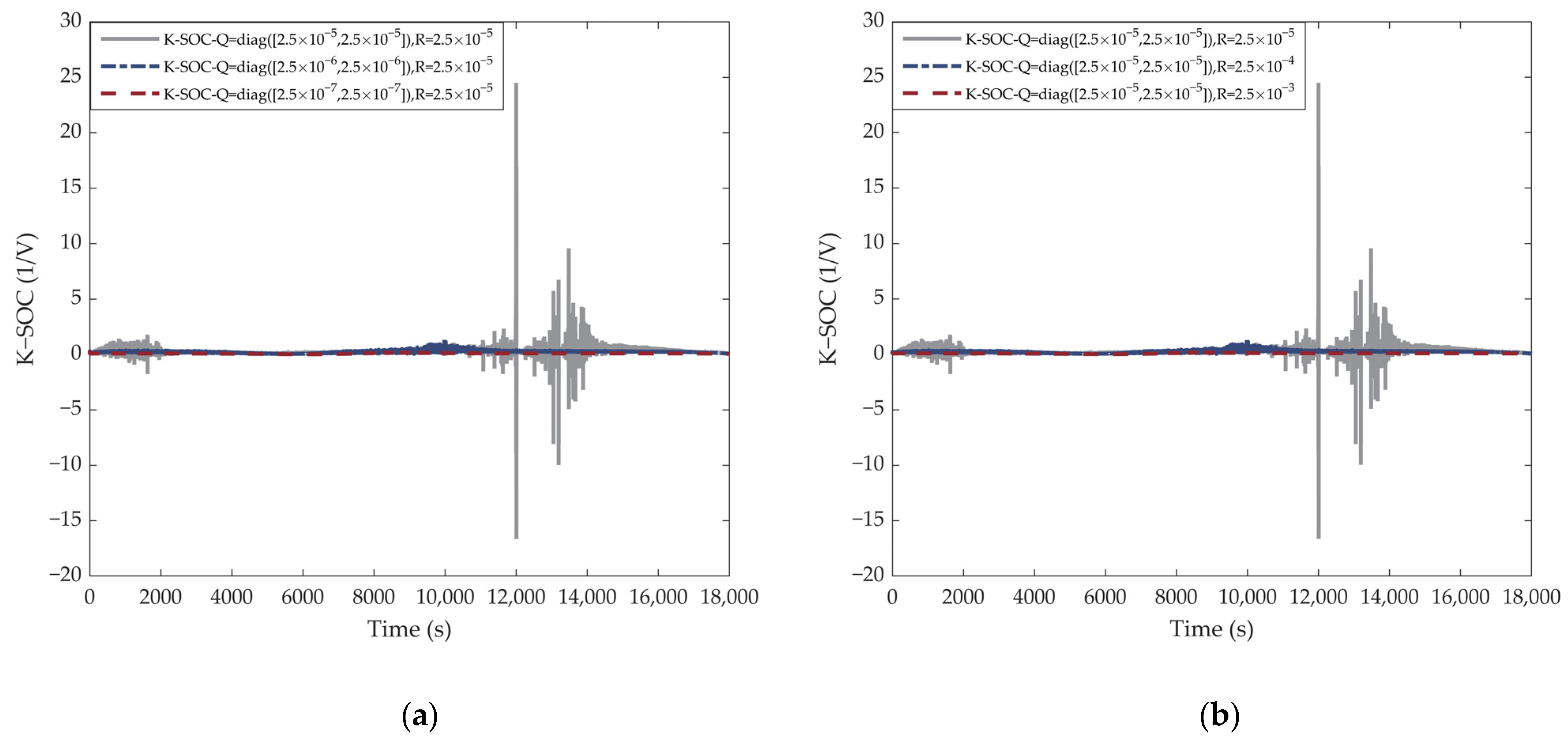
4.1.1. Noise Analysis

Whether the system is linear or nonlinear, noise is inevitable. For the two noises of the system shown in Equation (9), the main role is the voltage noise, and its influence is reflected in the voltage value of the innovation.

$$\begin{array}{l}{x}_{k|k}=x_{k|k-1}+K_k(y_k-h(x_{k|k-1},u_k)) \\ =x_{k|k-1}+K_k\left[h(x_k,u_k)-h(x_{k|k-1},u_k)\right]+K_k{v}_k\end{array}$$

(10)

The last term in the above equation represents the error introduced by the noise. The effect of the voltage noise is significant in the linearization process because the resulting state value is the basis of the Taylor expansion in the next step.

The coefficient matrix $C_k$ obtained through the linearization is affected by the previous state estimate. As a result, the error is passed to the matrix through the state. Because the function $V_{OC}(SOC)$ and its first derivative are nonlinear, the voltage noise further introduces non-additive errors into the linearization process. The inaccurate coefficient matrix in turn affects the update of the state and the error covariance in the next step.

Comparing Figure 1a,b, it shows that, as the voltage noise variance decreases, the estimation effect significantly improves; when the current noise is adjusted similarly, the estimation curves are almost the same. This is consistent with the above theoretical analysis. It is worth noting that the estimation error increases when the OCV-SOC curve enters its plateau. In this case, the measurement equation can be approximated as

$$\begin{array}{l}{y}_k=h(x_k,u_k)+v_k\approx C_k{x}_k-i_k{R}_0+v_k=\left[\begin{array}{cc}-1& c_k\end{array}\right]\left[\begin{array}{l}{V}_{p,k}\\ SO{C}_k\end{array}\right]-i_k{R}_0+v_k\\ \begin{array}{cc}& \end{array}\hspace{1em}=c_{k}SO{C}_k-V_{p,k}-i_k{R}_0+v_k\end{array}$$

(11)

where

$$c_k={\left.\frac{\partial V_{OC}}{\partial SOC}\right|}_{SOC=S\widehat{O}{C}_{k-1}}$$

In Equation (11), $c_k$ is quite small in the plateau of the OCV-SOC curve for the gentle gradient. This makes the updated value of the first three terms in the equation very close to the noise $v_k$, or even smaller. It means that, in this case, it is difficult to distinguish the state from the noise, so the estimation effect is poor. In other words, the impact of the voltage noise on the estimation result is more significant.

After the above analysis, it can be known that the system noise introduces errors in each step of the update procedure. Although these errors are caused by the system noise, they have different characteristics from the original white noise after passing through the state into the system and can no longer be easily eliminated in subsequent iteration steps as in the linear system. This means that the error cannot be compensated in a short period of time, and the new iteration step will introduce the new error which makes the number of the iteration steps closely related to the algorithm performance. Therefore, it is necessary to consider the influence of the sampling step size. In order to highlight the effect of changing the sampling step size under the noise disturbance, matrices Q and R are chosen as the covariance of the process noise and the measurement noise, respectively. On this basis, different sampling steps are set for simulation.

It can be clearly seen from Figure 2 that the algorithm improves with an increase in sampling step size. When the sampling step size is 10 s, the estimation error is small enough, so that the estimation curve almost coincides with the reference one. This is because the number of sample steps decreases with an increase in step size, which reduces the number of introduced errors.

4.1.2. Nonlinearity Analysis

In the practical applications, we want to have a nonlinear theory capable of handling the same broad array of questions as the linear theory. However, in 1982, Casti [22] summed up that seeking a completely general theory of nonlinear systems is a relatively harmless activity full of many pleasant surprises and disappointments, but ultimately unrewarding. Faced with this tricky situation, a compromise approach is making an approximate for the nonlinear system with the linearization technique. Lee and Markus [23] demonstrated that the observability of the linearized system at the equilibrium point and its neighborhood is locally consistent with the observability of the nonlinear system. Wang Xin [24] pointed out that there is an application premise of the linearization for the nonlinear system, that is:

$$A={\left.\frac{\partial f}{\partial x}\right|}_{x^{*}}\ne 0_{n\times n}$$

(12)

According to the qualitative theory of the ordinary differential equation, this means the original system has similar dynamic behavior to the linearized system near the equilibrium point. On the contrary, if the condition is not met, the nonlinear system characteristics cannot be explained by the linear theory, and the linearization analysis method is no longer applicable.

It can be seen from Section 3.1 that the coefficient matrix of the state equation satisfies the linearization condition shown in Equation (12). This lays the foundation for the succeeding analysis using the linear theory. Drawing from the experience of the observability analysis of the nonlinear system, the linear theory of Kalman filter will be applied to analyze the performance of the EKF algorithm of the battery system.

The performance characteristics of the algorithm for a nonlinear system after linearization are determined by the linear Kalman filter. In Kalman filter algorithm, the error covariance indicates the state estimation effect. If the initial conditions and the noise characteristics of the system are not accurately known, the direct relationship between P and the estimation error in the original definition of the Kalman filter is no longer satisfied, P obtained through the algorithm recursion is only the estimated value of the error covariance. In this regard, Yang Xudong et al. [25] established a relation between the estimated value of the error covariance and its true value for the system with inaccurate parameters and proposed the idea of using the estimate of the error covariance to characterize the performance of the Kalman filter approximately.

Consider a simple one-dimensional stationary system,

$$\left\{\begin{array}{l}{x}_k=a{x}_{k-1}+w_{k-1}\\ y_k=c{x}_k+v_k\end{array}\right.$$

(13)

where $w_{k-1}$ and $v_k$ are uncorrelated zero-mean white noise process with identity covariance $Q$ and $R$, respectively. There are $\alpha$, $\beta$, $\lambda >0$, and $\widehat{Q}=\alpha Q$, $\widehat{R}=\beta R$, ${\widehat{P}}_0=\lambda P_0$.

From

Table 1. The relationship between the estimated error covariance and the true value.

For $k=1$:
The estimated value:	The true value:
${\widehat{P}}_{1|0}=a^2{\widehat{P}}_{0|0}+\widehat{Q}=a^2\lambda P_0+\alpha Q$ ${\widehat{K}}_1=\frac{c{\widehat{P}}_{1|0}}{c^2{\widehat{P}}_{1|0}+\widehat{R}}$ ${\widehat{P}}_{1|1}=(1-{\widehat{K}}_{1}c){\widehat{P}}_{1|0}=\frac{\beta R(a^2\lambda P_0+\alpha Q)}{c^2(a^2\lambda P_0+\alpha Q)+\beta R}$	$P_{1|0}=a^2{P}_0+Q$ $K_1=\frac{c{P}_{1|0}}{c^2{P}_{1|0}+R}$ $P_{1|1}=(1-K_{1}c)P_{1|0}=\frac{R(a^2{P}_0+Q)}{c^2(a^2{P}_0+Q)+R}$
The ratio coefficient: ${\eta }_1=\frac{{\widehat{P}}_{1|1}}{P_{1|1}}=\frac{\beta (a^2\lambda P_0+\alpha Q)[c^2(a^2{P}_0+Q)+R]}{[c^2(a^2\lambda P_0+\alpha Q)+\beta R](a^2{P}_0+Q)}$
For $k=2,3,4,\dots$:
The estimated value:	The true value:
${\widehat{P}}_{k+1|k}=a^2{\widehat{P}}_{k|k}+\widehat{Q}=a^2{\eta }_k{P}_{k|k}+\alpha Q$ ${\widehat{K}}_{k+1}=\frac{c{\widehat{P}}_{k+1|k}}{c^2{\widehat{P}}_{k+1|k}+\widehat{R}}$ ${\widehat{P}}_{k+1|k+1}=(1-{\widehat{K}}_{k+1}c){\widehat{P}}_{k+1|k}=\frac{\beta R(a^2{\eta }_k{P}_{k|k}+\alpha Q)}{c^2(a^2{\eta }_k{P}_{k|k}+\alpha Q)+\beta R}$	$P_{k+1|k}=a^2{P}_{k|k}+Q$ $K_{k+1}=\frac{c{P}_{k+1|k}}{c^2{P}_{k+1|k}+R}$ $P_{k+1|k+1}=(1-K_{k+1}c)P_{k+1|k}=\frac{R(a^2{P}_{k|k}+Q)}{c^2(a^2{P}_{k|k}{}_0+Q)+R}$
The ratio coefficient: ${\eta }_{k+1}=\frac{{\widehat{P}}_{k+1|k+1}}{P_{k+1|k+1}}=\frac{\beta (a^2{\eta }_k{P}_{k|k}+\alpha Q)[c^2(a^2{P}_{k|k}+Q)+R]}{[c^2(a^2{\eta }_k{P}_{k|k}+\alpha Q)+\beta R](a^2{P}_{k|k}+Q)}$

The “ ^ “ symbol indicates the estimated value of the system.

, it can be concluded that there is a proportional relationship between the estimated value and the true value of the error covariance. Therefore, the estimate can be used to describe the performance of the algorithm approximately.

Based on further analysis of the characteristics of error covariance estimation, a steady-state Kalman filter method is proved and applied [26], as described below.

For a linear stationary system, which is completely controllable and fully observable, if the initial value of the estimated error covariance matrix $P$ is an arbitrary symmetric non-negative matrix and $P_{1|0}\ge 0$ holds, there is always an upper limit of the Riccati matrix equation in the Kalman filter algorithm (cf., [27]):

$$\underset{k\to \infty }{\lim }{P}_{k+1|k}=\Sigma$$

(14)

where the upper limit $\Sigma$ is the solution of the steady-state matrix Riccati equation:

$$\Sigma =A[\Sigma -\Sigma C^T{(C\Sigma C^T+R)}^{-1}C\Sigma ]A^T+Q$$

(15)

It should be noted that the limit $\Sigma$ is independent of the initial value $P_0$ of the estimation error covariance matrix. Meanwhile, there are limits:

$$\begin{gathered} \underset{k\to \infty }{\lim }{P}_{k|k}=\overline{P} \\ \underset{k\to \infty }{\lim }{K}_k=\overline{K} \end{gathered}$$

According to the five-step iterative procedures of the Kalman filter, there is a relationship among these three limits:

$$\begin{array}{l}\Sigma =A\overline{P}{A}^T+Q\\ \overline{K}=\Sigma C^T{\left(C\Sigma C^T+R\right)}^{-1}\\ \overline{P}=\left[I_n-\overline{K}C\right]\Sigma \end{array}$$

This means that there is a limit for the estimation accuracy. The limit is determined by the variance of the process noise and the measurement noise.

Equation (16) is obtained through mathematical derivation.

$$\overline{P}=\frac{2}{\sqrt{\frac{4a^2{c}^2}{QR}+{\left[\frac{c^2}{R}+\left(\frac{1-a^2}{Q}\right)\right]}^2}+\frac{c^2}{R}+\left(\frac{1-a^2}{Q}\right)}$$

(16)

From Equation (16), it can be concluded that the stable value $\overline{P}$ of the estimation error covariance is determined by the system parameters.

In order to obtain the relationship between the limit $\overline{P}$ and the parameter matrix $C_k$ of the Thevenin model, which is a two-dimensional system, preliminary verification is performed using linear OCV-SOC curves which are artificially set to different slopes. Corresponding to these OCV-SOC curves, the curves of the element corresponding to the SOC in the estimation error covariance matrix are shown in Figure 3. It can be seen from Figure 3 that, for the Thevenin model, the element corresponding to the SOC in the estimation error covariance matrix also has a stable value, and the stable value increases as the slope of the OCV-SOC curve $c_k$ decreases. Furthermore, the smaller $c_k$ is, the more sensitive $\overline{P}$ is to $c_k$. This phenomenon can be confirmed from Equation (16), where $c$ is in the form of a square in the denominator. It is obvious that the change rate of $\overline{P}$ is more dramatic when $c_k$ is close to 0.

EKF is equivalent to linearizing a nonlinear model into linear constant coefficient equations at step $k$ and its neighborhood. Using the result of the previous step as the initial condition of step $k$, Kalman filtering is applied to the update process. Therefore, like the observability analysis method of nonlinear systems (cf., [24]), the above conclusion of linear system can be applied. The performance of EKF is also characterized by the estimate of the error covariance. The error covariance estimate also has a stable value, and the stable value at step $k$ is defined as ${\overline{P}}_k$, which represents the ability to constrain the error covariance estimate $P_k$.

The OCV curve obtained through logarithmic fitting shown in Figure 4a is used for the simulation of discharge. As can be seen from Figure 4b, the estimation error of SOC varies as the discharge progresses. The error of the beginning and the end of the discharge is quite small, while a large estimation error occurs in the middle stage. The reason for this phenomenon is the difference in the error covariance estimate $P_k$ in these three stages shown in Figure 4c caused by the change of $c_k$, which is the element corresponding to SOC in the coefficient matrix $C_k$ shown in Figure 4d. At the beginning of the discharge, according to the above analysis, the large $c_k$ gets a small stable value ${\overline{P}}_k$ which constrains $P_k$ in the actual update process. Therefore, the SOC estimate can overcome the influence of the initial value error and approach the reference value. Then, as $c_k$ decreases, the stable value ${\overline{P}}_k$ increases continuously, which makes the error covariance estimate $P_k$ also increase continuously without a chance to reach the stable value, and the estimation curve gradually deviates from the reference one. $c_k$ continues to decrease until it enters the flat section, where it remains at a small value close to 0 as shown in Figure 4d. In this stage, ${\overline{P}}_k$ is at a large value. This means that the limiting effect on $P_k$ is weakened, so the error covariance estimate continues to increase and the estimation performance is poor. A small fluctuation of $c_k$ at about 12,000 s causes $P_k$ to drop sharply, because ${\overline{P}}_k$ is very sensitive to the change of $c_k$ when $c_k$ is close to 0. An increase in $c_k$ causes ${\overline{P}}_k$ at that time to decrease to the value which is much less than the stable value of the previous step, so $P_k$ changes. There is also a fluctuation in the SOC estimation curve at that moment, as shown in Figure 4b. After the end of the flat section, $c_k$ begins to increase continuously, as shown in Figure 4d. This in turn causes ${\overline{P}}_k$ to decrease and shortens the settling time. Under such restrictions, $P_k$ goes down rapidly and is maintained in a small range, as shown in Figure 4c, so the estimation curve gradually converges to the true SOC, as shown in Figure 4b.

It can be concluded that the change of $c_k$ is not good for the estimation, especially when $c_k$ is small. On the contrary, a steep OCV gradient allows the estimator to converge quickly. In order to further verify this conclusion, an additional simulation is performed below with a ternary lithium-ion battery.

In Figure 5, it is obvious that the performance of the ternary lithium-ion battery is much better than the LiB, because most of the OCV curve of the ternary lithium-ion battery has a large slope and is almost unchanged. Even so, it can be seen that there is also a small flat range at the end of the SOC simulation curve, indicating the estimation error is slightly larger in this range because $c_k$ is small.

4.2. Algorithm Performance Improvement

4.2.1. Theoretical Basis

From the analysis in Section 4.1.2, it can be concluded that $c_k$ affects the estimation by acting on ${\overline{P}}_k$ which is a performance index of the algorithm. ${\overline{P}}_k$ is also affected by other system parameters, such as $Q$ and $R$. Different from $c_k$, $Q$ and $R$ overall affect the update of ${\overline{P}}_k$.

In the KF algorithm, the matrices $Q$ and $R$ are defined as the variance matrices of the system noises. However, for the EKF-based observer, $Q$ and $R$ can be selected as needed. If the values of $Q$ and $R$ correspond to the noise variances, the estimation results are usually unsatisfactory. Moreover, Rhudy et al. [28] proved that in the Kalman filter algorithm, $Q$ and $R$ have different effects on the convergence rate. Decreasing $Q$ accelerates the convergence of the algorithm, while increasing $R$ smooths the estimation curve and lengthens the convergence time. Boutayeb and Aubry [18] turned the extended Kalman observer to a useful state estimator by adequately choosing the arbitrary matrices $Q$ and $R$. However, there is currently no rigorous mathematical proof for the $Q$ and $R$ selection method. Next, simulations are carried out to verify the effectiveness of the adjustment.

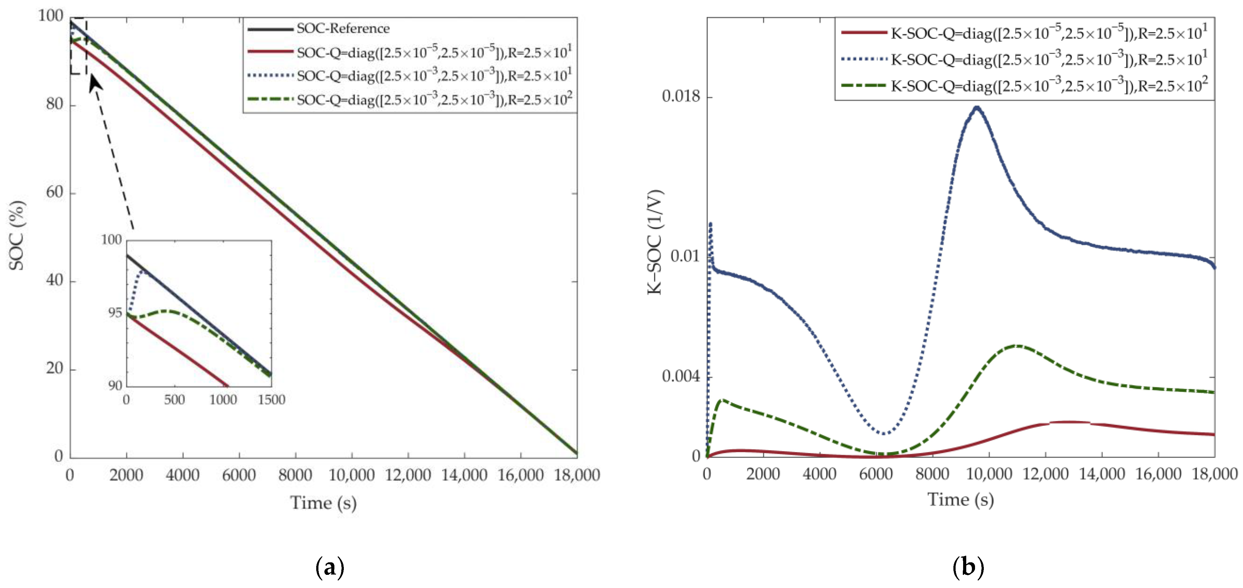
4.2.2. Q and R Matrices Design

The constant current condition is selected; the initial SOC is 0.99 and the initial SOC estimate is 0.95. The simulation results of discharge are as follows:

Figure 6 shows that, like the linear system, the adjustments of Q and R do have effects on the estimation. Reducing Q or increasing R within a certain range can improve the performance of the algorithm and the estimation accuracy. It can be seen from Figure 7 that the value of the Kalman gain becomes smaller and more stable when reducing Q or increasing R, which reduces the over-adjustment or under-adjustment of the algorithm and makes the estimation more accurate.

In addition, due to the initial error, it should be noted that the adjustment range of Q and R should be realistic. This is because the adjusted EKF is a suboptimal estimation algorithm which is equivalent to controlling the update intensity at each step.

It can be seen from Figure 8a that further increasing R to a certain value leads to a large deviation at the beginning of the SOC estimation curve, and the deviation increases with an increase in the initial error. This is because the Kalman gain K is too small at the beginning, as shown in Figure 8b. That is to say, the adjustment intensity at this period is less than the update intensity caused by the time update equation which is the ampere-hour integration of SOC. Therefore, the estimation curve appears to be almost parallel to the reference one. With the change of $c_k$, K increases, and the estimate gradually converges to the true value.

For Q, this phenomenon is not obvious, as shown in Figure 9. From the previous analysis, it can be explained by the observation that the influence of the process noise in the state equation is much smaller than that of the measurement noise. Therefore, the estimation performance is less sensitive to the adjustment of Q than the adjustment of R.

Q and R affect each other. As can be seen from Figure 10a, although most of the estimated curve from the beginning deviates from the reference one when Q = diag([2.5 × 10⁻⁵, 2.5 × 10⁻⁵]) and R = 2.5 × 10¹, increasing Q to diag([2.5 × 10⁻³, 2.5 × 10⁻³]) allows the estimation value to converge quickly. This is because the increase in R reduces the Kalman gain, but if Q increases simultaneously, this adverse effect can be eliminated, as shown in Figure 10b. As can be seen from Figure 10, even if R increases further to 2.5 × 10², Q = diag([2.5 × 10⁻³, 2.5 × 10⁻³]) is still big enough to provide adequate compensation.

5. Conclusions

This paper has explored the stability of the EKF-based observer for SOC estimation of the Lithium-ion battery. A fundamental analytical method of EKF for nonlinear systems was applied to analyze the error behavior of the observer. Numerical simulations were carried out to validate the influence of the system noises. The results showed that the voltage noise played a major role in the estimation. The dynamic influence of nonlinearity on the SOC estimation was illustrated by introducing the theory of steady-state KF algorithm. It is concluded that when the slope of the OCV-SOC curve is relatively large, the SOC estimation value is apt to converge, and when the slope of the OCV-SOC curve is small and changing, the SOC estimation error increases. The frequently used and high-efficiency range of SOC is located in the middle of the OCV-SOC curve, with a small and variable slope, and the voltage noise is inevitable. Therefore, it is sometimes challenging to accurately estimate the SOC of lithium-ion battery in the practical application. For the EKF-based SOC observer, the matrices Q and R can be used as design parameters, and the performance of the observer can be improved by adjusting Q and R.

SOC estimation has always been a hot topic in electric vehicle research. In recent years, published papers have made many beneficial attempts to explore new methods mainly based on complex nonlinear Kalman filter algorithms or neural networks. This paper wants to emphasize that, since the convergence of nonlinear system observer under noise conditions has not been theoretically guaranteed in general, it is necessary to analyze its stability in specific practical applications. In this way, the factors that affect the stability of the observer could be controlled in the design and use of the observer to achieve better performance. Otherwise, the error of nonlinear observer under noise conditions may sometimes become large or even diverge.

References

1. Szumanowski, A.; Chang, Y. Battery management system based on battery nonlinear dynamics modeling. IEEE Trans. Veh. Technol. 2008, 57, 1425–1432. [Google Scholar] [CrossRef]
2. Shi, D.; Zhao, J.; Wang, Z.; Zhao, H.; Eze, C.; Wang, J.; Lian, Y.; Burke, A.F. Cloud-Based Deep Learning for Co-Estimation of Battery State of Charge and State of Health. Energies 2023, 16, 3855. [Google Scholar] [CrossRef]
3. Plett, G.L. Extended Kalman filtering for battery management systems of LiPB-based HEV battery packs: Part 2. Modeling and identification. J. Power Sources 2004, 134, 262–276. [Google Scholar] [CrossRef]
4. Liu, X.T.; Li, K.; Wu, J.; He, Y.; Liu, X.T. An extended Kalman filter based data-driven method for state of charge estimation of Li-ion batteries. J. Energy Storage 2021, 40, 102655. [Google Scholar] [CrossRef]
5. Hossain, M.; Haque, M.E.; Arif, M.T. Online Model Parameter and State of Charge Estimation of Li-Ion Battery Using Unscented Kalman Filter Considering Effects of Temperatures and C-Rates. IEEE Trans. Energy Convers. 2022, 37, 2498–2511. [Google Scholar] [CrossRef]
6. Song, Y.; Grizzle, J.W. The Extended Kalman Filter as a local asymptotic observer for nonlinear discrete-time systems. In Proceedings of the American Control Conference, Chicago, IL, USA, 24–26 June 1992. [Google Scholar] [CrossRef]
7. Baras, J.S.; Bensoussan, A.; James, M.R. Dynamic Observers as Asymptotic Limits of Recursive Filters: Special Cases. SIAM J. Appl. Math. 1988, 48, 1147–1158. [Google Scholar] [CrossRef] [Green Version]
8. Lohmiller, W.; Slotine, J.J.E. On Contraction Analysis for Non-linear Systems. Automatica 1998, 34, 683–696. [Google Scholar] [CrossRef] [Green Version]
9. Lohmiller, W.; Slotine, J.J.E. Contraction analysis of non-linear distributed systems. Int. J. Control 2005, 78, 678–688. [Google Scholar] [CrossRef] [Green Version]
10. Boutayeb, M.; Rafaralahy, H.; Darouach, M. Convergence analysis of the Extended Kalman Filter used as an observer for nonlinear deterministic discrete-time systems. IEEE Trans. Autom. Control 1997, 42, 581–586. [Google Scholar] [CrossRef]
11. Reif, K.; Sonnemann, F.; Unbehauen, R. An EKF-Based nonlinear observer with a prescribed degree of stability. Automatics 1998, 34, 1119–1123. [Google Scholar] [CrossRef]
12. Reif, K.; Günther, S.; Yaz, E.; Unbehauen, R. Stochastic stability of the discrete-time Extended Kalman Filter. IEEE Trans. Autom. Control 1999, 44, 714–728. [Google Scholar] [CrossRef]
13. Reif, K.; Günther, S.; Yaz, E.; Unbehauen, R. Stochastic stability of the continuous-time Extended Kalman Filter. IEEE Proc.-Control Theory Appl. 2000, 147, 45–52. [Google Scholar] [CrossRef]
14. Waag, W.; Fleischer, C.; Sauer, D.U. On-line estimation of lithium-ion battery impedance parameters using a novel varied-parameters approach. J. Power Sources 2013, 237, 260–269. [Google Scholar] [CrossRef]
15. Baras, J.S.; Krishnaprasad, P.S. Dynamic observers as asymptotic limits of recursive filters. In Proceedings of the 21st IEEE Conference on Decision and Control, Orlando, FL, USA, 8–10 December 1982. [Google Scholar] [CrossRef]
16. Ljung, L. Asymptotic behavior of the extended Kalman filter as a parameter estimator for linear systems. IEEE Trans. Autom. Control 1979, 24, 36–50. [Google Scholar] [CrossRef] [Green Version]
17. Grizzle, J.W.; Moraal, P.E. Newton, observers and nonlinear discrete-time control. In Proceedings of the 29th IEEE Conference on Decision and Control, Honolulu, HI, USA, 5–7 December 1990. [Google Scholar] [CrossRef]
18. Boutayeb, M.; Aubry, D. A strong tracking extended Kalman observer for nonlinear discrete-time systems. IEEE Trans. Autom. Control 1999, 44, 1550–1556. [Google Scholar] [CrossRef]
19. Gauthier, J.; Bornard, G. Observability for any u(t) of a class of nonlinear systems. IEEE Trans. Autom. Control 1981, 26, 922–926. [Google Scholar] [CrossRef]
20. Dey, S.; Ayalew, B.; Pisu, P. Nonlinear Robust Observers for State-of-Charge Estimation of Lithium-Ion Cells Based on a Reduced Electrochemical Model. IEEE Trans. Control Syst. Technol. 2015, 23, 1935–1942. [Google Scholar] [CrossRef]
21. Lotfi, F.; Ziapour, S.; Faraji, F.; Taghirad, H.D. A switched SDRE filter for state of charge estimation of lithium-ion batteries. Electr. Power Energy Syst. 2019, 117, 105666. [Google Scholar] [CrossRef]
22. Casti, J.L. Recent Developments and Future Perspectives in Nonlinear System Theory. SIAM Rev. 1982, 24, 301–331. [Google Scholar] [CrossRef] [Green Version]
23. Lee, E.B.; Markus, L. Foundations of Optimal Control Theory; John Wiley and Sons, Inc.: New York, NY, USA, 1967. [Google Scholar]
24. Wang, X. Research on Observability of Nonlinear Systems Based on Linearization. Master’s Thesis, Harbin Institute of Technology, Harbin, China, 2009. [Google Scholar]
25. Yang, X.D.; He, P.; Hu, H.Z. The Performance Analysis of Kalman Filter. Tech. Autom. Appl. 1999, 18, 17–19. [Google Scholar] [CrossRef]
26. Deng, Z.L.; Yuan, G.; Mao, L.; Yun, L.; Hao, G. New approach to information fusion steady-state Kalman filtering. Automatica 2005, 41, 1695–1707. [Google Scholar] [CrossRef]
27. Chen, G.; Hsu, S.H. Linear Stochastic Control Systems; CRC Press: New York, NY, USA, 1995. [Google Scholar]
28. Rhudy, M.B.; Gu, Y. Online Stochastic Convergence Analysis of the Kalman Filter. Int. J. Stoch. Anal. 2013, 2013, 37–40. [Google Scholar] [CrossRef] [Green Version]
Figure 1. SOC curves under different voltage and current noise conditions: (a) different voltage noise conditions; (b) different current noise conditions.
Energies 16 05946 g001
Figure 2. SOC estimates using different sampling step sizes.
Energies 16 05946 g002
Figure 3. Curves of the element corresponding to SOC in the estimation error covariance matrix.
Energies 16 05946 g003
Figure 4. Simulation of discharge: (a) OCV curve; (b) SOC curve; (c) Curve of the element corresponding to SOC in the estimation error covariance matrix P k ; (d) Curve of the element corresponding to SOC in the coefficient matrix C k .
Energies 16 05946 g004
Figure 5. Simulation of ternary lithium-ion battery: (a) OCV curve; (b) SOC curve.
Energies 16 05946 g005
Figure 6. SOC results obtained by adjusting Q and R: (a) Adjusting Q; (b) Adjusting R.
Energies 16 05946 g006
Figure 7. Kalman gain obtained by adjusting Q and R: (a) Adjusting Q; (b) Adjusting R.
Energies 16 05946 g007
Figure 8. Simulation results with different initial estimates: (a) SOC; (b) Kalman gain.
Energies 16 05946 g008
Figure 9. Simulation results obtained by adjusting Q: (a) SOC; (b) Kalman gain.
Energies 16 05946 g009
Figure 10. Verification of the mutual influence between Q and R: (a) SOC; (b) Kalman gain.
Energies 16 05946 g010