Predicting Building Energy Demand and Retrofit Potentials Using New Climatic Stress Indices and Curves

Abstract

Building energy requalification in Italy and Europe has been much discussed in recent years due to the high percentage of existing buildings with poor energy performance. In this context, it is useful to obtain a user-friendly and fast tool to predict the thermal energy demand (TED) for space conditioning and the related primary energy consumption (PEC) as a function of climatic stress. In this study, the SLABE methodology (simulation-based large-scale uncertainty/sensitivity analysis of building energy performance) is used to simulate representative Italian buildings, varying parameters such as geometry, envelope and HVAC (heating, ventilating and space conditioning) systems. MATLAB^® in combination with EnergyPlus is used to analyze 200 buildings belonging to two structural types (multi-family buildings and apartment blocks) built in 1961–1975. Nine scenarios (as-built scenarios and eight retrofit ones) are investigated in 63 climatic locations. A regression analysis shows that the classical HDDs (heating degree days) approach cannot give an accurate prediction of TED because solar radiation is not accounted for. Thus, new climatic indices are developed alongside solar radiation, including the heating stress index (HSI), the cooling stress index (CSI) and the yearly climatic stress index (YCSI). The purpose of our work is to obtain climatic stress curves for the prediction of TED and PEC. Testing of this novel approach is performed by comparison with another building energy simulation tool, showing a low discrepancy, i.e., the coefficient of variation of the root mean square error is between 12% and 28%, which confirms certain reliability of the approach here proposed.

1. Introduction

Around the world, the building sector is responsible for around 37% of greenhouse emissions and 36% of final energy consumption, of which residential buildings account for about 61% [1]. These percentages are going to rise due to our growing world population [2]. In Europe alone, the final energy consumption share is nearly 43% [3], since most buildings were built before the introduction of mandatory laws about energy performance requirements [4]. For instance, in Italy, the first laws about the reduction of energy consumption in buildings date to the 1970s, but 25% of the residential stock was built before 1946 [5].

Moreover, considering the current war involving Russia and Ukraine, the issue of reducing fossil fuel consumption has become even more urgent. It is estimated that if all the European countries put into practice the defined guidelines for energy renovation [6] by 2040, buildings will be 40% more efficient than they are today [7], using less energy for heating and cooling. Minimizing the space conditioning demand of buildings is possible using appropriate models that can predict energy demands for heating and cooling since there is a correlation between the thermal energy demand for space conditioning (TED) or the related primary energy consumption (PEC) and the climatic condition in which the building is placed; this link can be denoted as climatic stress.

There are several parameters that describe the external climate, e.g., outdoor air temperature, relative humidity, solar radiation, wind speed, altitude and so on. Currently, the most used method for describing weather conditions is the degree-days method (DDs), due to its easy application [8]. This approach can provide the amplitude and frequency of the variable external temperature with respect to a reference temperature [9], usually defined as the outdoor temperature at which HVAC (heating, ventilating and air conditioning) systems should not work, ensuring comfortable indoor conditions. However, this technique can only give a partial description of climatic conditions that affect building performance since the impact of wind speed, solar radiation and humidity is not considered [10]. It is evident that these variables are fundamental in hot and humid areas, where latent loads and solar gains can highly affect building energy performance.

Several previous studies showed a linear relationship between TED and DD. For instance, De Rosa et al. [11] proposed a correction of cooling degree days (CDDs) that considers solar radiation, demonstrating that the linear relationship between TED and DD is maintained. Kohler et al. [12] defined a city-scale degree-day model, showing results’ discrepancies with different DD temperature definitions. According to Christenson et al. [13], the DD approach should be improved with new weather files that consider actual climate change. Thus, in order to obtain a more reliable prediction of heating and cooling demand, it is necessary to consider updated DD in addition to other parameters such as the yearly average outdoor temperature, the solar radiation or the latitude.

Some previous studies focused on climatic stress indices to predetermine the energy performance of buildings. In this vein, Park et al. [14] proposed an approach using the sol–air temperature in order to obtain the heat loads of an atrium space. Salmeron et al. [15] developed a comprehensive winter climatic severity index to predict heating demand, considering the number of sun hours besides HDDs; a comparison between the global energy performance of buildings in different climates was conducted to define a global climatic severity index, merging the winter and summer severity indices. Ciulla and D’amico [16] performed the assessment of energy demand for a designed high-energy performance building in fifteen different Italian cities using neural networks and multi-linear regression; the study showed simple correlations between thermal energy needs and the classical HDD. Neto et al. [17] used artificial neural networks based on EnergyPlus outputs to estimate the energy demand of the administration building of the University of Sao Paulo, considering solar radiation, external air temperature and air humidity. Andric and Al-Ghamdi [18] investigated the implication of climate change on residential buildings in Qatar, assuming, as a climatic stress index, the percentage of hours in which the outdoor air temperature is higher than 38 °C.

Furthermore, the proper definition of climatic stress indices, implying their classification in climatic zones according to the actual climatic conditions, is crucial to ensuring a proper differentiation of heating operation limits and energy efficiency regulations [19].

Paper Position

The present study aims to develop a new methodological approach to finding a correlation between the main building characteristics, thermal energy demand and climatic stress. Thus, the purpose is to obtain a user-friendly tool able to predict the building energy demand and to simplify and accelerate the initial planning for designers as a function of the climatic stress. This is one of the main novelties of this paper.

Various representative buildings of the Italian residential stock are simulated. The SLABE (simulation-based large-scale uncertainty/sensitivity analysis of building energy performance) methodology [20] is used to obtain a representative building sample (RBS). By varying the main characteristics, such as geometry and parameters of the building envelope, a set of 200 buildings is obtained. MATLAB^® and EnergyPlus are used together to simulate building energy performance for 63 Italian climatic locations that cover all of the national territory. With respect to the current literature, new climatic indices have been determined. They are HSI (heating stress index), CSI (cooling stress index) and YCSI (yearly climatic stress index), which all take into account solar radiation, which was not considered by most of the previous studies. Something similar was carried out by Ascione et al. [21] for the HSI, considering the latitude instead of the solar radiation but investigating only the thermal energy demand for heating. The present study puts together the heating and cooling demands to achieve the definition of a comprehensive stress index, YCSI. Then, the results are analyzed with a polynomial regression, relating HSI, CSI and YCSI to TED_h (TED for heating), TED_c (TED for cooling), and TED (TED_h + TED_c), respectively. Climatic stress curves are obtained considering different scenarios, with or without retrofit measures. Finally, a test of the proposed approach is carried out on an existing building.

2. Materials and Methods

This section mentions the well-known degree-days (DDs) method and then describes in detail the novel approach here proposed for predicting building energy demand and retrofit potentials using new climatic stress indices and curves. Finally, the case studies are delineated, i.e., representative building samples under different scenarios (as-built and retrofit solutions), as well as an existing residential building investigated to test the approach.

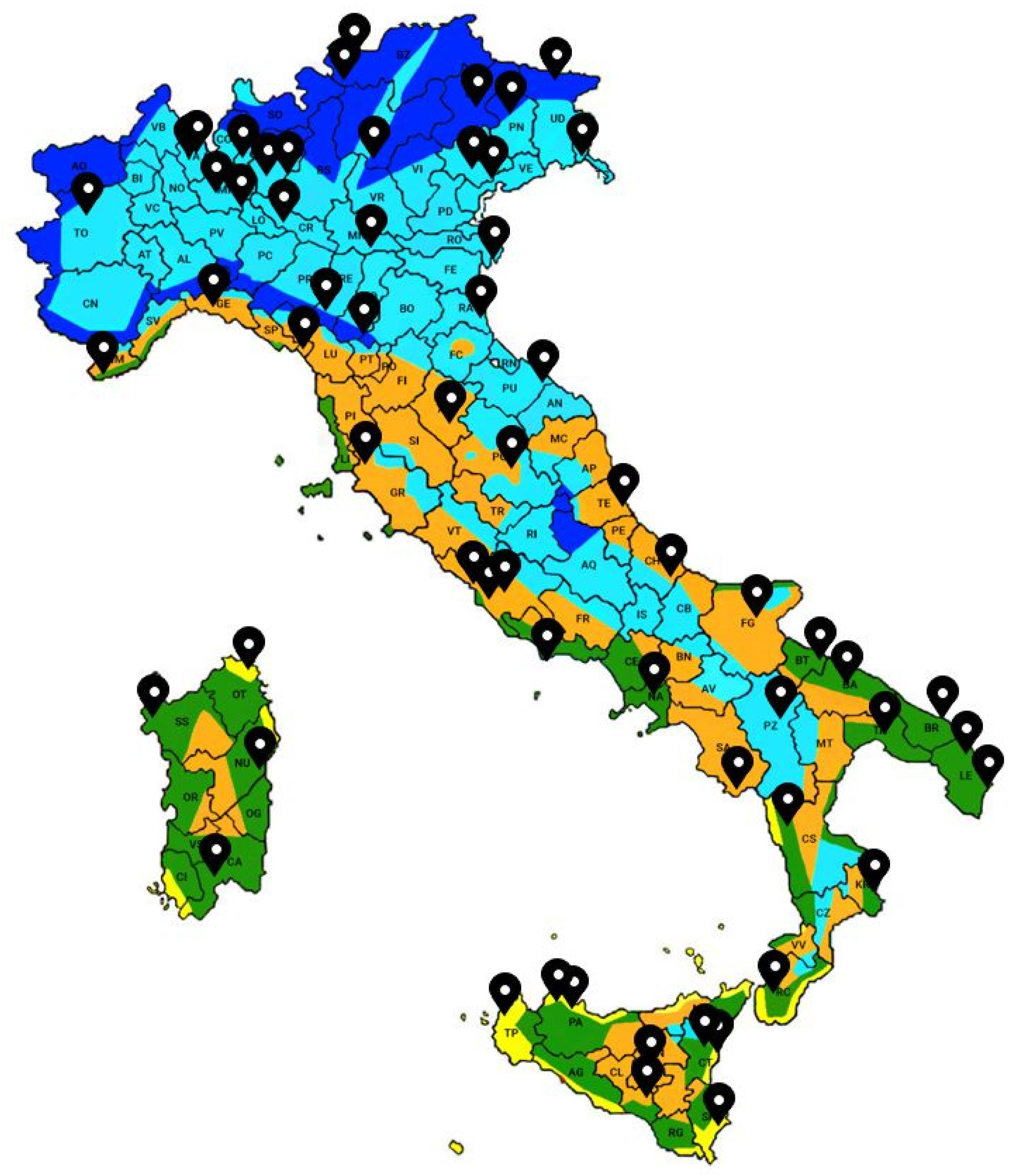
2.1. Degree-Days Approach: HDD and CDD

HDD is defined as shown in Equation (1). It depends on a base temperature T_b, in Italy set equal to 20 °C, and on the average external daily temperature T_e, where n is the number of days of the conventional heating period. In Italy, the latter starts with the first three days characterized by an average external temperature lower than 12 °C (indicated as T_winter) and ends with the first three days characterized by an average external temperature higher than 12 °C. Only positive differences are taken into account. T_b represents the comfort temperature, i.e., the one that ensures occupants’ thermal comfort when the HVAC (heating, ventilating and space conditioning) system is switched off.

$$HDD={\displaystyle \sum }_{e=1}^{n\to heating season }{\left(T_b-T_e\right)}^{+}$$

(1)

In Italy, the HDD is binding for the HVAC system design and for the definition of the heating period, as well as for the definition of several limit values for minimum energy requirements [22]. According to the Italian law [23], six climatic zones, from A to F, from the warmest to the coldest, are defined based on HDDs, implying different heating operation limits, as reported below (not considering the temporary changes implemented in 2022 as for the heating operation limits):

• zone A, from 0 to 600 heating degree days (HDDs); the heating season is from 1 December to 15 March, and the heating system can be switched on for 6 h per day;
• zone B, from 601 to 900 HDDs; the heating season is from 1 December to 31 March and the system can be switched on for 8 h per day;
• zone C, from 901 to 1400 HDDs; the heating season is from 15 November to 31 March, and the system can be switched on for 10 h per day;
• zone D, from 1401 to 2100 HDDs; the heating season is from 1 November to 15 April, and the system can be switched on for 12 h per day;
• zone E, from 2101 to 3000 HDDs; the heating season is from 15 October to 15 April, and the system can be switched on for 14 h per day;
• zone F, HDDs higher than 3000; there are no limits to heating operation.

In regard to CDD, the approach is similar (see Equation (2)), but the temperature differences are assessed when the external temperature exceeds the T_b during the cooling period. Since space cooling is linked to solar radiation, which is an extremely variable parameter, the dynamic behavior of the HVAC-building system is not determined in an accurate way; the CDD approach is not as reliable as the HDD one.

$$CDD={\displaystyle \sum }_{e=1}^{n\to cooling season}{\left(T_e-T_b\right)}^{+}$$

(2)

Although there are more updated national climate data standards [24], presently the legally recognized HDDs in Italy refer to climate data dating back to 1994, and CDD values are not defined.

2.2. Proposed Novel Approach: HSI, CSI and YCSI

In this study, optimization for defining new climate stress indices, more evolved than DD, is carried out. They include solar radiation and can consider current climate changes too, an issue not covered by the actual normative values. They are HSI (heating stress index), CSI (cooling stress index) and YCSI (yearly climatic stress index). The optimization consists of finding the expressions of these indices that provide the best polynomial regression with thermal energy demands.

The HSI is calculated in the same way as HDD, but using the sol–air temperature (T_sol-air) instead of the external one and diversified according to the individual city/municipality, as illustrated in [25]. Since the current Italian normative values do not take solar radiation into account, the HDD is calculated with reference only to the external temperature. In the proposed approach, the HSI is determined using the sol–air temperature; solar radiation is a fundamental parameter since it can significantly affect the heating and cooling needs of the building-plant system with lag and attenuation phenomena. The sol–air temperature is the external air temperature that would bring the same heat flux to the external surface of a wall as in reality due to the combined effect of incident solar radiation and adduction with the external air. Thus, the solar irradiance G is taken into account. The sol–air temperature is defined as in Equation (3).

$$T_{sol–air}=T_e+G\ast \frac{{\alpha }_{sol}}{h_e}$$

(3)

where α_sol is the solar radiation absorption coefficient and indicates the ability of the material to absorb the incident radiant solar energy; generally, dark and rough surfaces get hotter than light and smooth ones; and h_e is the external adduction conductance, which characterizes the heat transfer between the surface and the external air. For the calculation, α_sol is assumed to be equal to 0.5 and h_e to 25 W/m²K, as recommended by Italian standards [26].

The sol–air temperature was introduced in [27] and was used by Erbs et al. [28] to calculate sol–air heating and cooling degree days.

In this way, solar radiation is taken into account, overcoming the great limit of HDDs and maintaining the dependence on T_b and T_winter.

As concerns CSI, the approach is similar, but with reference to the cooling season. In this case, T_summer is the outdoor air temperature that corresponds to the start of the cooling season.

YCSI is a function of HSI and CSI. With the aid of MATLAB^®, two possible best expressions are defined (Equations (4) and (5)). They consider the possibility that HSI and CSI have different orders of magnitude, which would not allow a classic sum between them, which would in fact be poorly representative of the real case.

$$YCSI=\frac{HSI*CSI}{{\left(HSI*CSI\right)}_{MAX}}$$

(4)

$$YCSI=a_1*\frac{HSI}{HS{I}_{MAX}}+a_2*\frac{CSI}{CS{I}_{MAX}}$$

(5)

where a₁ and a₂ are the coefficients of the considered expression and provide further decision variables for the optimization problem.

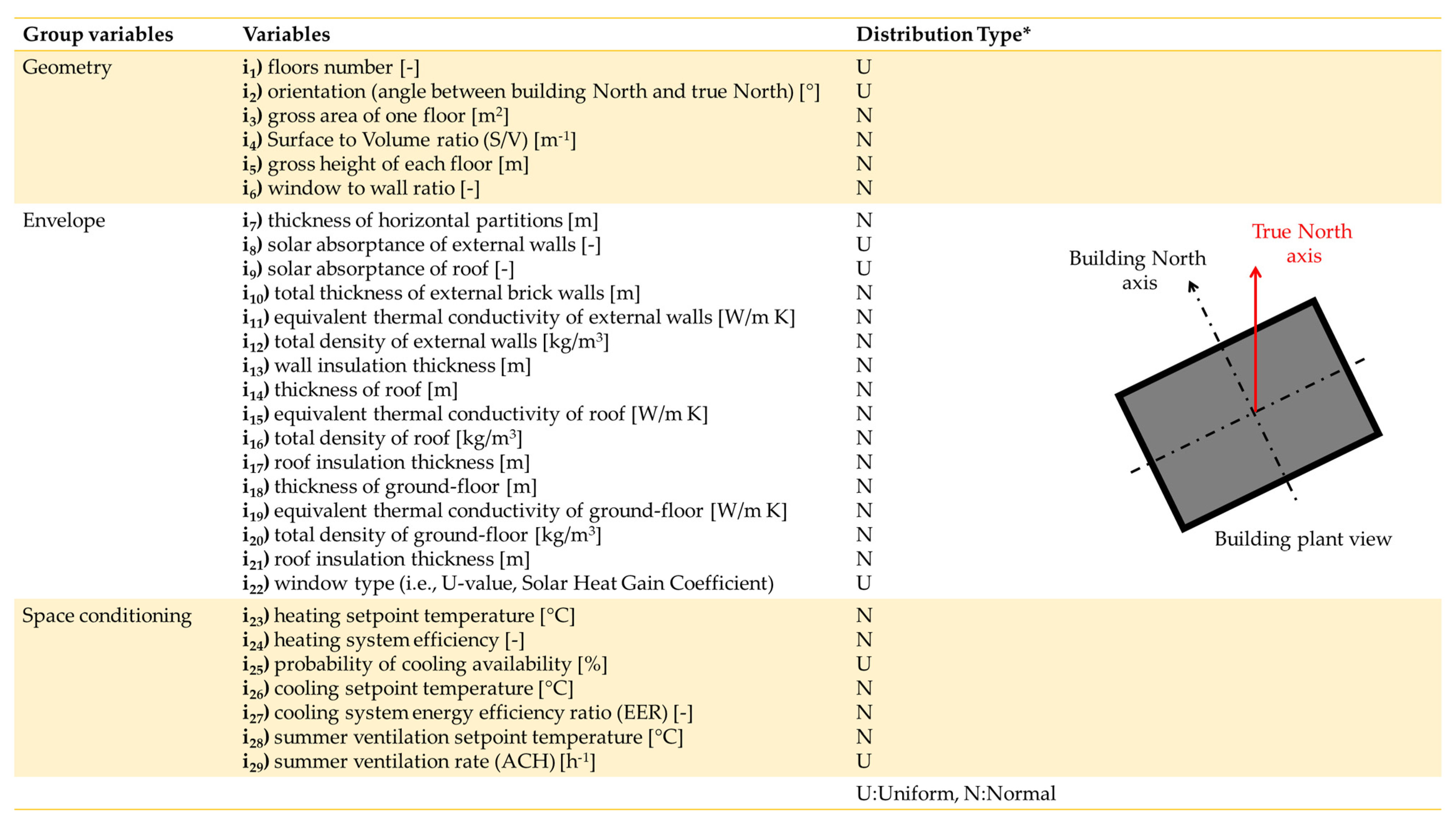
2.3. SLABE and Optimization of HSI, CSI and YCSI

The SLABE (simulation-based large-scale uncertainty/sensitivity analysis of building energy performance) methodology [20] enables the creation of a representative building sample (RBS) starting from only two buildings: a reference multi-family building (RBS-a) and a reference apartment block (RBS-b). The union of the two building samples deriving from the base buildings considered is made up of 200 buildings. More specifically, the RBS-a is obtained from the multi-family building by varying its geometry, stratigraphy and characteristics of the HVAC (heating, ventilating and air conditioning) system; the RBS-a is made up of 100 buildings. The same approach is used for the RBS-b, which refers to apartment blocks.

Notably, a bottom-up modeling approach is implemented—within a Monte Carlo framework via Latin hypercube sampling (LHS)—which enables accurate energy simulations while comprehending the uncertainties too. The energy performance of the RBS is simulated via EMAR [29], in which MATLAB^® and EnergyPlus work together: MATLAB^® creates an Energy Plus model from numerical inputs and runs the simulation in the EnergyPlus environment, then imports and post-processes the simulation outputs to assess performance indicators related to building energy needs.

As already mentioned, using the degree days is not a comprehensive solution to characterizing climate stress. Thus, as mentioned, this study proposes new indicators, i.e., HSI, CSI and YCSI, that consider solar radiation through the sol–air temperature. The expressions of such indicators are optimized to achieve the best correlations, performing polynomial regressions with:

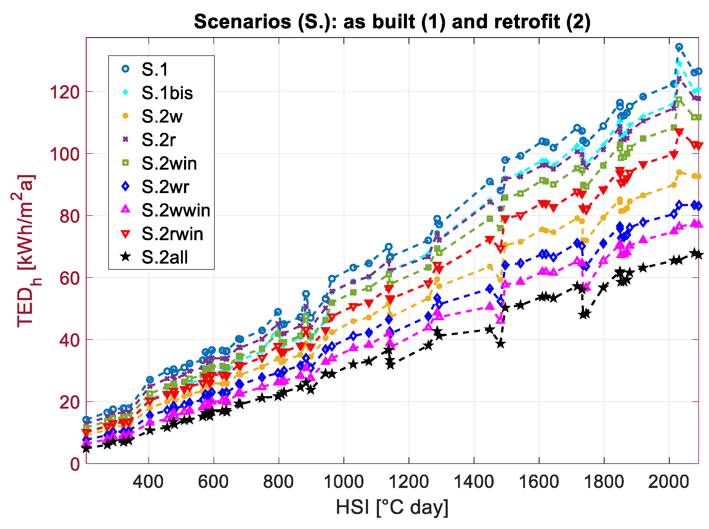
• thermal energy demand for space heating (TED_h) as concerns HSI;
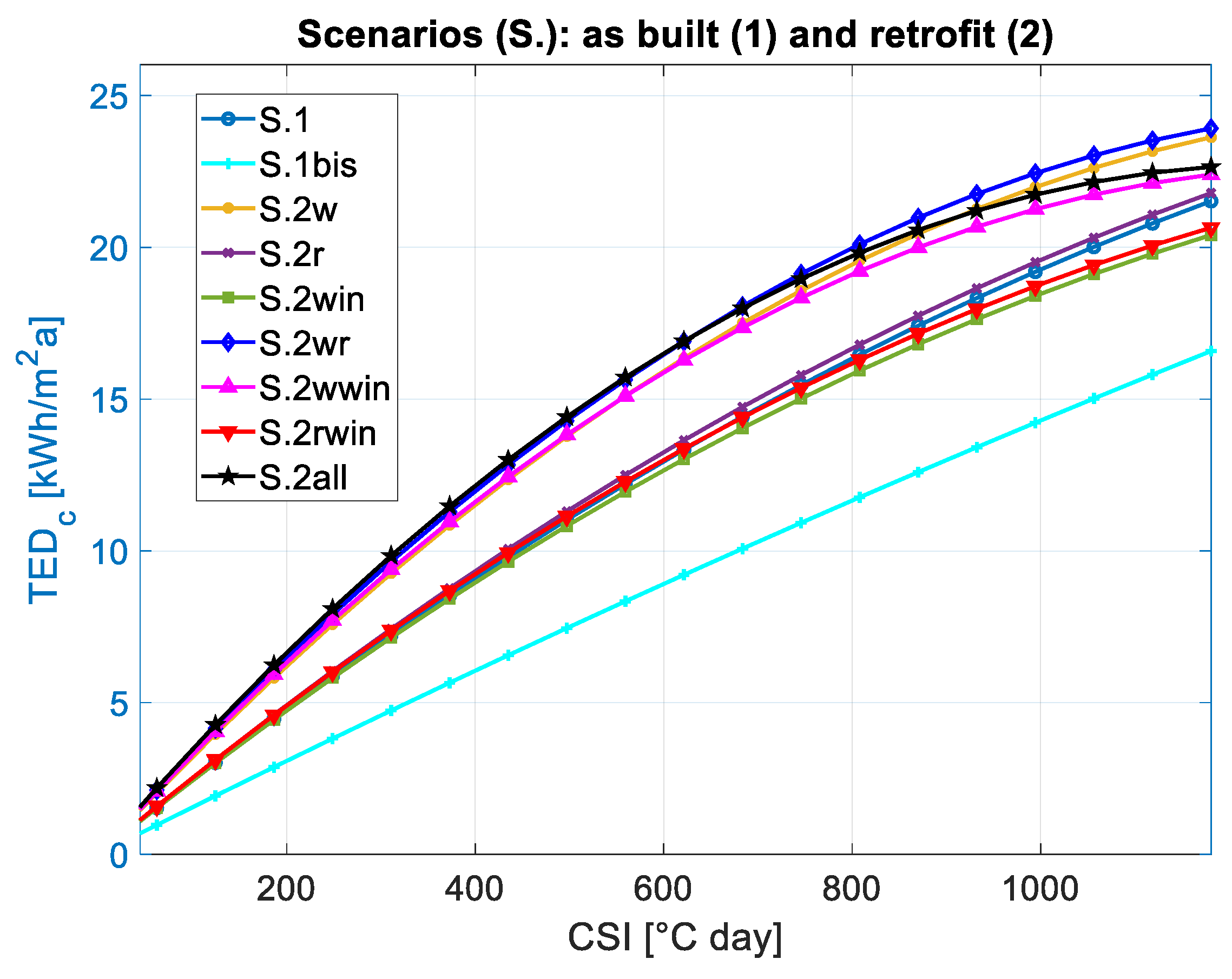
• thermal energy demand for space cooling (TED_c) as concerns CSI;
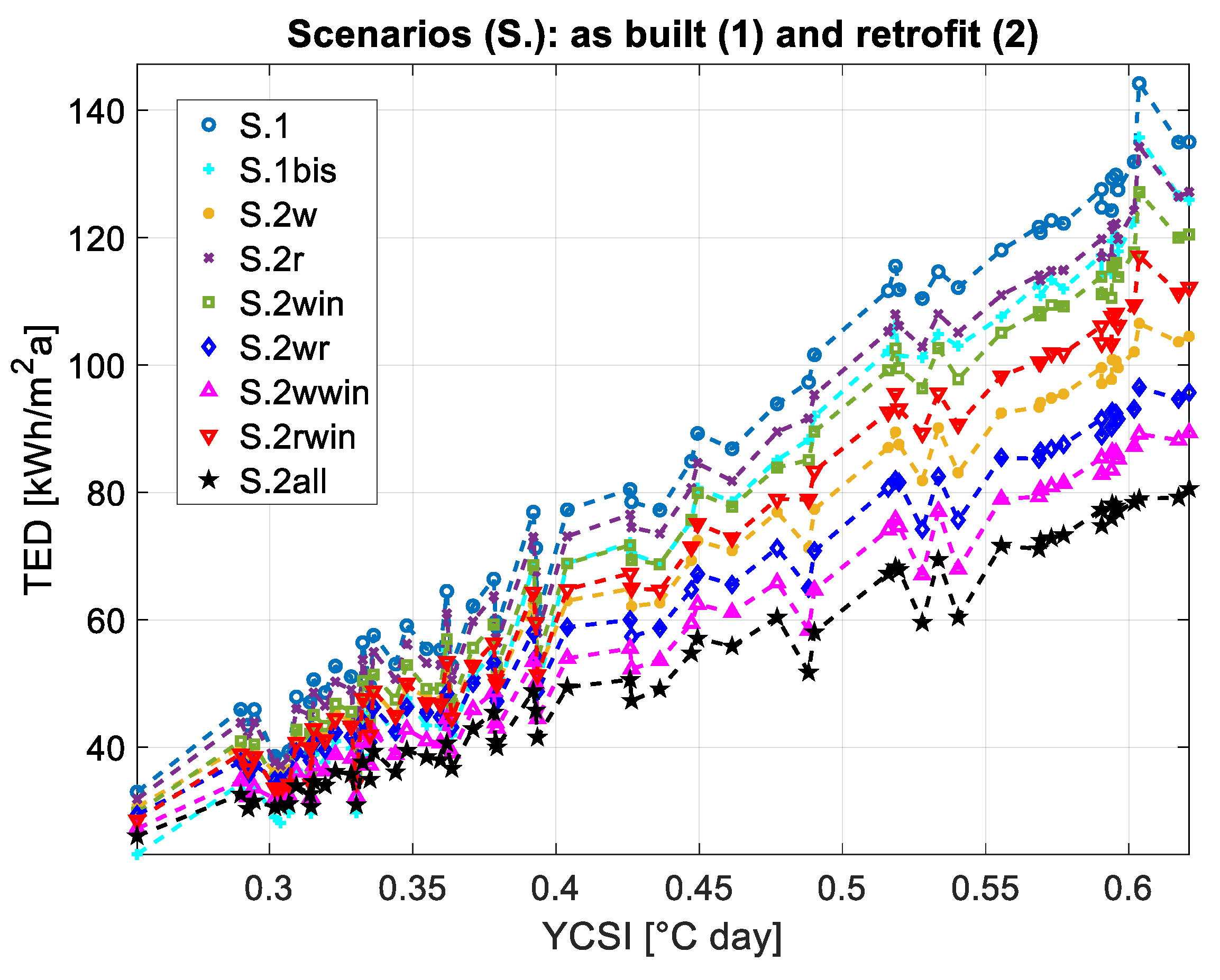
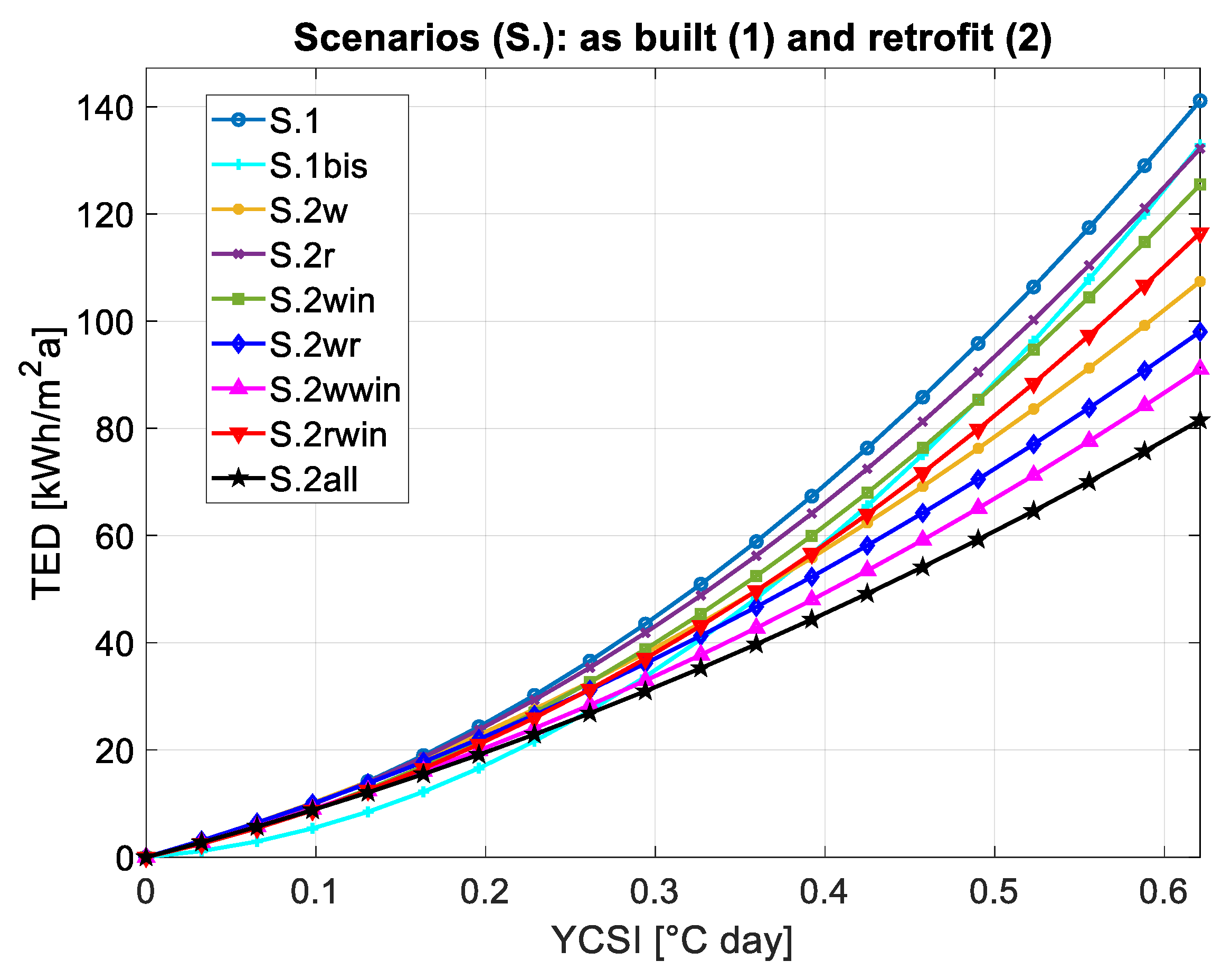
• total thermal energy demand for space conditioning (TED = TED_c + TED_h) as concerns YCSI.

The optimization problem is solved via an exhaustive search, i.e., brute-force optimization, where all possible combinations of the vector, including the decision (or design) variables, are analyzed. The decision variables are integer numbers, whose variability is defined as follows:

• for HSI, the decision variables are T_b, T_winter and the polynomial order (1st or 2nd) of the regression with TED_h: both temperature values vary in the range 10–20 °C, with a step of 1 °C;
• for CSI, the decision variables are T_b, T_summer and the polynomial order (1st or 2nd) of the regression with TED_c: both temperature values vary in the range 15–24 °C, with a step of 1 °C;
• for YCSI, the expression type, i.e., Equation (4) or Equation (5), and for the latter the coefficients a₁ and a₂, which vary between 0 and 1 with a step of 0.05; in both equations, the achieved optimal expressions of HSI and CSI are used.

The temperature variations of the decision variables T_b and T_winter are set considering the values defined by the national legislation [23] and investigating their surroundings. Thanks to this approach, the analytical expression of a new comprehensive index, YCSI, never proposed in the literature, is defined in this study.

The considered objective functions are the regression indicators, i.e., the determination coefficient R² to be maximized and the coefficient of variation of the root mean square error cv(RMSE) to be minimized. The equations of these regression indices are reported in Equations (6) and (7).

$$R^2=1-\frac{{{\displaystyle \sum }}_{i=1}^N{\left(x_i-y_i\right)}^2}{{{\displaystyle \sum }}_{i=1}^N{\left(x_i-\overline{x}\right)}^2}$$

(6)

$$cv\left(RMSE\right)=\frac{1}{\overline{x}}·\sqrt{\frac{1}{N}{\displaystyle \sum }_{i=1}^N{\left(x_i-y_i\right)}^2}$$

(7)

Notably, a mono-objective optimization approach is conducted in order to maximize the objective function R², which is equivalent to minimizing the cv(RMSE) value.

The values of R² and of cv(RMSE) derive from EnergyPlus outputs related to building thermal energy demand; it is possible to read these indices among the results of the polynomial regression performed to obtain the climatic stress curves.

2.3.1. As-Built Scenario (S.1)

The scenario considers 200 buildings, 63 climatic locations and 29 parameters. The considered locations cover the whole Italian territory and typical climate conditions, as shown in Figure 1.

The 29 parameters are divided into three groups related to geometry (i₁–i₆), envelope (i₇–i₂₂) and space conditioning (i₂₃–i₂₉), as shown in Figure 1. Each building has its own characteristics (e.g., S/V ratio, U-value of external walls, ground floor, roof, and windows) deducted from the TABULA project [30,31]. The U-value indicates the thermal transmittance of envelope components. The TABULA project has been used as a reference for defining building HVAC typologies in other studies [32]. It synthesizes the Italian residential building stock with the most recurring structures in various periods; the one considered in this study is from 1961 to 1975. Notably, the two building samples RBS-a and RBS-b are generated via large-scale uncertainty analysis (SLABE) from the reference buildings of TABULA for multi-family buildings and apartment blocks, respectively, built in Italy in such a period. The structure of both buildings is reinforced concrete and hollow bricks without thermal insulation, implying high U-values, as shown in

Table 1. Reference buildings of TABULA [30,31], built in Italy in the period 1961–1975.

Building	S/V [m−1]	U Walls [W/m2K]	U Ground-Floor [W/m2K]	U Roof [W/m2K]	U Windows [W/m2K]	Solar Heat Gain Coefficient [-]
Multi-family building	0.54	1.15	1.30	1.42	4.90	0.85
Apartment block	0.46	1.10	1.30	1.42	4.90	0.85

. All buildings are characterized by a centralized traditional natural gas-fired boiler for space heating, while only 50% of the apartments are equipped with electric split-type air conditioners for space cooling. For each location, the heating operation schedules comply with the heating period and maximum hours per day, as defined by Italian regulations [23]. On the other hand, the schedule for cooling operations is the same for all locations, considering that cooling systems can always be switched on during the summer season since national regulations do not limit their use. There are no renewable energy sources. The building use, occupation, operation of electric equipment, and artificial lighting are set according to the typical values and schedules of residential buildings. Given that two typologies of windows have been implemented (i₂₂ in

Table 2. Variation ranges of the input variables for the generation of the RBS (k is the equivalent thermal conductivity, ρ is the component density, SHGC is the solar heat gain coefficient, and PVC is polyvinyl chloride).

Variable (i)	Value for RBS-a	Value for RBS-b
(i1) floors number	4, 5, 6	7, 8, 9
(i2) orientation	angle between building N and true N: 0°, +45°, −45°, 90°
(i3) gross area per floor	from 150 to 350 m2	From 300 to 500 m2
(i4) S/V	from 0.80*TABULA-value to 1.20*TABULA value [m−1]
(i5) gross height per floor	from 2.80 to 3.80 m
(i6) window-to-wall ratio	from 0.10 to 0.30
(i7) wall thickness	from 0.20 to 0.35 m
(i8) wall solar absorbance	from 0.10 to 0.90
(i9) roof solar absorbance	from 0.10 to 0.90
(i10) wall brick thickness	from 0.18 to 0.25 m	From 0.18 to 0.30 m
(i11) k of walls	0.30, 0.36, 0.43, 0.50 W/m K
(i12) ρ of external walls	600 kg/m3 for k = 0.30 W/m K, 800 kg/m3 for k = 0.30 W/m K, 1000 kg/m3 for k = 0.43 W/m K, 1200 kg/m3 for k = 0.50 W/m K
(i13) wall insulation thickness	-
(i14) roof thickness	from 0.25 to 0.40 m
(i15) k of roof	0.43, 0.50, 0.59, 0.72 W/m K
(i16) ρ of roof	1000 kg/m3 for k = 0.43 W/m K, 1200 kg/m3 for k = 0.50 W/m K, 1400 kg/m3 for k = 0.59 W/m K, 1600 kg/m3 for k = 0.72 W/m K
(i17) roof insulation thickness	-
(i18) ground-floor thickness	from 0.25 to 0.40 m
(i19) k of ground-floor	(see i15)
(i20) ρ of ground-floor	(see i16)
(i21) ground-floor insulation thickness	-
(i22) window type	single-glazed with a wooden frame with U = 4.90 W/m2K and SHGC = 0.85 or double-glazed air-filled with a PVC frame with U = 2.80 W/m2K and SHGC = 0.76 (considering a window replacement probability of 50% for some apartments)
(i23) heating set-point temperature (T)	19, 19.5, 20, 20.5, 21 °C
(i24) heating efficiency	from 0.60 to 0.90
(i25) cooling probability	50%
(i26) cooling set-point T	25, 25.5, 26, 26.5, 27 °C
(i27) cooling energy efficiency ratio	from 2.00 to 3.00
(i28) summer ventilation set-point T	26, 26.5, 27, 27.5, 28 °C
(i29) summer ventilation ACH	from 2 to 6 h−1

), the infiltration rate is set equal to 0.75 h⁻¹ when single-glazed windows are present, whereas it is 0.50 h⁻¹ when double-glazed windows are installed because of the higher air-tightness.

The two RBSs are generated from the TABULA reference buildings, varying the input variables reported in Figure 2 using uniform or normal distributions as in [20] and the variation ranges delineated in Table 2. A uniform distribution is used when the variable has the same probability of having any value in the range, whereas a normal distribution is used when the probability of having the average value in the range is higher. Some examples are reported just below. The total thickness of the vertical walls’ bricks (variable i₁₀) ranges between 0.18 and 0.25 m for RBS-a and between 0.18 and 0.30 m for RBS-b. Such ranges have been determined to achieve a mean value of the walls’ U-value around the TABULA value, i.e., 1.15 W/m²K in the former case and 1.10 W/m²K in the latter. The variable i₁₁, that is, the equivalent thermal conductivity of external walls’ bricks, can assume the values 0.30, 0.36, 0.43 and 0.50 W/m K, according to typical hollow bricks. The same is true for the variable i₁₂, the total density of external walls: typical values associated with the mentioned thermal conductivity values are considered. The same occurs for the variable i₁₆. The efficiency (variable i₂₄) of the heating system (centralized traditional natural gas and radiators) related to the lower heating value ranges between 0.60 and 0.90 to take into account the presence of both old and new boilers (installed in the last few years). The mean value of the considered range is around the value provided by TABULA. Similarly, the nominal energy efficiency ratio (EER) of the cooling system (electric air-cooled chiller) ranges between 2 and 3 (variable i₂₇) to take into account the presence of both old and new chillers.

2.3.2. Retrofit Scenarios (S.2)

This study investigates energy retrofit scenarios in addition to S.1:

• S.1bis: it is similar to S.1, but with the heating set-point temperature (i₂₃) reduced by 1 °C and the cooling set-point temperature (i₂₆) increased by 1 °C for energy efficiency reasons;
• S.2w: it considers the insulation of external walls, thus modifying the variable i₁₃ to achieve the U-value defined by the law in force [22] depending on the climatic zone;
• S.2r: it considers the insulation of the roof, thus modifying the variable i₁₇ to achieve the U-value defined by the law in force [22] depending on the climatic zone;
• S.2win: it considers the replacement of the windows (in terms of both frame and glass), thus modifying the variable i₂₂, with double-glazed argon-filled low-emissive windows with PVC frames, U = 1.40 W/m²K and SHGC = 0.56, complying with the Italian law in force [22] for all climatic zones;
• S.2wr: it considers the insulation of both external walls and the roof;
• S.2wwin: it considers the replacement of the windows and the insulation of external walls;
• S.2rwin: it considers the replacement of the windows and the insulation of the roof;
• S.2all: it considers the replacement of the windows and the insulation of both the external walls and the roof, thus modifying the variables i₂₂, i₁₃ and i₁₇.

The considered thermal insulation material is polyurethane, with a thermal conductivity of 0.026 W/m K. The retrofit scenarios have been defined based on the authors’ expertise, considering the most widespread measures on the market usually applied in the national territory, in order to fulfil the minimum energy performance requirements defined by current legislation [22]. It is noticed that such common retrofit measures mainly address the reduction of heating demand, which is popular in balanced climates. Several scientific studies show that the choice of solutions for the energy design/retrofit of buildings often involves competing criteria [33,34], which are outside the scope of this study.

The scenarios investigated are a total of nine, considering the as-built scenario too. In all scenarios, the weather data files for the 63 Italian locations considered come from the collection IGDG “Gianni De Giorgio”, available on the website of EnergyPlus [35]. They cover all typical Italian climates.

2.4. Testing Case Study: An Existing Building

TerMUS Plus^® v.1 (ACCA software) is a tool by for the dynamic energy simulation of buildings that integrates the high capability of the EnergyPlus calculation engine with the simplicity of BIM-3D modeling in a single solution. It is used for investigating an existing residential building as a case study to test the proposed approach. The building has four floors above ground. The net height per floor is equal to 3.20 m, and the net floor area is 163.4 m². Its main thermal characteristics are synthesized below:

• Perimetral walls in tuff blocks: U = 0.66 W/m²K at the ground floor, U = 0.87 W/m²K at the first and second floors, and U = 1.13 W/m²K at the top floor;
• Inter-floor slab in masonry: U = 1.20 W/m²K;
• Ground floor as crawl space: U = 1.61 W/m²K;
• Attic floor in masonry: U = 0.98 W/m²K;
• Sloping roof with terracotta tiles: U = 1.88 W/m²K;
• Double-glazed windows air-filled with pine wood frames: U = 2.81 W/m²K.

As regards the HVAC system, on each floor there is a natural gas boiler (with an average efficiency of 80%) that supplies energy for heating and domestic hot water. The emission subsystem is made up of aluminum radiators. In the building, there is neither controlled ventilation nor a cooling system.

The building is simulated in different locations, belonging to the Italian climatic zones B, C, D and E, excluding zones A and F, which are less representative. As shown in

Table 3. Considered climatic locations for the testing case study.

Climatic Zones	HDD [°C Day] Ranges for Each Climatic Zone			Considered Locations	HDD * [°C Day]
B		from 600	to 900
	1/3 of the range	700		Palermo-Punta Cinisi	643
	2/3 of the range	800		Trapani-Birgi	799
C		from 901	to 1400
	1/3 of the range	1067		Lecce-Galatina	1050
	2/3 of the range	1233		Roma-Fiumicino	1342
D		from 1401	to 2100
	1/3 of the range	1633		Grosseto	1660
	2/3 of the range	1867		Ancona-Falconara	1913
E		from 2101	to 3000
	1/3 of the range	2400		Bologna-Borgo Pan.	2423
	2/3 of the range	2700		Piacenza	2719

* The HDD values are assessed from the IGDG weather data files and do not correspond to the normative values.

, for each zone, two locations are chosen, with HDD values close to 1/3 and 2/3 of the related zone HDD ranges, respectively. The period in which the heating system is switched on as well as the maximum hour per day are set as defined by the national legislation [23] with reference to the climatic zone analyzed. In the building, an occupancy density of 0.03 people/m² is set, assuming a metabolic rate of 126 W/person. The occupation schedule is characterized by standard residential weekdays, during which the minimum occupation rate is 20% (working hours), and weekends, where the minimum occupation rate is 80%. The natural ventilation rate is set at 0.5 h⁻¹.

The retrofit measures are the same as described in Section 2.3.

3. Results and Discussion

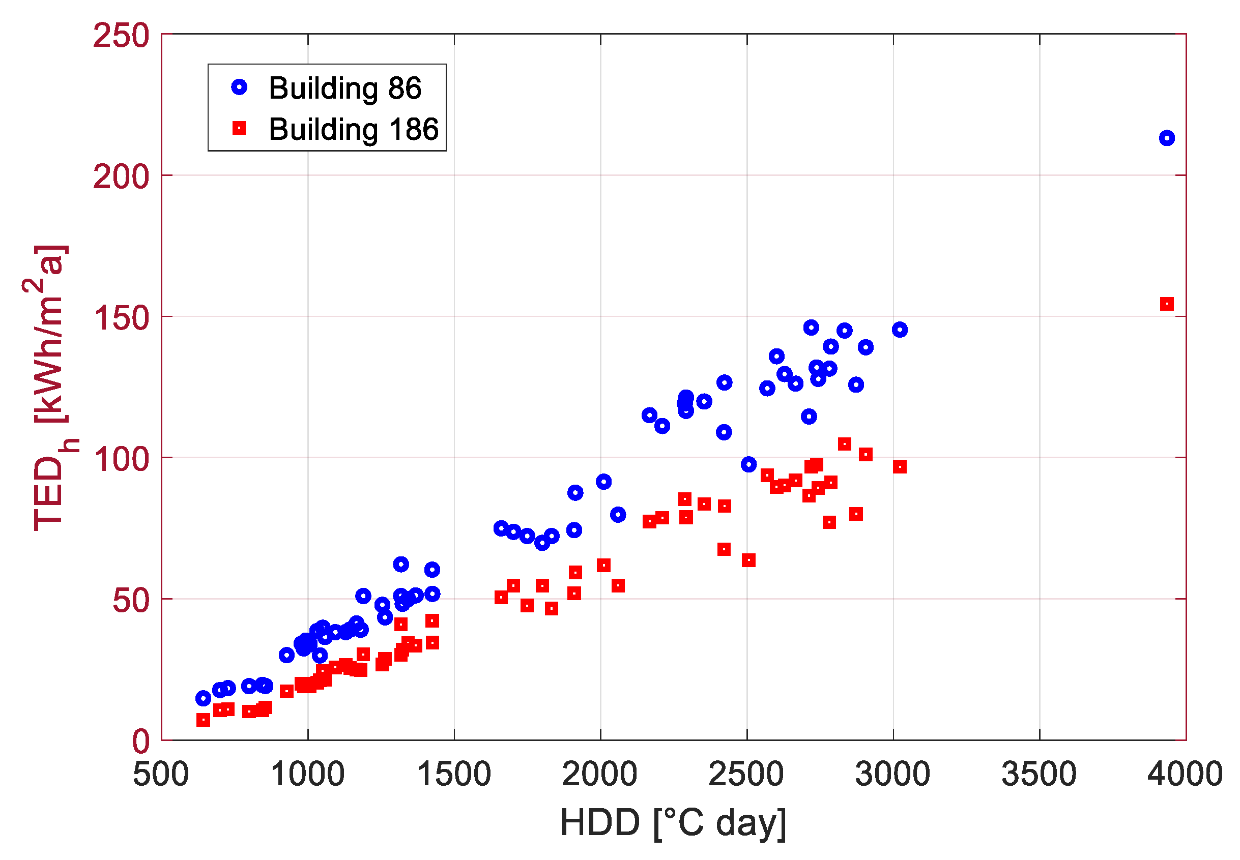
3.1. Limits of the Classical HDD Approach

Figure 3 depicts TED_h (thermal energy demand for heating) as a function of HDDs (heating degree days) of all 63 Italian locations investigated for two buildings of the simulated RBS (representative building sample). Note that the HDD values are assessed from the IGDG weather data files and do not correspond to the normative values, which refer to climatic data different from those used in the simulations. The two buildings are randomly chosen for the RBS: building n.86 belongs to the RBS-a (multi-family buildings), while building n.186 belongs to the RBS-b (apartment blocks). It should be noted that the discrepancy between the two point clouds becomes more marked going from warmer (lower HDDs) to colder (higher HDDs) climates. The building n.186 shows lower TED_h values than the other building since it has a lower S/V ratio; in other words, it disperses less thermal energy through its envelope at the same gross volume.

For each building, there are significant differences in TED_h at the same HDD value, i.e., by considering a vertical line. The same occurs for the other buildings of the RBS. This shows that HDD is not an exhaustive and effective climatic index to predict the thermal energy demand of a building because it does not include the solar radiation contribution, which can lead to significant differences in building energy needs for locations characterized by similar trends in the external temperature [21].

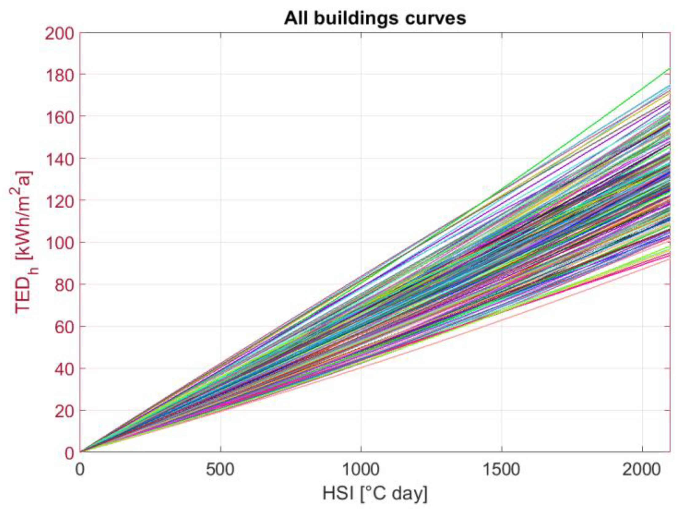
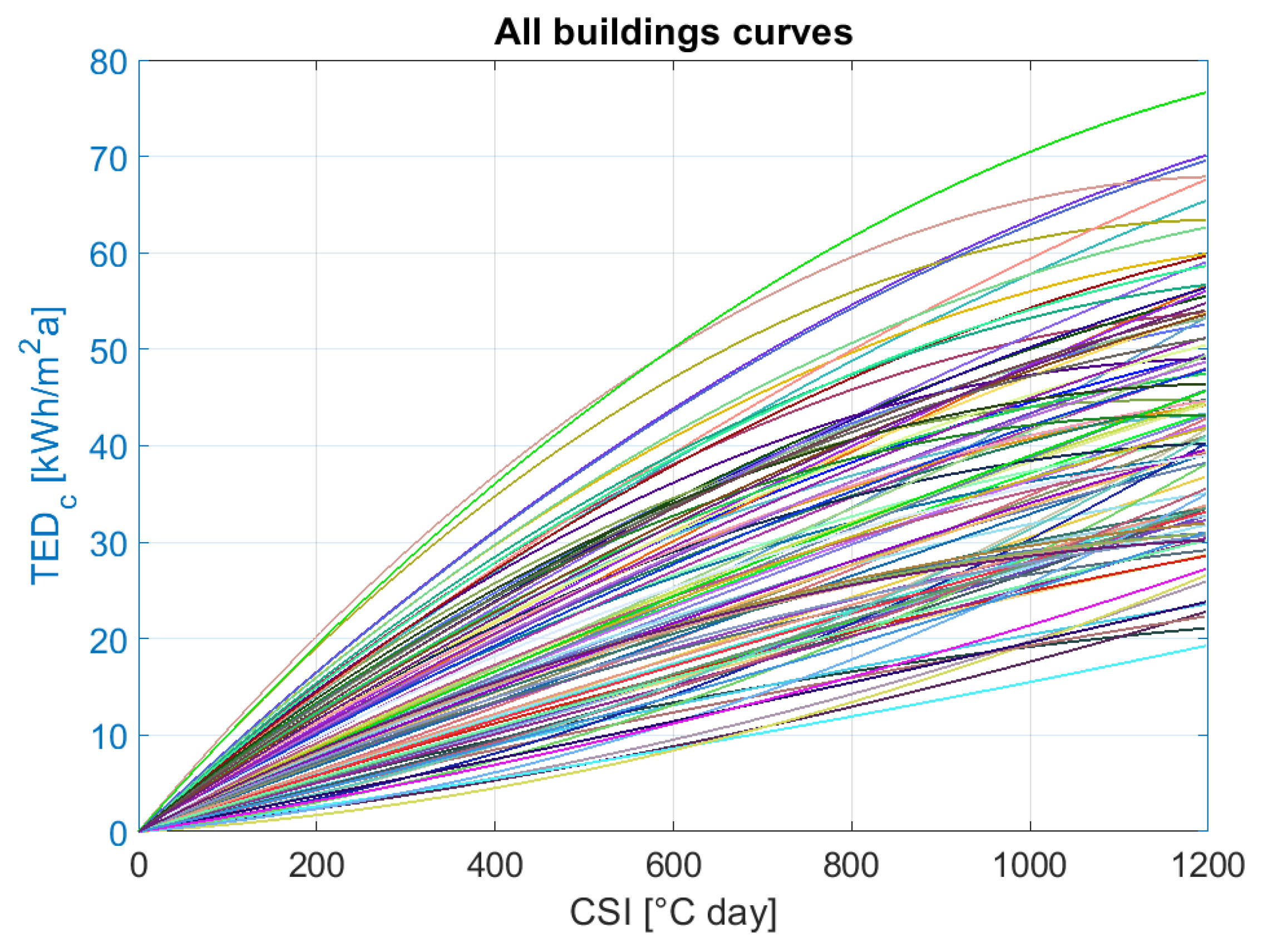
3.2. HSI, CSI and YCSI Polynomial Regressions

This subsection focuses on the novel climatic stress indices proposed, i.e., HSI (heating stress index), CSI (cooling stress index) and YCSI (yearly climatic stress index), achieved through the brute-force (exhaustive search) optimization process described in Section 2.3. Notably, the figures below represent the following polynomial regressions of the 2nd order for all the buildings of the RBS:

• Figure 4: TED_h (thermal energy demand for heating) vs. HSI;
• Figure 5: TED_c (thermal energy demand for cooling) vs. CSI;
• Figure 6: TED (TED_h + TED_c) vs. YCSI.

The main parameters that make the difference among the curves are above the floor number (i₁) and the gross area of each floor (i₃) belonging to the geometry group variables, and the heating and cooling set-point temperatures (i₂₄ and i_26, respectively) belonging to the space conditioning variable group.

The expressions of the climatic indices minimize the cv(RMSE) (coefficient of variation of the root mean square error) and maximize the R² (coefficient of determination) between the polynomial regressions and SLABE (i.e., EnergyPlus) outputs. The methodology used is based on the sol–air temperature, which is higher than the external air temperature. Making a comparison between the classical degree-days method and the new approach, better results are obtained in favor of the new indices, with a higher R² and a lower cv(RMSE).

The results for the optimal HSI expression are as follows:

• A 2nd order polynomial regression;
• Base temperature for degree-day assessment: T_b = 17 °C;
• Temperature for the start of the heating season: T_winter = 17 °C.

The regression indicators are as follows: R² equals 0.989, RMSE equals 3.44 kWh/m²a and cv(RMSE) equals 5.18%.

The results for the optimal CSI expression are as follows:

• A 2nd order polynomial regression;
• Base temperature for degree-day assessment: T_b = 22 °C;
• Temperature for the start of the cooling season: T_summer = 19 °C.

The regression indicators are as follows: R² equals 0.916, RMSE equals 2.61 kWh/m²a and cv(RMSE) equals 7.35%.

Finally, the optimal expression achieved for YCSI is shown in Equation (8).

$$YCSI=0.75*\frac{HSI}{HS{I}_{MAX}}+0.25*\frac{CSI}{CS{I}_{MAX}}$$

(8)

The error indices are as follows: R² equals 0.977, RMSE equals 4.37 kWh/m²a and cv(RMSE) equals 4.29%.

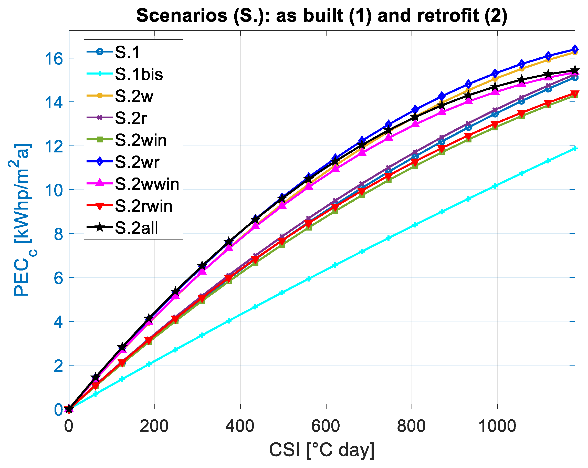
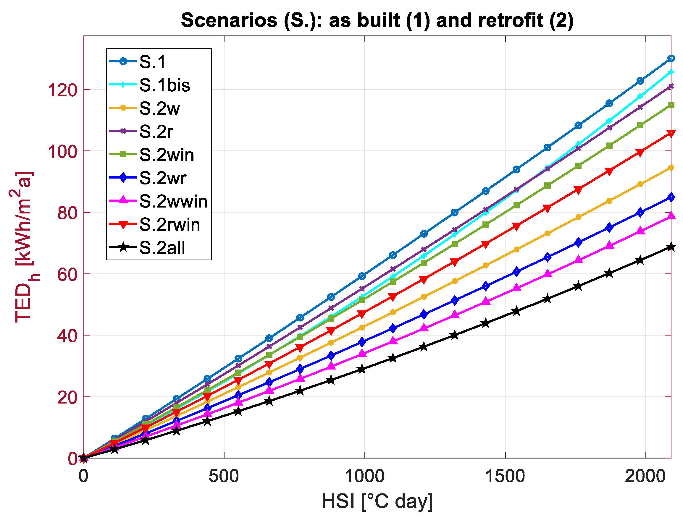
3.2.1. As-Built (S.1) and Retrofit (S.2) Scenarios: A Focus on TED

Figure 7 shows the TED_h as a function of HSI for all investigated scenarios, i.e., the as-built scenario and eight retrofit ones, reporting the average values of all 200 buildings belonging to the RBS. The heating demand is greater in S.1 (as-built) since no energy retrofit measures are implemented. On the other hand, the application of all the retrofit measures (S.2all scenario) can provide the lowest thermal energy demand for heating. Moreover, the difference between the as-built scenario and the others is more visible going toward colder climatic locations because the incidence of different retrofit scenarios is more meaningful. In addition, considering one single curve between HSI 1700 and 2000 °C days, a significant change in the TED_h trend is evident. This occurs because, in this range, the annual rain rate is about half compared to the surroundings (≈600 mm with respect to ≈1000 mm) and the yearly average values of solar radiation are slightly greater (≈200 W/m² with respect to ≈150 W/m²). This results in a local minimum of TED_h.

Considering the different scenarios, the results of the 2nd-order polynomial regression analysis are depicted in Figure 8, providing climatic stress curves that can be used as prediction tools to estimate the average thermal energy demand of the RBS for the different scenarios, thereby enabling the assessment of energy retrofit potentials.

The same approach is applied to TED_c as a function of CSI, as shown in Figure 9. The TED_c should be correlated to CSI and not to HSI since the latter is calculated considering the heating season and not the cooling season. It is evident that the TED_c results are arranged in three main groups: the first, with the greatest values, is composed of S.2all, S.2wwin, S.2wr and S.2w; the second, with medium values, is composed of S.2rwin, S.2win, S.2r and S.1; and the third, with the lowest values, is the S.1bis scenario. This means that:

• on average, not all retrofit measures can cause a reduction in TED_c because they are mainly focused on the improvement of envelope performance in the heating season without considering dynamic parameters such as thermal inertia;
• the group with the highest TED_c values leads to an increase in cooling demand with respect to the as-built scenario since it describes the behavior of a thermally insulated building less able to release the thermal energy stored due to solar and internal gains;
• in particular, the thermal insulation of the building envelope can cause a significant increase in TED_c because of the phenomenon of summer overheating, which can be critical in thermally insulated buildings;
• among all scenarios, the greatest energy savings can be achieved by increasing the cooling set-point temperature, thereby acting on the cooling system management, even if thermal comfort is clearly penalized (S.1bis).

The resulting regression climatic stress curves, which provide the average values of TED_c as a function of CSI for all scenarios, are shown in Figure 10. In this case, the three main groups of results are even more evident.

Finally, Figure 11 represents the average values of TED (TED_c + TED_h) as a function of the YCSI for all scenarios. These curves have similar behavior as the ones related to TED_h vs. HSI because TED_h is predominant with respect to TED_c in the total space conditioning demand. The best solution is once again the one that provides all the retrofit measures (S.2all). Figure 12 shows the related regression climatic stress curves found.

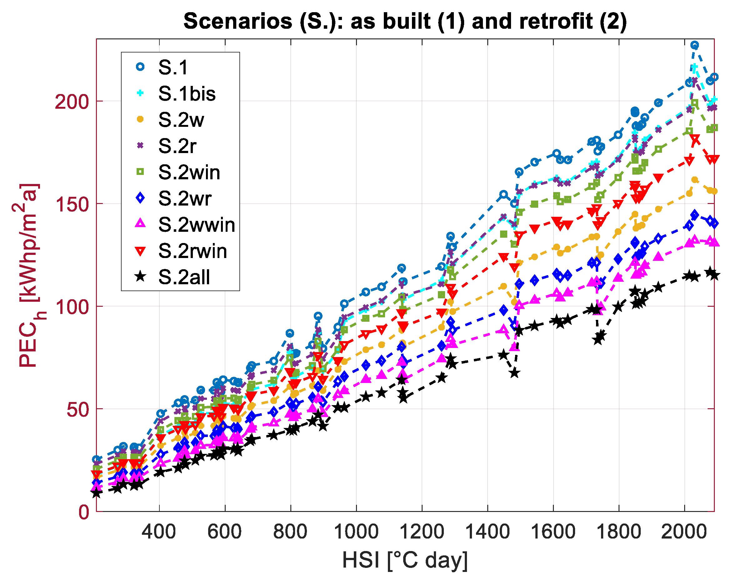
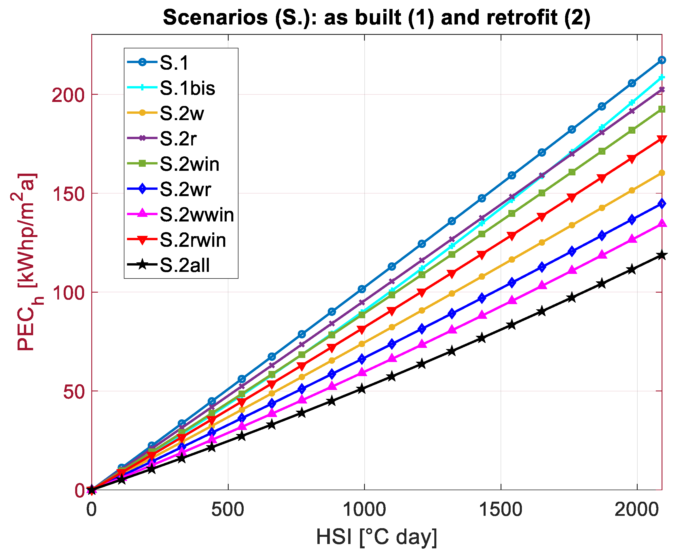
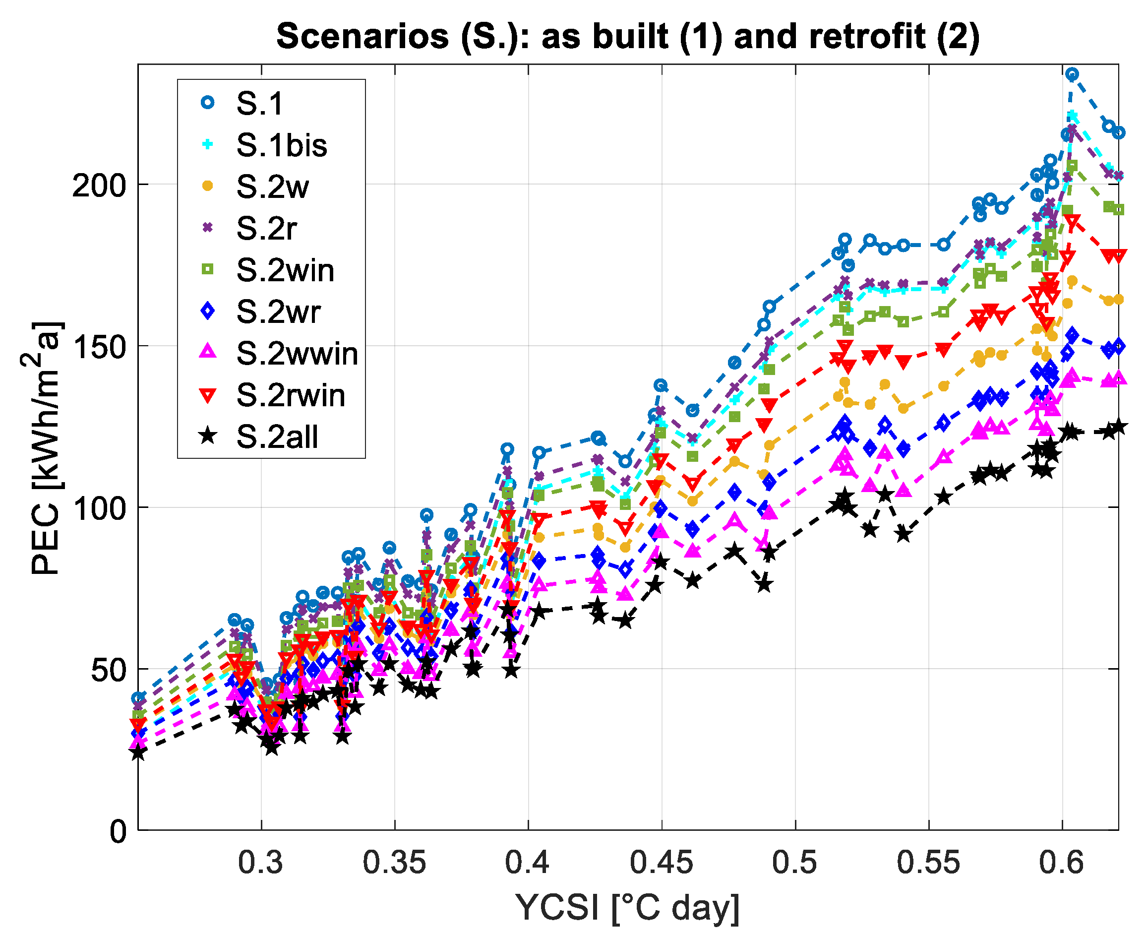
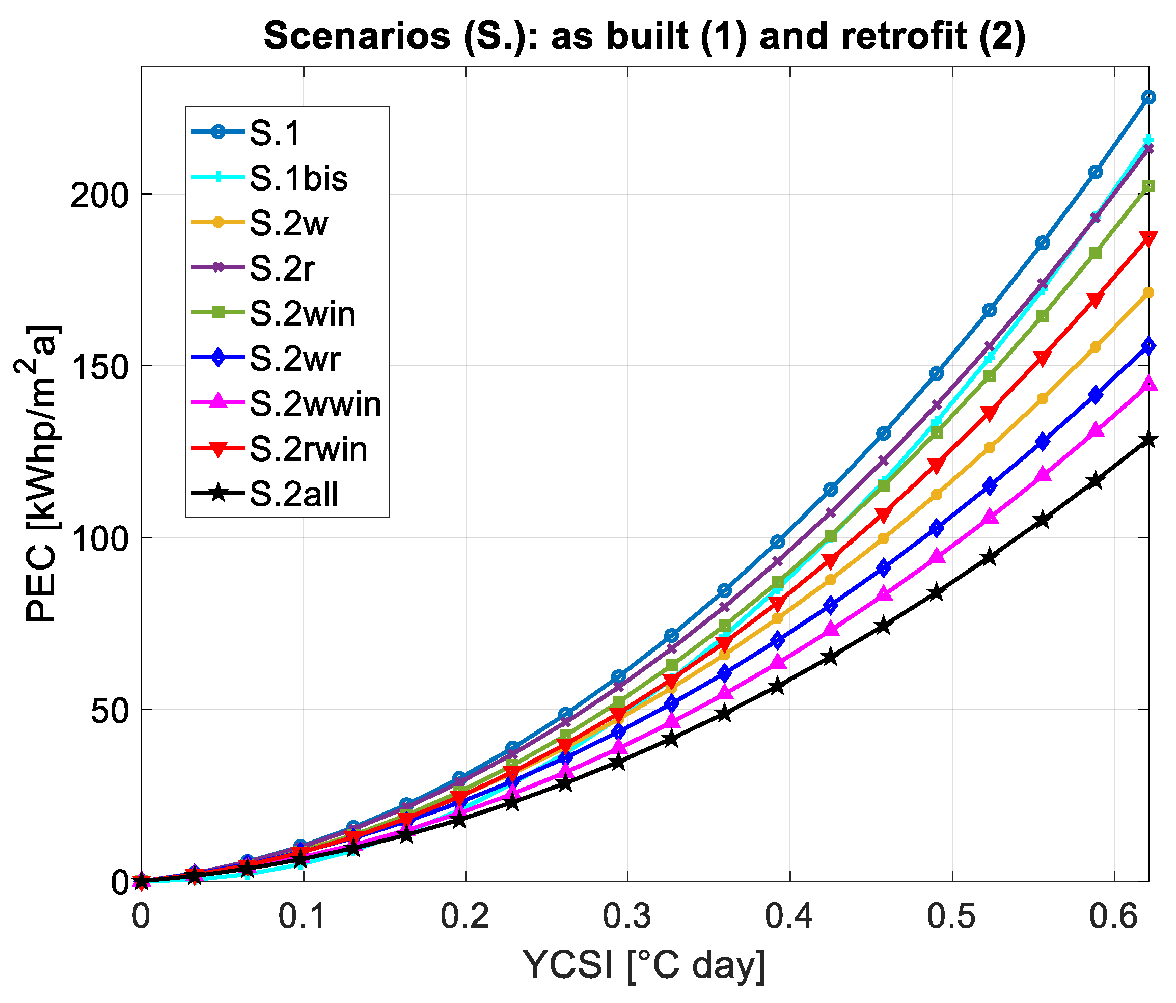
3.2.2. As-Built (S.1) and Retrofit (S.2) Scenarios: A Focus on PEC

The PEC—primary energy consumption—is a useful parameter for choosing the best retrofit measure to be carried out because it is an index of global energy performance considering the whole building’s HVAC system. In particular, the primary energy consumption for heating, PEC_h, is obtained considering the natural gas consumption for heating, with a lower calorific value of 9.59 kWh/Sm³. The primary energy consumption for cooling, PEC_c, considers the average electricity consumption for cooling and the primary conversion factor equal to 1.95 according to Italian law in force [16]. Then, the total PEC is the sum of PEC_h and PEC_c.

The results are shown in Figure 13 and Figure 14 as regards PEC_h, in Figure 15 and Figure 16 as regards PEC_c, in Figure 17 and Figure 18 as regards PEC. Notably, in Figure 13, Figure 15 and Figure 17, there are the relations between PEC_h, PEC_c, PEC and HSI, CSI, and YCSI, respectively, while in Figure 14, Figure 16 and Figure 18, the related regression climatic stress curves are reported. The trends are similar to those related to thermal energy demand, i.e., TED. However, such curves can enable a more comprehensive energy and economic analysis of the retrofit scenarios because they include the performance of the HVAC system.

Notably, the sequential order of the curves related to different scenarios is the same for thermal energy demand and primary energy consumption, respectively, given that these performance indicators are correlated. This shows that the retrofit solutions have the same intervention priority when considering TED or PEC. They are both expressions of how “energy-expensive” it is for the building to deal with the climatic stress, both in terms of thermal energy demand and consumption of primary resources. In other words, the simulation of the HVAC system—passing from thermal energy to primary energy—does not alter the priority ranking of the retrofit solutions.

The economic aspect is neglected in this paper because, currently, the specific prices of energy—i.e., electricity and natural gas prices—are deeply uncertain and volatile in Italy, in Europe and in the whole world because of different reasons, such as the Ukraine–Russia war as well as the public incentives to support energy transition and de-carbonization. However, the proposed climatic stress curves can also be used to predict the running costs for building heating, cooling and total space conditioning by “converting” the primary energy consumption into running costs using the proper specific costs of energy, which depend on location, period and tariff scheme. Thus, economic climatic stress curves—as performed in [21]—can be achieved, providing a precious tool to predict building costs as well as the cost-effectiveness of retrofit scenarios.

Finally, it is highlighted that the proposed approach can take climate change into account because the climatic indices associated with each location can vary according to the actual current weather conditions. In other words, different values of the climatic indices can be associated with the same location. Indeed, the effects of climate change for a given location can be assessed by simply changing the climatic index (i.e., HSI, CSI or YCSI), i.e., the abscissa, for that location when using the proposed climatic stress curves for prediction.

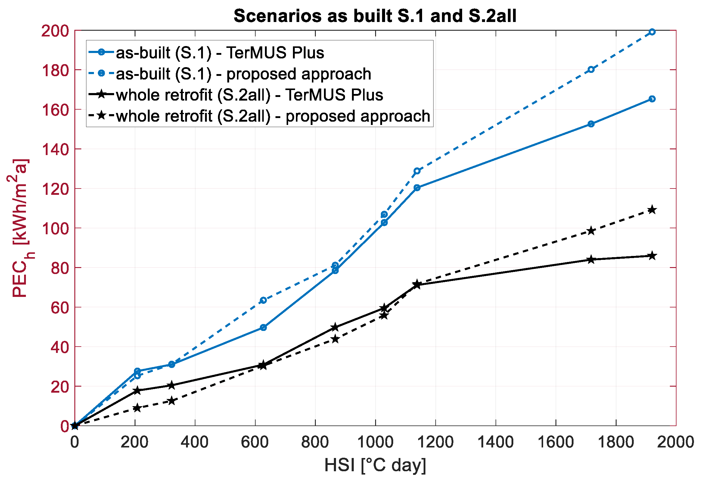
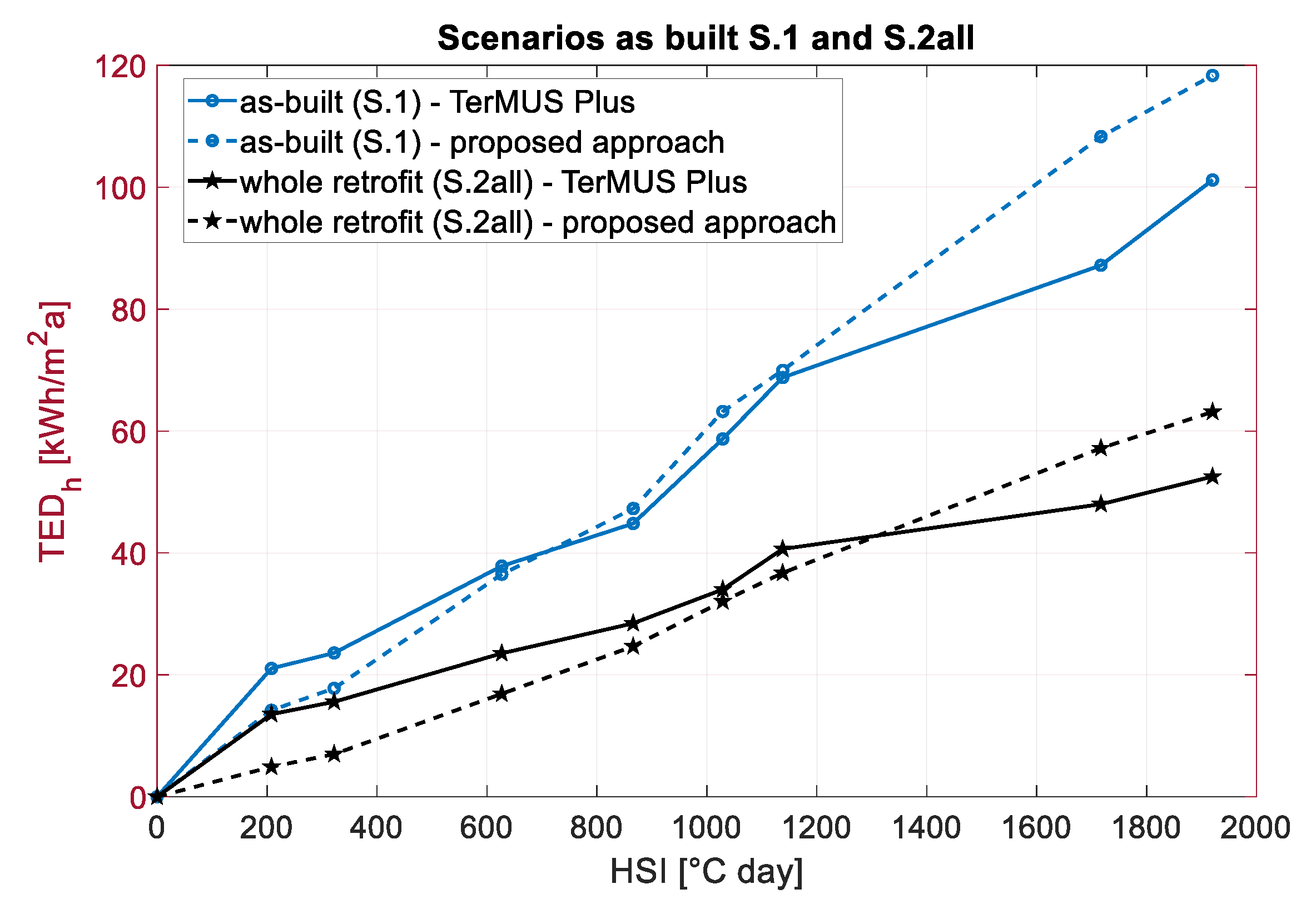
3.3. Testing of the New Approach for an Existing Building Not Belonging to the RBS

In this section, a comparison between the new methodological approach developed to predict TED_h and PEC_h from the HSI and the results deriving from the dynamic energy simulations—using the software TerMUS Plus^® v.1—of an existing building is proposed. For example, only the TED_h and the PEC_h are investigated for the thermal predictions of the building. The building is simulated in various Italian locations, corresponding to the climatic zones from B to E, both in the as-built scenario and in the different retrofit scenarios, as detailed in Section 2.4, where the case study is delineated.

The predictions of the novel approach, which uses the climatic stress curves shown in the previous subsection, refer to the average values in the RBS. Clearly, this is a limitation of this study, which will be addressed in future works.

The results are compared in Figure 19 and Figure 20 as they concern TED_h and PEC_h, respectively. For clarity and brevity, the figures refer only to the as-built (S.1) and whole retrofit (S2.all) scenarios, although all nine scenarios have been simulated.

The curves for the case study achieved via TerMUS^® Plus have similar trends to the ones obtained via the novel approach, related to the average in the RBS. In addition, the sequential order of the scenario curves is the same, yielding the same priority ranking of the retrofit measures.

The EnergyPlus and TerMUS Plus^® simulations provide hourly data for performing dynamic simulations, while the climatic stress curves provide yearly data as concerns thermal and primary energy demands for heating, cooling and space conditioning, respectively. Thus, the testing of the climatic stress curves is performed considering yearly outputs.

In order to perform a more accurate comparison, three error indicators, i.e., the cv(RMSE), the MAPE (mean absolute percentage error) and the MBE (mean bias error), have been assessed for each scenario to evaluate the goodness of the proposed prediction curves. The formula of cv(RMSE) is the one in Equation (7); the formulas of MAPE and MBE are the ones reported in Equations (9) and (10). More specifically, these error indices for the TED_h and PEC_h are evaluated between the average values of the RBS (y_i), which are the predicted outputs, and the actual outputs of TerMUS^® Plus simulations (x_i). The results are shown in

Table 4. Error indicators, i.e., cv(RMSE), MAPE and MBE, were achieved for the testing case study between TerMUS Plus^® and the Novel approach proposed (climatic stress curves).

Scenario	cv(RMSE)		MAPE		MBE
	TEDh	PECh	TEDh	PECh	TEDh	PECh
S.1	17.3%	16.3%	12.7%	11.4%	−4.0 kWh/m2a	−11.0 kWh/m2a
S.2w	27.9%	28.0%	20.3%	20.1%	−5.9 kWh/m2a	−14.1 kWh/m2a
S.2r	15.3%	14.1%	11.5%	9.10%	−2.1 kWh/m2a	−7.7 kWh/m2a
S.2win	18.2%	15.9%	14.5%	10.9%	−0.5 kWh/m2a	−5.3 kWh/m2a
S.2wr	23.2%	23.1%	17.0%	16.3%	−3.2 kWh/m2a	−9.6 kWh/m2a
S.2wwin	26.1%	24.8%	20.2%	17.2%	−1.0 kWh/m2a	−6.2 kWh/m2a
S.2rwin	16.2%	12.1%	15.1%	10.0%	2.3 kWh/m2a	−0.4 kWh/m2a
S.2all	24.0%	20.1%	22.0%	15.1%	1.7 kWh/m2a	−1.5 kWh/m2a

.

$$MAPE=\frac{1}{N}·{\displaystyle \sum }_{i=1}^N\left|\frac{x_i-y_i}{x_i}\right|$$

(9)

$$MBE=\frac{1}{N}·{\displaystyle \sum }_{i=1}^N\left(x_i-y_i\right)$$

(10)

First of all, there is no significant difference in the errors between one scenario and another, thus showing a certain reliability of all curves developed. The error indicators for PEC_h are slightly lower than for TED_h in each scenario. This means that the consideration of primary energy results in fewer errors in predicting performance. Thus, considering PEC_h, the cv(RMSE) varies between 12% and 28%. The MAPE values are 2–8 percentage points lower than the cv(RMSE) results. The MBE for PEC_h varies between −14 and −0.4 kWh/m²a, showing that the climatic stress curves provide an overestimation of primary energy consumption in all scenarios. The MBE for TED_h assumes both negative and positive values, generally close to zero, showing that the curves provide a very good prediction of average thermal energy demand.

Finally, the error indicators may be judged acceptable in regards to the simple model defined and carried out; moreover, the testing case study does not belong to the building sample used for the generation of the climatic stress curves. Indeed, the aim of this study is to provide a very fast and user-friendly tool for an approximate prediction of energy demand for building space conditioning that can support building professionals, designers and policymakers. Note that a limit value of 15%—close to the ones achieved—for cv(RMSE) is defined by ASHRAE Guideline 14 [36] for calibrating a numerical building performance model. On the other hand, also considering the MAPE index, the results are promising because, according to Swanson [37], values lower than 25% indicate acceptable accuracy. Definitely, the proposed approach needs to be improved in terms of reliability and flexibility. Indeed, currently, the curves consider average values in the whole building stock and cannot be particularized for a specific building to achieve higher reliability and accuracy in predictions. In addition, further development to improve the representability of the building stock could be implemented by introducing new variables that consider mechanical ventilation and its operation mode and controls [38].

4. Conclusions

This study aims to define new climatic stress indices and curves to achieve a fast and user-friendly prediction of building energy demands as a function of climatic stress. It focuses on the Italian building stock, but the approach could be applicable to other geographical areas.

By means of the SLABE methodology, by varying building characteristics, 200 theoretically representative buildings are investigated considering 63 climatic locations covering the whole Italian territory. The main results can be summarized as follows:

• The classical approach of DDs (degree days) is not completely reliable to predict building energy needs since solar radiation is not considered. Thus, new climatic stress indices are introduced: the heating stress index (HSI), the cooling stress index (CSI) and the yearly climatic stress index (YCSI), which are determined considering the sol–air temperature. For the HSI and CSI expressions, the decision variables are as follows: T_b (base temperature for DD assessment), T_winter or T_summer, respectively (i.e., the temperatures for the starting of the heating and cooling seasons), and the order of the polynomial in the regression with TED_h and TED_c. The aim is to maximize the coefficient of determination R² between EnergyPlus results and the predictions of the climatic stress curves. This optimization is carried out using brute-force search by varying the integer variables in defined ranges. Two expressions of YCSI are evaluated as functions of HSI and CSI. The optimal results provide regressions of the 2nd order. HSI is characterized by T_b and T_winter both equal to 17 °C, CSI by T_b equal to 22 °C and T_summer equal to 19 °C. The best YCSI expression is as follows:

$$YCSI=0.75*\frac{HSI}{HS{I}_{MAX}}+0.25*\frac{CSI}{CS{I}_{MAX}}.$$

• This result is an evolution of what was achieved in [21], where only the heating stress index was considered. The YCSI is a novelty in the state of the art.
• The climatic stress curves describe the building stock for 63 Italian climatic locations in the as-built scenario and in eight retrofit scenarios. For these curves, the determination coefficient (R²) results are very close to one, thus defining a quite reliable tool to predict thermal energy demand and primary energy consumption. A similar approach to investigating representative building clusters has been developed in [20], which, however, does not refer to the residential sector and does not provide climatic stress curves.
• To evaluate the goodness of the novel approach, an existing building whose energy performance is simulated with another software, i.e., TerMUS Plus^® v.1, is investigated. Thus, a comparison between the novel approach and TerMUS Plus^® v.1 is performed. The cv(RMSE) as well as the MAPE (mean absolute percentage error) assume acceptable values (lower than 28% and 22%, respectively) according to [36,37], considering the simple model defined and the fact that the testing case study does not belong to the RBS used to generate the climatic stress curves.
• The climatic stress curves can also be used to assess the energy efficiency and cost-effectiveness of retrofit solutions as well as their resilience to climate change.

Future studies will focus on enhancing the methodology to parameterize the climatic stress curves as a function of building characteristics, e.g., geometry, envelope, operation and energy systems, with the purpose of obtaining a more reliable tool that can fit different buildings and provide specific curves for each building. Machine/deep learning can be used in this regard, e.g., artificial neural networks.

References

- United Nations Environment Programme. 2021 Global Status Report for Buildings and Construction: Towards a Zero-Emission, Efficient and Resilient Buildings and Construction Sector (Nairobi); United Nations Environment Programme: Nairobi, Kenya, 2021. [Google Scholar]
- United Nations Department of Economic and Social Affairs, Population Division. World Population Prospects 2022: Summary of Results; UNDESA: New York, NY, USA, 2022; Available online: https://www.odyssee-mure.eu/publications/policy-brief/buildings-energy-efficiency-trends.pdf (accessed on 6 June 2023).
- Rousselot, M.; Pinto Da Rocha, F. Energy Efficiency Trends in Buildings in the EU, Policy Brief June 2021. ODYSSEE-MURE Proj. 2021. Available online: http://www.odysseeindicators.org/publications/PDF/Buildings-brochure-2012 (accessed on 6 June 2023).
- Ascione, F.; De Masi, R.F.; Mastellone, M.; Ruggiero, S.; Vanoli, G.P. Improving the building stock sustainability in European Countries: A focus on the Italian case. J. Clean. Prod. 2022, 365, 132699. [Google Scholar] [CrossRef]
- Population Housing Census. Available online: http://dati-censimentopopolazione.istat.it/Index.aspx?lang=en&SubSessionId=9d62b83e-75a2-43a0-abc4-372728b3ed25&themetreeid=16 (accessed on 22 May 2023).
- EU Directive 2018/844 of the European Parliament and of the Council of 30 May. Available online: https://eur-lex.europa.eu/legal-content/IT/TXT/?uri=CELEX%3A32018L0844 (accessed on 22 May 2023).
- IEA. Energy Efficiency 2018: Analysis and Outlooks to 2040; IEA: Paris, France, 2018. [Google Scholar] [CrossRef]
- Makhmalbaf, A.; Srivastava, V.; Wang, N. Simulation-based weather normalization approach to study the impact of weather on energy use of buildings in the US. In Proceedings of the 13th Conference of International Building Performance Simulation Association, Chambery, France, 26–28 August 2013; pp. 1436–1444. [Google Scholar]
- Butche, K. Degree-Days: Theory and Application; The Chartered Institution of Building Services Engineers, CIBSE: London, UK, 2006. [Google Scholar]
- Walsh, A.; Cóstola, D.; Labaki, L.C. Validation of the climatic zoning defined by ASHRAE standard 169-2013. Energy Policy 2019, 135, 111016. [Google Scholar] [CrossRef]
- De Rosa, M.; Bianco, V.; Scarpa, F.; Tagliafico, L.A. Heating and cooling building energy demand evaluation; a simplified model and a modified degree days approach. Appl. Energy 2014, 128, 217–229. [Google Scholar] [CrossRef]
- Kohler, M.; Blond, N.; Clappier, A. A city scale degree-day method to assess building space heating energy demands in Strasbourg Eurometropolis (France). Appl. Energy 2016, 184, 40–54. [Google Scholar] [CrossRef]
- Christenson, M.; Manz, H.; Gyalistras, D. Climate warming impact on degree-days and building energy demand in Switzerland. Energy Convers. Manag. 2006, 47, 671–686. [Google Scholar] [CrossRef]
- Park, J.S.; Sohn, J.Y.; Lee, S.M.; Sung, M.K. Prediction of indoor sol-air temperature in an atrium space with a vertical distribution. In Proceedings of the Healthy Buildings 7th International Conference, Singapore, 7–11 December 2003; National University of Singapore: Singapore, 2003. [Google Scholar]
- Salmerón, J.M.; Álvarez, S.; Molina, J.L.; Ruiz, A.; Sánchez, F.J. Tightening the energy consumptions of buildings depending on their typology and on Climate Severity Indexes. Energy Build. 2013, 58, 372–377. [Google Scholar] [CrossRef]
- Ciulla, G.; D’Amico, A. Building energy performance forecasting: A multiple linear regression approach. Appl. Energy 2019, 253, 113500. [Google Scholar] [CrossRef]
- Neto, A.H.; Fiorelli, F.A.S. Comparison between detailed model simulation and artificial neural network for forecasting building energy consumption. Energy Build. 2008, 40, 2169–2176. [Google Scholar] [CrossRef]
- Andric, I.; Al-Ghamdi, S.G. Climate change implications for environmental performance of residential building energy use: The case of Qatar. Energy Rep. 2020, 6, 587–592. [Google Scholar] [CrossRef]
- Mazzaferro, L.; Machado, R.M.; Melo, A.P.; Lamberts, R. Do we need building performance data to propose a climatic zoning for building energy efficiency regulations? Energy Build. 2020, 225, 110303. [Google Scholar] [CrossRef]
- Mauro, G.M.; Hamdy, M.; Vanoli, G.P.; Bianco, N.; Hensen, J.L. A new methodology for investigating the cost-optimality of energy retrofitting a building category. Energy Build. 2015, 107, 456–478. [Google Scholar] [CrossRef]
- Ascione, F.; Bianco, N.; Mauro, G.M.; Napolitano, D.F.; Vanoli, G.P. Building heating demand vs climate: Deep insights to achieve a novel heating stress index and climatic stress curves. J. Clean. Prod. 2021, 296, 126616. [Google Scholar] [CrossRef]
- DECRETO 26 Giugno 2015. Applicazione Delle Metodologie di Calcolo Delle Prestazioni Energetiche e Definizione Delle Prescrizioni e Dei Requisiti Minimi Degli Edifici; Ministero Dello Sviluppo Economic: Rome, Italy, 2015. (In Italian)
- Decreto del Presidente Della Repubblica 26 Agosto 1993, n. 412. (In Italian). Available online: http://www.decaaced.eu/download/normative/Normative%20Stanziale/DPR%20412%2026%20agosto%201993.pdf (accessed on 1 June 2023).
- UNI 10349-3:2016; UNI Ente Italiano di Normazione—Riscaldamento e Raffrescamento Degli Edifici—Dati Climatici—Parte 3: Differenze di Temperatura Cumulate (Gradi Giorno) ed Altri Indici Sintetici. UNI: Cedar Falls, IA, USA, 2016. (In Italian)
- D.P.R. 1052/1977; Regolamento di Esecuzione Alla Legge 30 Aprile 1976, n. 373, Relativa al Consumo Energetico per Usi Termici Negli Edifici. UNI Ente Italiano di Normazione: Milan, Italy, 1977. (In Italian)
- UNI 6946/2018; UNI Ente Italiano di Normazione—Componenti ed Elementi per Edilizia—Resistenza Termica e Trasmittanza Termica. Metodi di Calcolo: Rome, Italy, 2018. (In Italian)
- UNI 7357/1974; UNI Ente Italiano di Normazione—Calcolo del Fabbisogno Termico Per il Riscaldamento di Edifici. UNI: Cedar Falls, IA, USA, 1974. (In Italian)
- Erbs, D.G.; Klein, S.A.; Beckman, W.A. Sol-air heating and cooling degree-days. Sol. Energy 1984, 33, 605–612. [Google Scholar] [CrossRef]
- Ascione, F.; Bianco, N.; Iovane, T.; Mastellone, M.; Mauro, G.M. Conceptualization, development and validation of EMAR: A user-friendly tool for accurate energy simulations of residential buildings via few numerical inputs. J. Build. Eng. 2021, 44, 102647. [Google Scholar] [CrossRef]
- Ballarini, I.; Corgnati, S.P.; Corrado, V. Use of reference buildings to assess the energy saving potentials of the residential building stock: The experience of TABULA project. Energy Policy 2014, 68, 273–284. [Google Scholar] [CrossRef]
- Corrado, V.; Ballarini, I.; Corgnati, S.P. National Scientific Report on the TABULA Activities in Italy; Dipartimento di Energetica, Gruppo di Ricerca TEBE, Politecnico di Torino: Torino, Italy, 2012; Available online: https://pdfs.semanticscholar.org/fe18/24faf12cc33e9b6135c1416ee33f49a6704e.pdf (accessed on 26 May 2023).
- Canale, L.; De Monaco, M.; Di Pietra, B.; Puglisi, G.; Ficco, G.; Bertini, I.; Dell’Isola, M. Estimating the smart readiness indicator in the italian residential building stock in different scenarios. Energies 2021, 14, 6442. [Google Scholar] [CrossRef]
- Carli, R.; Dotoli, M.; Pellegrino, R.; Ranieri, L. Using multi-objective optimization for the integrated energy efficiency improvement of a smart city public buildings’ portfolio. In Proceedings of the 2015 IEEE International Conference on Automation Science and Engineering (CASE), Gothenburg, Sweden, 24–28 August 2015; pp. 21–26. [Google Scholar]
- Mela, K.; Tiainen, T.; Heinisuo, M. Comparative study of multiple criteria decision making methods for building design. Adv. Eng. Inform. 2012, 26, 716–726. [Google Scholar] [CrossRef]
- EnergyPlus Weather Data. Available online: https://energyplus.net/weather (accessed on 26 May 2023).
- ASHRAE. Measurement of Energy, Demand and Water Savings—Guidelines 14; ASHRAE: Atlanta, GA, USA, 2014. [Google Scholar]
- Swanson, D.A. On the relationship among values of the same summary measure of error when used across multiple characteristics at the same point in time: An examination of MALPE and MAPE. Rev. Econ. Financ. 2015, 5. Available online: https://escholarship.org/content/qt1f71t3x9/qt1f71t3x9.pdf (accessed on 1 June 2023).
- Dai, X.; Cheng, S.; Chong, A. Deciphering optimal mixed-mode ventilation in the tropics using reinforcement learning with explainable artificial intelligence. Energy Build. 2023, 278, 112629. [Google Scholar] [CrossRef]