The Impact of Climate Change and Window Parameters on Energy Demand and CO₂ Emissions in a Building with Various Heat Sources

Abstract

This article presents an original study on the impact of climate change and the area of windows A_wi (factor X₁), the thermal transmittance coefficient of windows U_wi (factor X₂), and the coefficient of total solar transmittance factor of the glazing g_gl (factor X₃) on the index of annual usable energy demand for heating EU_H (function Y) of a single-family residential building in the climatic conditions of Bialystok (Poland), which were loaded with an equal gradual increase in average monthly external temperature by Δθ_e,n (factor X₄). Based on the results of the computational experiment, a deterministic mathematical model of this dependence was developed, and the effects of selected factors on the Y function were analyzed for the considered climatic conditions. Moreover, in cases of selected variants, the influence of the energy source on the amount of final energy used and CO₂ emissions was studied. It was found that an increase in the average monthly external temperature reduces the EU_H of the tested building by 8.4% per every 1 °C of increase in Δθ_e,n. The reduction in CO₂ emissions as a result of climate change is visible for systems with low efficiency and high emission factors (wood boiler), while in the case of pro-ecological high-efficiency systems (with a ground-source pump heat) it is inappreciable. Due to the need to decarbonize buildings, knowledge about the impact of the properties of windows, which are the weakest element in terms of heat loss through the building envelope, as well as the type of heat source on heat demand and CO₂ emissions, is very important for engineers and designers when making the correct decisions.

1. Introduction

Taking urgent action to combat climate change is one of the major challenges of our time. Despite the implementation of numerous measures and legislative actions to improve the efficiency of the building stock, the increased demand due to population growth and rising floor space means that buildings are still responsible for approximately 37% of greenhouse gas emissions in European Union (EU) countries [1]. Therefore, further improvement of their energy efficiency is one of the interventions necessary to achieve the climate goals, which are to hold the increase in the global average temperature to well below 2 °C above pre-industrial levels and pursue efforts to limit the temperature increase to 1.5 °C above pre-industrial levels [2].

The impact of global warming is transforming our environment, increasing the frequency and intensity of extreme weather events, as well as leading to a transformation of ecosystems. This has severe consequences on the productivity of Europe’s economy, infrastructure, ability to produce food, public health, biodiversity, and political stability [3]. Climate change also affects infrastructure, e.g., reducing energy demands in buildings and promoting occupants’ health and comfort [4]. The severity of climate impacts differs not only due to climate variations [5], but also differs between geographical settings (e.g., urban/rural/coastal). Therefore, adapting infrastructure usually requires a complex, site-based analysis of different trends and impact patterns [6].

The EU strategy that can lead to achieving net-zero greenhouse gas emissions by 2050 through a socially fair transition in a cost-efficient manner was presented in November 2018 in the document “Clean Planet for All” [3]. To achieve this goal, in December 2019, the European Commission presented the European Green Deal [7], under which it proposed a new EU target of reducing net greenhouse gas emissions by at least 55% by 2030, compared to their 1990 level. In the construction sector, which despite its large role in global warming has a significant potential for GHG mitigation opportunities, as part of the “Fit for 55” package in March 2023, the European Parliament gave a positive opinion on the amendment to the EPBD directive (on the energy performance of buildings), which was prepared in December 2021. With regard to new buildings, it was established that they should be zero-emission from 2028. Existing residential buildings would have to be classified as at least E on their energy performance by 2030, and D by 2033, on a scale going from A to G, the latter corresponding to the 15% of worst-performing buildings in the national stock of a member state. Non-residential and public buildings would have to achieve the same by 2027 and 2030, respectively [8].

Detailed minimum energy performance requirements and the means to achieve them are set at the national level and adapted to the local climate. The validity of this approach is confirmed by the results of scientific papers. A review of the 128 most cited articles from 1979–2019 on the impact of climatic conditions, building construction, parameters, techniques, and construction methods on energy demand was conducted by Verichev et al. [9]. Based on this analysis, they proved that the appropriate design of buildings in different climate zones depends on a thorough understanding of all climate-dependent aspects, which is also a limiting factor in the development of globally standardized techniques and methodologies. Similar conclusions were presented by Belussi et al. [10]. They reviewed the performance of “zero-energy buildings” and analyzed the impact of the solutions used on energy efficiency. They pointed out that climatic conditions, which vary significantly between and within countries, are the most important geographical factor determining the ability to achieve the expected building standard and influencing the most appropriate technological choices. They indicated that the complexity of simultaneously minimizing energy consumption for heating and cooling, domestic hot water, lighting, and minimizing energy and waste heat production by using low-carbon technologies, and/or utilizing combined heat and power or tri-generation systems varies depending on the geographical context, and it is not possible to determine a single relationship between them. For temperate and especially cold climates (continental or polar [11]), where the demand for space heating in buildings accounts for a significant proportion of the energy consumption, it is crucial to minimize this demand. According to the latest statistical data [12] in Poland (with a cold continental climate [13]), in 2021, space heating accounted for 65.1% of the energy consumed by households. Water heating consumed 17.1% of energy, lighting and electrical appliances (including cooling) 9.2%, and preparing meals 8.3%. Pezzutto et al. [14] estimated that in the EU-15 countries the cooling saturation rate (i.e., share of floor area cooled) is low and in the residential sector it is only 4%. Similar data were presented by Bruno et al. [15], who estimated the share of cooling in residential buildings in EU countries and China at 3%, and only in the United States (US) at 19%. In Poland, in 2021, air-conditioning units were found in only 2.3% of households [12].

One of the main strategies for minimizing energy consumption for heating is limiting the transmission thermal losses through the dispersing elements [15,16], and glazing is the weakest element in terms of heat loss [17]. Valančius et al. [18] compared the thermal transmittance coefficients of windows (U_w) and walls (U_walls) required in recent years in 11 European countries with different climatic conditions (from Nordic to Mediterranean). The strictest requirements for the value of these coefficients apply in countries with colder climates, such as Denmark (U_w = 0.70 W/(m²K) and U_walls = 0.13 W/(m²K)), Norway (U_w = 0.80 W/(m²K) and U_walls = 0.18 W/(m²K)), Lithuania (U_w = 0.90 W/(m²K) and U_walls = 0.13 W/(m²K)), and Finland (U_w = 1.00 W/(m²K) and U_walls = 0.17 W/(m²K)). In each of these countries, the required U_w coefficient was several times higher than U_walls. Less stringent requirements apply in southern and central Europe. In Portugal, in Bragança, U_w = 2.20 W/(m²K) and U_walls = 0.35 W/(m²K); in Lisbon, U_w = 2.80 W/(m²K) and U_walls = 0.50 W/(m²K); and in southern Italy and in Palermo as much as U_w = 3.00 W/(m²K) and U_walls = 0.38 W/(m²K), but in each of these locations the required U-value for windows was several times higher than for walls. In Poland, the requirement U_w = 0.90 W/(m²K) and U_walls = 0.20 W/(m²K) has been in force since 31 December 2020, and is called WT2021 [19]. In the previous periods, they were, respectively: U_w = 1.10 W/(m²K) and U_walls = 0.23 W/(m²K) from 2017 to 2020 (WT2017), and U_w = 1.30 W/(m²K) and U_walls = 0.25 W/(m²K) from 2014 to 2016 (WT2014) [19]. Jezierski et al. [20] studied the impact of changes in the required U-values in force in Poland since 2014 on heating energy demand, heating costs, and emissions. Changing the required U-values of all partitions, excluding the floor on the ground (whose insulation is considered less important), reduced the heating demand of a single-family building by almost 27%, of which windows accounted for 12.8%. Ołtarzewska and Krawczyk [21] analyzed the impact of selected factors on heating costs and air pollution in a cold climate. They considered improvement of the thermal insulation of external partitions, lowering of the indoor temperature in all rooms by 1 °C, moving away from the traditional heat source (gas boiler) to renewable energy (heat pump), and implementation of a heating schedule. The results showed that the most beneficial way to reduce heating costs in the existing service building was to improve the thermal transmittance coefficients of its external partitions and to shorten the heating period. The adoption of these scenarios reduced heating costs by as much as 36% and allowed them to obtain relatively low pollutant emissions. Moreover, replacing the windows alone reduced heating costs by 8%.

It is well known that the heat load varies with the size of the windows (which can be characterized by the window to wall ratio (WWR)) [22] and the nature of this relationship, as in the case of other factors, varies regionally [9,10]. In hot climates, increasing the WWR will significantly increase the cooling load. Kent and Jakubiec [23] conducted research in Singapore, where over half the energy used in buildings is used for cooling, and proved that controlling the size, position, visual lighting technology, and heavily shading windows become crucial to help reduce heat gains, but also to prevent discomfort due to glare. Elghamry and Hassan [24] analyzed the impact of window parameters (shape, construction, size, location, and orientation) on energy consumption, as well as cost, environmental impact (CO₂ emissions), and thermal comfort of a building in hot, semi-arid climatic conditions. They found that controlling the window parameters tested reduces the annual cooling load by approximately 30%, and the lighting power, CO₂ emissions, annual energy consumption, and energy cost by approximately 39%, 22%, 24%, and 21%, respectively. Jezierski and Sadowska [25] optimized three groups of design parameters for a single-family house in a cold continental climate and estimated their contribution to energy saving. The architectural and spatial solutions (building height and window size change factor) had the largest contribution to energy savings (40.0%), factors related to window parameters (thermal transmittance coefficient of windows and total solar transmittance factor) had a slightly smaller share (25.7%), while the smallest contribution was the thickness and density of the material of the internal walls of the building. Kheiri [26] presented a comprehensive review of optimization methods and their application in the architectural design of energy efficient buildings. He considered studies where the building envelope parameters and geometric configurations were the independent variables, and the building’s energy consumption/demand was taken into account as an objective in the optimization process. He emphasized, like other researchers cited earlier [9,10], that determining the best compromises between different shapes of buildings and partition configurations in order to obtain nearly optimal design alternatives in terms of their energy performance is not a simple task.

Energy demand in buildings will also change in response to future climate change, with cooling and heating demand generally moving in opposite directions. Net increases or decreases largely depend on the dominance of cooling or heating demand in a particular region. Overall, global warming will positively impact heating-degree days and negatively influence cooling-degree days. The existing literature discusses changes not only in annual energy consumption for heating, cooling, and other end uses, but also in peak energy consumption, e.g., [27,28,29,30,31,32,33]. There are also studies that reveal the importance of considering future climatic uncertainties when deciding optimal values [34] and selecting building energy retrofit options [35], but climate change is hardly considered at the design stage [36]. Simulations of the performance of buildings and solar energy systems are usually carried out using standard weather files, which generally do not consider future climate forecasts [37].

Future scenarios of global climate change have been presented by the Intergovernmental Panel on Climate Change (IPCC) [38], but it is not certain which scenario will eventually materialize, if any [39]. In order to obtain weather data for use in simulations of the thermal response of buildings that take into account future climate changes, methods of “morphing” weather files have been developed that combine the observed weather data with climate change models [40]. They are used in scientific work for simulations performed with detailed methods. Future climate change scenarios in Poland, where simplified methods of monthly balance sheets are used for the energy assessment of buildings [41], are presented in

Table 1. Changes in selected climate characteristics in Poland by the end of the 21st century (own elaboration based on [32,42]).

Parameter	Period
	1971–1980	1981–1990	1991–2000	2001–2010	2011–2020	2021–2030	2041–2050	2061–2070	2071–2090
Annual average temperature (°C)	7.4	7.8	8.0	8.2	8.6	8.7	9.3	10.1	10.6
No. of days with temperature < 0 °C	114	107	101	102	97	97	82	72	65
No. of days with temperature < 25 °C	27	27	30	29	36	35	37	46	52

.

Since the impact of climate change is regional, this study decided to assess how the energy demand of the building will change while performing a slight renovation of the building [43], including the replacement of windows, in a cold continental climate dominated by heating, for the example of a location in Bialystok (Poland). A single-family house was chosen as a case study, as such houses dominate among residential buildings in Poland [44,45].

The following research questions were formulated: What changes will the increase in average monthly external temperatures, θ_e,n, of the heating period cause? Is it worth looking for new solutions for building windows with further minimization of their thermal transmittance coefficient U_wi? There is no clarity in the selection of the optimal values of the total solar transmittance factor of glazing, g_gl, in the conditions of climate change. In the scientific literature, there are no results of research aimed at estimating the energy effects of climate change, namely, its warming in the aspect of replacing windows. This is an important issue that determines the final energy balance of the entire building, so it should be considered.

Considering the tightened maximum permissible values of heat transfer coefficients of building partition elements in buildings heated for the next period of time, we usually assume that the implementation of these values will result in a uniform reduction in the heat demand for heating for all heated buildings and for all locations, even though they differ significantly in climatic conditions [20,32,46]. However, in the conditions of global warming, the influence of thermal parameters of windows may change with the change of climatic conditions. Unfortunately, to the best knowledge of the authors, there is no data on this subject in the available publications from recent years. The results can be useful both for designers of new buildings and for thermal modernization of existing buildings, when making decisions regarding the selection of window parameters, including changing their area.

Therefore, the purpose of this paper is to study the index of the annual usable energy demand for heating, EU_H, of a selected single-family residential building located in the climatic conditions of Bialystok, depending on the area of the windows A_wi (factor X₁), the thermal transmittance coefficient of the windows U_wi (factor X₂), the total solar transmittance factor g_gl (factor X₃), and the degree of increase in average monthly external temperatures during the heating period Δθ_e,n (factor X₄). Based on the results of the computational experiment, a deterministic mathematical model of this dependence was developed and the effects of the influence of selected factors on the Y function for the assumed conditions were analyzed. Additionally, the discrepancy between the final energy consumption for heating and CO₂ emission in selected scenarios was analyzed.

2. Materials and Methods

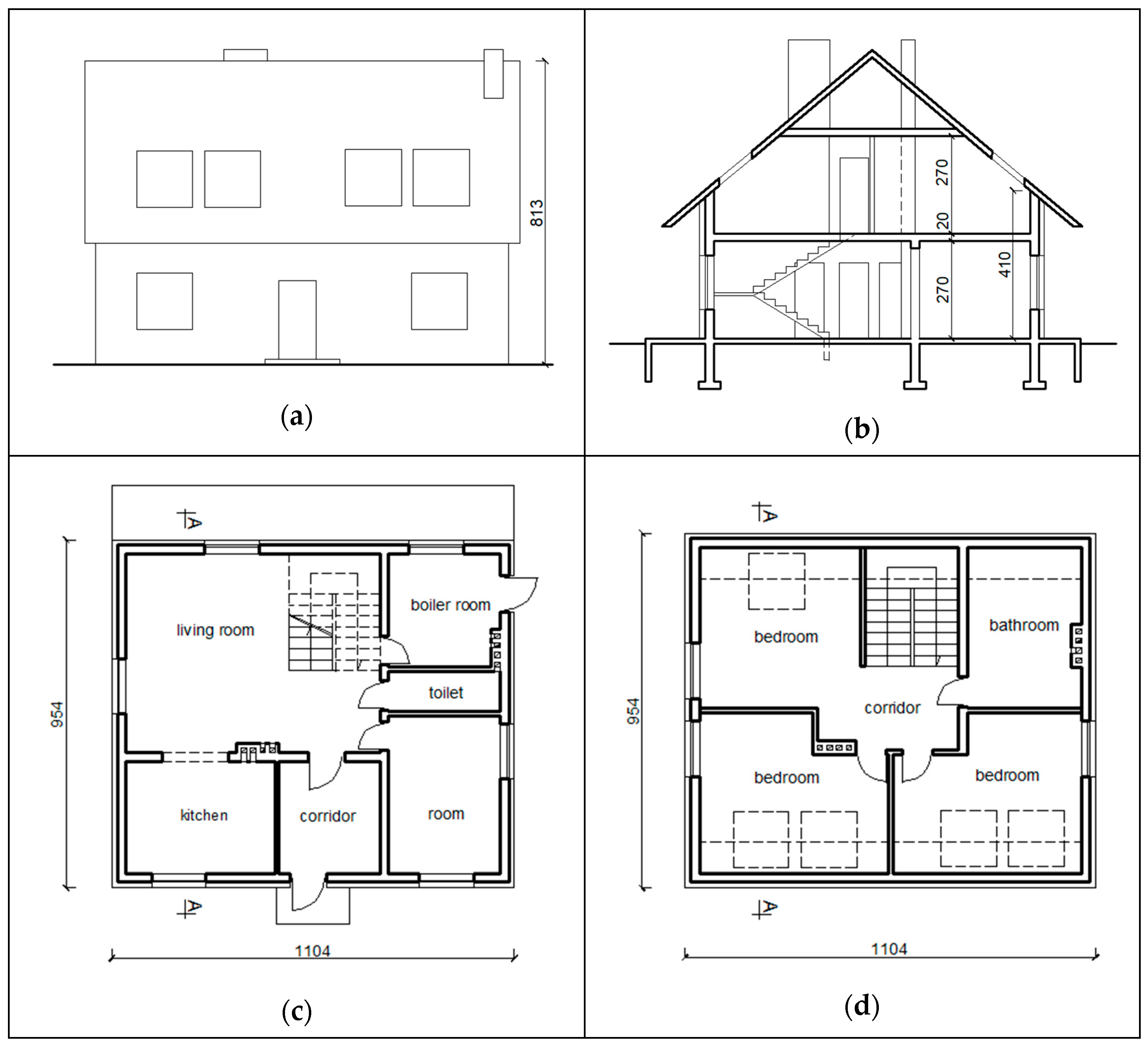
2.1. Characteristics of the Selected Residential Building

A one-story house with an attic was analyzed. It has no basement and was designed in a traditional style, thus, with a simple shape, as an example of a typical single-family house in Poland [43] and the Podlaskie Voivodeship. The building has a rectangular shape with dimensions of 9.54 m × 11.04 m. It was designed in 2019 in traditional brick technology, with a gable roof (an angle of inclination of 45°) and a wooden structure covered with ceramic tiles. The scheme of the analyzed building is shown in Figure 1.

The gross covered area of the building is 105.32 m², the total area is 162.48 m², the usable area is 150.11 m², and the volume is equal to 690 m³. Footings were planned as reinforced concrete and foundation walls of concrete blocks. External walls were designed to be cellular concrete 24 cm thick with a layer of polystyrene on the outside; and the ceiling above the ground floor to be from reinforced concrete. Roof insulation was planned to be made of mineral wool, and plasterboards from the attic side. The floor on the ground consists of the following layers: 10 cm on a gravel bed, roofing felt, polystyrene, and 10 cm thick PE foil floor layers on a concrete base. PVC windows and external doors were planed be used. The thermal transmittance coefficients of individual building envelopes are presented in

Table 2. Thermal transmittance coefficient (U-value) for the analyzed building.

Type of Building Envelope	U-Value
	For the Analyzed Building	In Period of Validity [19]
		2017–2020	Since 31 December 2020
	(W/m2K)
External Walls	0.23	0.23	0.20
Roof	0.18	0.18	0.15
Ground Floor	0.30	0.30	0.30
Door	1.50	1.50	1.30
Windows	0.50; 0.80; 1.10	1.10; 1.30 (for roof windows)	0.90; 1.10 (for roof windows)

. They met the requirements of thermal protection of buildings in Poland [19] during the building design period (2019).

The detailed analysis was conducted for selected energy sources for heating:

• Gas boiler
• Wood boiler
• District heating from Bialystok heat plant
• Ground heat pump (GHP)
• Air heat pump (AHP) combined with a wood fireplace (WF).

A heating, ventilation, and air conditioning (HVAC) system was considered as a water system with plate radiators in the rooms and floor heating in the bathroom; that is the most popular solution in Polish houses. All radiators were equipped with thermostatic valves that have been obligatory in Poland since 1999. Natural ventilation was assumed. Moreover, in line with actual technical conditions, the boilers and district heating supply temperature was set at 70 °C, while for heat pumps it was set at 40 °C. In all cases, automatic control of a heat source based on a heating curve and indoor and outdoor sensors was considered.

It was assumed that the determination of the index of annual usable energy demand for heating, EU_H, of the selected building will be carried out for the climatic conditions of the city of Bialystok (Poland) [47], defined according to the Köppen–Geiger classification [13] as conditions of a temperate continental climate.

Since the analyzed building is not equipped with a cooling system, like the majority (96%) of residential buildings in the EU [12], the demand for cooling was not considered.

2.2. The Method of Calculating the Indicator of the Annual Demand for Usable, Final Energy for Heating and CO₂ Emissions

In this study, in accordance with the adopted objective, the index of annual usable energy demand, EU_H, for heating the building in question was selected as a function of goal Y. This is the quotient of the annual demand for usable energy for heating and ventilation, Q_H,nd, and the heated area, A_f, of the building. The values of Q_H,nd were calculated according to the formulas from the methodology in [41], in force in Poland since 27 February 2015, taking into account the annual demand, Q_H,nd, for each of the s heated zones in the building and for each of the n months of the year. The value Q_H,nd,s,n includes heat losses and gains that shape the energy balance of the building and is determined according to Formulas (1)–(9):

Q_H,nd,s,n = Q_H,ht,s,n − η_H,gn,s,n Q_H,gn,s,n,

(1)

Q_H,ht,s,n = Q_tr,s,n + Q_ve,s,n,

(2)

Q_tr,s,n = H_tr,s (θ_int,s,H − θ_e,n) t_m 10⁻³,

(3)

Q_ve,s,n = H_ve,s (θ_int,s,H − θ_e,n) t_m 10⁻³,

(4)

H_tr,s = ∑ [b_tr,i (A_iU_i + ∑l_iΨ_i)],

(5)

H_ve,s = ρ_ac_a ∑b_ve,s V_ve,s,

(6)

Q_H,gn,s,n = Q_sol,H + Q_int,H,

(7)

Q_sol,H = ∑C_i A_wi I_i F_sh,gl F_sh g_gl,

(8)

Q_int,H = q_int A_f t_m 10⁻³,

(9)

Referring to the presented Formulas (1)–(9) and the methodology in [41], the authors selected four input variables and calculated the index of annual usable energy for heating when changing the values of selected factors according to the calculation experiment plan. The Audytor OZC program was used for the calculations. The block diagram of the method of determining the indicator of the annual demand for usable energy for heating is shown in Figure 2.

Additionally, the total efficiency of the HVAC system was estimated based on the following formula:

η_tot = η_g η_e η_d η,_s,

(10)

The relations between different energy indicators (usable energy, EU, and final energy, EK) are shown in Figure 3.

Transformation of EK to E_CO2 is based on application of the CO₂ emission factor (WE), which in Poland is published annually by the National Center for Energy Balancing and Management [48,49].

2.3. Mathematical Model of the Index of Annual Usable Energy Demand for Heating a Selected Residential Building

Mathematical modeling was used as a research method in this article, which allows us to describe the functioning of the tested object, determine the output parameters, and search for optimal values of the input parameters of the object by means of mathematical dependencies [50]. The use of mathematical modeling allows one to forego physical modeling, shorten the sampling volume, and reduce the labor intensity of the study. The main component in such a system is the mathematical model.

Mathematical models are effective and efficient tools for the analysis of the tested object provided that the developed dependencies are short and the most important factors describing the examined process or property, and having significant meaning for the recipients of information about the tested object, were used in them [50].

As a function of the objective Y, as mentioned above, the index of the annual usable energy demand for heating the tested EU_H of the building was selected, which is a measurable and unambiguous value and has a clear physical sense. The influence of the area of the windows A_wi (factor X₁), the thermal transmittance coefficient of the windows U_wi (factor X₂), the total solar energy transmittance factor of the glazing g_gl (factor X₃), and the degree of increase in average monthly external temperatures Δθ_e,n (factor X₄) were analyzed. The selected factors result from the stated aim of the study. They are measurable, controllable, independent, unambiguous, and non-contradictory, i.e., they meet the basic requirements of mathematical modeling [50].

Other climatic parameters (length of the heating season Ʃt_m and solar radiation in the considered month on the plane in which there is a window I_i) were not included as additional factors in the model, because there is a strong correlation between them, and it does not meet the basic modeling requirements. For this reason, a decision was made to develop and analyze a mathematical model of the above-mentioned dependence on four factors, while only the degree of increase in average monthly outdoor air temperatures throughout the year was selected from the climatic parameters.

It was assumed that the desired dependency Y = f (X₁, X₂, X₃, X₄) could be described by a second-degree polynomial in the form:

Y = a₀ + a₁X₁ + a₂X₂ + a₃X₃ + a₄X₄ + a₁₂X₁X₂ + a₁₃X₁X₃ + a₁₄X₁X₄ + a₂₃X₂X₃ + a₂₄X₂X₄ + a₃₄X₃X₄ + a₁₁X₁² + a₂₂X₂² + a₃₃X₃² + a₄₄X₄²

(11)

To obtain data for the description of this relationship, a four-factor computational experiment was carried out according to the second-stage design. A compositional symmetrical three-level plan containing 24 trials was used [51]. The Audytor OZC program was used to calculate the Y_i value in 24 lines of the plan.

When selecting the range of variation in the X₁ factor, i.e., the area of windows in the selected building (A_wi), at the lower level the value of this factor was adopted as the area of the reference window 1.23 × 1.48 = 1.82 m². The heights of all windows were assumed to be the same and equal to 1.48 m. The subsequent values of the X₁ factor were assumed to be at the level corresponding to the increased window width by 50% and 100% in relation to the reference window, or 1.84 × 1.48 = 2.73 m² and 2.46 × 1.48 = 3.64 m². According to the authors, such a range in variability in the surface of window openings is possible to implement in a residential building and sufficient to detect the effects of this factor. This meets the Polish requirements regarding the minimum window-to-floor ratio of 12.5% [19], as they are 17.0%; 25.4% and 34%. The WWR indexes in these three analyzed cases were 9.16%, 14.35%, and 20.16%, respectively, and only in the first of them it slightly failed to meet the level considered optimal (10–25%) with different types of glazing, as well as with different levels of heat transfer [22].

The X₂ factor, i.e., the value of the thermal transmittance coefficient of windows, was adopted at the basic level of 0.80 W/(m²K). The upper level was declared as 1.10 W/(m²K) in accordance with the upper requirement in Poland for windows during the building design period [19]. This U_wi value characterizes the most frequently used windows in Polish houses (double glazing window with one coated pane with argon gas between panes, insulated window frames, traditional edge spacer). The lower level was set at 0.50 W/(m²K). This has been tightened, as work is underway to implement innovative window solutions with such a thermal transmittance coefficient (triple pane window with low emission surfaces and gas between the panes with better properties than argon, insulated window frames with glass fiber reinforcement, edge spacer with improved thermal properties).

The X₃ factor, i.e., the coefficient of transmittance of the total solar radiation of the glazing, was assumed to be equal to 0.50 at the average level; at the upper level: 0.70; at the lower level: 0.30. It is worth noting that the total solar transmittance factor of the glazing (g_gl) usually correlates with the value of the heat transfer coefficient of the glazing U_g and, in turn, with the value of the U_wi coefficient of the window. However, for research purposes, the authors hypothetically assumed the lack of such a correlation, i.e., the independence of the total solar radiation transmittance coefficient of the glazing from the glazing heat transfer coefficient was assumed. This approach allows the expansion of the space for searching for optimal values of window parameters.

The last factor, X₄, i.e., the degree of increase in average monthly external temperature throughout the year (Δθ_e,n), was also assumed at three levels. At the lower level, the current values of average monthly external temperatures in Bialystok were adopted according to the data of the meteorological station [47] (Δθ_e,n = 0 °C). At the average level, the current values of average monthly outdoor temperatures were increased by 1 °C each month (Δθ_e,n = 1 °C). At the upper level, the current values of average monthly external temperatures were equally increased by 2 °C (Δθ_e,n = 2 °C).

The above-mentioned natural values of the factors Ẋ₁, Ẋ₂, Ẋ₃, Ẋ₄ and the corresponding standardized values (in brackets) of normed values X₁, X₂, X₃, X₄ are presented in

Table 3. Natural and standardized values of selected factors.

Factor Level Ẋi	Awi (m2)	Uwi (W/(m2K))	ggl (-)	Δθe,n (°C)
	(X1)	(X2)	(X3)	(X4)
Bottom (−1)	1.82 (1.23 × 1.48)	0.5	0.3	0.0
Middle (0)	2.73 (1.84 × 1.48)	0.8	0.5	1.0
Upper (+1)	3.64 (2.46 × 1.48)	1.1	0.7	2.0
Range of factor change ΔXi	0.91	0.3	0.2	1.0

. The transition from natural Ẋ_i to normative values X_i [51] is expressed by Formula (12):

X_i = [2Ẋ_i − (Ẋ_imax + Ẋ_imin)]/(Ẋ_imax − Ẋ_imin),

(12)

where Ẋ_i, Ẋ_i,max, and Ẋ_i,min are the current, maximum, and minimum natural values of the i-th factor, respectively.

Other input parameters were assumed to be constant. The geometrical parameters characterizing the shape and area of the rooms, as well as the physical properties of the materials used, are described in Section 2. Climatic conditions were adopted for Bialystok according to [47], on the basis of which the calculated number of days of the heating season is 232 days. The orientation of the front façade of the building was adopted the same for all variants—from the north.

Since the contribution of the glazing area to the total window area C_i depends on the independent variable A_wi (factor X₁), for the selected levels of this factor (Table 3) and the assumed width of the frame elements b_f = 0.10 m, the values of C_i were calculated, which were 0.724 (at A_wi = 1.82 m²), 0.771 (with A_wi = 2.73 m²), and 0.795 (with A_wi = 3.64 m²) (Figure 4). For these values, the dependency function C_i = f(A_oi) was selected, which had the form C_i = 0.040·A_wi + 0.654 and was included in the program for EU_H calculations according to the plan (

Table 4. Planning matrix and calculation results of EU_H (Y_i).

No	X2	X3	X4	X5	EUHI (YI,i)
					(kWh/(m2year))
1	1.82 −1	0.50 −1	0.3 −1	0 −1	81.8
2	3.64 1	0.50 −1	0.3 −1	0 −1	77.2
3	1.82 −1	1.10 1	0.3 −1	0 −1	92.0
4	3.64 1	1.10 1	0.3 −1	0 −1	97.0
5	1.82 −1	0.50 −1	0.7 1	0 −1	69.9
6	3.64 1	0.50 −1	0.7 1	0 −1	59.3
7	1.82 −1	1.10 1	0.7 1	0 −1	79.5
8	3.64 1	1.100 1	0.7 1	0 −1	77.0
9	1.82 −1	0.500 −1	0.3 −1	2 1	68.7
10	3.64 1	0.500 −1	0.3 −1	2 1	64.9
11	1.82 −1	1.100 1	0.3 −1	2 1	77.5
12	3.64 1	1.100 1	0.3 −1	2 1	81.9
13	1.82 −1	0.500 −1	0.7 1	2 1	58.6
14	3.64 1	0.500 −1	0.7 1	2 1	49.2
15	1.82 −1	1.100 1	0.7 1	2 1	66.9
16	3.64 1	1.100 1	0.7 1	2 1	64.6
17	1.82 −1	0.800 0	0.5 0	1 0	73.3
18	3.64 1	0.800 0	0.5 0	1 0	69.8
19	2.73 0	0.500 −1	0.5 0	1 0	64.6
20	2.73 0	1.100 1	0.5 0	1 0	77.9
21	2.73 0	0.800 0	0.3 −1	1 0	76.0
22	2.73 0	0.800 0	0.7 1	1 0	64.5
23	2.73 0	0.800 0	0.5 0	0 −1	75.2
24	2.73 0	0.800 0	0.5 0	2 1	63.2

).

3. Results and Discussion

3.1. Development of Mathematical Models of the Studied Dependencies

Based on the results of EU_H calculations (Table 4) using the least squares method [51] a mathematical model was developed in the form of a regression equation of Y = f(X₁, X₂, X₃, X₄):

Y = 69.79 − 1.52X₁ + 6.67X₂ − 7.08X₃ − 6.30X₄ + 2.06X₁X₂ − 1.61X₁X₃ + 0.10X₁X₄ − 0.30X₂X₃ − 0.49X₂X₄ + 0.54X₃X₄ + 1.76X₁² + 1.46X₂² + 0.46X₃² − 0.59X₄²

(13)

To evaluate the accuracy of the developed deterministic model, the mutually unambiguous correspondence between the external impact and the response to this impact was taken into account. Since only one computational experiment was performed at each point in the plan, there were no repetitions and no variance of measurement inaccuracies. The adequacy of the model [50] could, therefore, be assessed by comparing the variances of the mean S²_y and the residual variance S²_r calculated according to (15) and (16):

S²_y = Σ(Y_i − Ȳ)²/(N − 1),

(14)

S²_r = Σ(Ŷ_i − Y_i)²/(N − N_b),

(15)

Then, the Fisher criterion was calculated [51]:

F = S²_y(f₁)/S²_r(f₂),

(16)

where f₁ = (N − 1) = 24 − 1 = 23 and f₂ = (N − N_b) = 24 − 16 = 9.

This criterion made it possible to detect the degree of reduction in dissemination with respect to the regression equation compared to the average spread [51]. If the value of F is much greater than the value of the F_t from tables, then with the selected significance p and the degrees of freedom f₁ and f₂, it can be concluded that the model is adequate.

Since F = 113.9361/0.5812 = 196.0242 exceeds F_t = F_0.05;23;9 = 2.91 by many times [52], the model is adequate. In addition, its good quality is confirmed by the determination coefficient: R² = 0.9980.

Using the t-criterion, the significance of the coefficients was assessed. According to [52], for each coefficient t_j = |b_j|/S_bj was calculated from the residual variance S_r². This value was compared with the critical value of t_0.05;5 = 2.02 [50]. If t_j < t_0.05;5, the coefficient was considered irrelevant. After assessing the accuracy of the model, it was used for further analysis.

3.2. Analysis of the Examined Dependence on the Basis of a Mathematical Model

The analysis of the influence of the examined factors on the indicator of the annual demand for usable energy for heating the selected building was made on the basis of a mathematical model (13). For better clarity, the results will be discussed using natural variables.

Analyzing the developed model, it was found that in the center, G_p, of the multifactor space, which is characterized by the coordinates corresponding to A_w0 = 2.73 m²; U_w0 = 0.80 W/(m²K); g_gl = 0.5; and Δθ_e,n = 1 °C, the value of the index of annual usable energy demand for heating the building is EU_H = 69.79 kWh/(m²year).

Using the G_p point as a reference point, the impact of individual factors was estimated. According to the obtained model (13), the strongest and most beneficial influence on EU_H is the factor X₃—the total solar transmittance factor of the glazing g_gl. When the g_gl coefficient is changed from 0.30 to 0.70, the EU_H decreases from 77.33 to 63.17 kWh/(m²year), i.e., by 18.3%.

A similar nature and strength of influence was also demonstrated by factor X₄—the degree of increase in average monthly external temperatures throughout the year, Δθe,n. When Δθ_e,n changes from 0 to 2 °C, the EU_H decreases from 75.50 to 62.90 kWh/(m²year), i.e., by 16.7%. Factor X₁—the area of windows, A_w0, has a weak, but also positive effect on EU_H. When A_w0 changes from 1.82 to 3.64 m², the EU_H decreases from 73.07 to 70.03 kWh/(m²year), i.e., by 4.2%.

Only the factor X₂—the thermal transmittance coefficient of windows U_w0, showed a strong adverse effect. When U_w0 changes from 0.50 to 1.10 W/(m²K), EU_H increases from 64.58 to 77.92 kWh/(m²year), i.e., by 20.7%.

The described nature of the influences of the factors is also reflected in Figure 5, which shows the graphical relationship EU_H = f(g_gl, Δθ_e,n) for A_w0 = 2.73 m² and U_w0 = 0.80 W/(m²K).

As can be seen from the presented data, the fluctuations of the considered factors confirm the sensitivity of the examined function, but they give different increases in EU_H. The influence of the factor Δθ_e,n (X₄) was analyzed in the most detail. It was noted that in model (13) there are several weak interaction effects of this factor with the other factors (+0.10X₁X₄; −0.49X₂X₄; +0.54X₃X₄). By analyzing the signs of these effects, it was found that with the increase in the X₄ factor, the effects of the influence of the X₁, X₂, and X₃ factors weakened. At the same time, for two pairs of factors X₁–X₄ and X₃–X₄, it was found that each factor of the pair separately has a stronger effect than when the other factor is affected simultaneously. In order to fully analyze X₄, its impact had to be estimated at the appropriate extreme values of X₁, X₂, and X₃, which result from the previous analysis of individual factors and were limited by the range in variability adopted in the study. After substituting the values of these factors into model (13) and performing simulation calculations, significant information about the degree of influence of the X₄ factor was obtained. The calculation results are presented in

Table 5. Evaluation of the impact of the considered factors on EU_H with climate change (Δθe,n = 0; 1; 2 °C).

Δθe,n (°C)	Awi (m2)	Uwi (W/(m2K))	ggl (-)	EUH
(X4)	(X1)	(X2)	(X3)	kWh/(m2year)
0 (−1)	3.64 (+1)	0.50 (−1)	0.70 (+1)	59.41
	1.82 (−1)	1.10 (+1)	0.30 (−1)	92.21
1 (0)	3.64 (+1)	0.50 (−1)	0.70 (+1)	54.83
	1.82 (−1)	1.10 (+1)	0.30 (−1)	85.37
2 (+1)	3.64 (+1)	0.50 (−1)	0.70 (+1)	49.07
	1.82 (−1)	1.10 (+1)	0.30 (−1)	77.35

.

For a building with windows with deteriorated parameters (A_wo = 1.82 m²; U_wo = 1.10 W/(m²K); g_gl = 0.30), climate changes along with an increase in average monthly external temperatures throughout the year Δθ_e,n from 0 to 2 °C cause a decrease in EU_H from 92.21 to 77.35 kWh/(m²year), i.e., by 16.1%. For a building with windows with improved parameters (A_w = 3.64 m²; U_wo = 0.50 W/(m²K); g_gl = 0.70), an increase in average monthly external temperatures throughout the year from 0 to 2 °C also causes a decrease in EU_H (from 59.41 to 49.07 kWh/(m²year), i.e., by 17.4%). Taking into account a very weak square effect (−0.59 X₄²), it can be concluded that an increase in average monthly external temperatures throughout the year by 2 °C from the current state, for a building with windows with the same parameters, regardless of whether they are good or bad, causes a decrease in EU_H by an average of (16.1 + 17.4)/2 = 16.75%, or 8.4% for every 1 °C.

Then, the significance of the interaction effects of factor X₄ with the other factors was checked. For this purpose, the values X₄ = −1 were substituted into model (13); 0; +1. After the transformation, three equations were obtained, which characterized the relationships EU_H = f(A_w0, U_w0, g_gl) for periods with the current climatic conditions (Δθ_e,n = 0 °C—model (17)); with warming climate in the first stage (Δθ_e,n = 1 °C—model (18)); and with climate change in the second stage (Δθ_e,n = 2 °C—model (19)):

Y₁ = 75.50 − 1.62X₁ + 7.16X₂ − 7.62X₃ + 2.06X₁X₂ − 1.61X₁X₃ − 0.30X₂X₃ + 1.76X₁² + 1.46X₂² + 0.46X₃

(17)

Y₂ = 69.79 − 1.52X₁ + 6.67X₂ − 7.08X₃ + 2.06X₁X₂ − 1.61X₁X₃ − 0.30X₂X₃ + 1.76X₁² + 1.46X₂² + 0.46X₃²

(18)

Y₃ = 62.90 − 1.42X₁ + 6.18X₂ − 6.54X₃ + 2.06X₁X₂ − 1.61X₁X₃ − 0.30X₂X₃ + 1.76X₁² + 1.46X₂² + 0.46X₃²

(19)

Using the developed models (17)–(19), simulation calculations were made (

Table 6. Evaluation of the interaction effects of factor X₄ with factors X₁, X₂, and X₃ in the relationships Y_i = f(X₁,X₂,X₃).

Δθe,n (°C) (X4)	Awi (m2) (X1)		Uwi (W/(m2K)) (X2)		ggl (-) (X3)
	1.82 (−1)	3.64 (+1)	0.50 (−1)	1.10 (+1)	0.30 (−1)	0.70 (+1)
0 (−1)	78.88	75.64	69.80	84.12	83.58	68.34
	−4.1%		20.5%		−18.3%
1 (0)	73.07	70.03	64.58	77.92	77.33	63.17
	−4.2%		20.7%		−18.3%
2 (+1)	66.08	63.24	58.18	70.54	69.90	56.82
	−4.3%		21.2%		−18.7%

) and the nature and degree of the influences of factors X₁, X₂, and X₃ for various levels of climate warming were analyzed.

The change in the value of the analyzed factors changes the EU_H value at each level of climate change to an almost equal degree, namely, X₁ by (−4.1) ÷ (−4.3)%; X₂ by 20.5 ÷ 21.2%; X₃ by (−18.1) ÷ (−18.7)%. This means that the interaction effects of factors detected in the model (13) turned out to be insignificant and an increase in the average monthly external temperatures throughout the year, Δθ_e,n, practically do not change the degree and nature of the impact of the geometric and physical parameters of the windows on the energy performance of the building.

Warming of the climate, which turned out to be one of the most important factors considered in this article, in northern and central Europe reduces the number of days when heating is needed; however, the demand for cooling will certainly increase, which may lead to higher total energy consumption. A similar trend occurs in hot climates. However, since cooling systems are used very rarely in Polish single-family buildings, only energy consumption for heating was analyzed. It is worth noting, however, that climate warming will increase the discomfort of residents in such conditions. Therefore, when designing new buildings or replacing windows in existing buildings, it is worth paying attention to another factor considered in the article, which turned out to be the factor g. Increasing its value from 0.3 to 0.7 had the greatest impact on reducing the demand for heating energy; however, also in the case of cooling, this factor will have a very significant effect. It will also, like the WWR indicator, change how much daylight is admitted into the building and change the lighting load [23]. Therefore, crucial for reducing heat gains is the careful selection of the window type, including the materials they are made of, but also their properties, size and location, shading elements, etc.

The described nature of the impact of the selected factors complements the knowledge about the energy and economic effects in a heated building from changes in the window parameters in the conditions of climate change, expressed only by an increase in average monthly external temperature. However, it is necessary to carry out similar research in the conditions of climate warming with the changes in other climate indicators.

3.3. Analysis of the Impact of the Type of Heat Source on the Amount of Final Energy and CO₂ Emissions of the Considered Building in the Conditions of Climate Change

For the analysis of the energy-consuming level of the tested building, a solution with average parameters of the windows was selected: surface area A₀ = 2.73 m²; heat transfer coefficient U₀ = 0.800 W/(m²K); and coefficient of the total solar radiation transmittance of the glazing g_gl = 0.5. Three climatic scenarios were taken into consideration: S.1., actual conditions (Δθ_e,n = 0 °C); S.2., first-level climate-warming (Δθ_e,n = 1 °C), and S.3. second-level climate-warming (Δθ_e,n = 2 °C). Based on the models described by (13), (14), and (15), the EU_H factors for scenarios 1, 2, and 3 were delivered with EU_H equal to 75.50 kWh/(m²year); 69.79 kWh/(m²year) and 62.90 kWh/(m²year), respectively. Then, the final energy consumption for each scenario was calculated taking into account the total efficiency of each system (Formula 10). The lowest efficiency of the system (0.60) was found in the case of the wood boiler, as the result of having the lowest efficiency of energy generation, while the highest efficiency of the system was supplied from the ground heat pump (3.05). For the HVAC system with an air heat pump and a fireplace, the total efficiency was estimated to be between 0.80 when the AHP share was 25% and 1.51, corresponding with a 75% share in the whole balance. The efficiency of the system with a gas condensing boiler was found to be slightly lower (0.81) than when the building was supplied from the city’s heat plant. The results are presented in

Table 7. EK values for the analyzed scenarios.

Variant	Description	Scenario 0	Scenario 1	Scenario 2
1 (V.1)	Gas boiler	92.93	85.90	77.42
2 (V.2)	Wood boiler	126.24	116.69	105.17
3 (V.3)	District heating from Bialystok heat plant	86.29	79.77	71.89
4 (V.4)	Ground heat pump	24.73	22.86	20.60
5 (V.5)	Air heat pump combined with a wood fireplace	(A) 50.14 * (B) 65.87 * (C) 94.47 *	(A) 46.35 * (B) 60.89 * (C) 87.33 *	(A) 41.77 * (B) 54.88 * (C) 78.71 *

* (A) 25%AHP + 75%WF, (B) 50%AHP + 50%WF, (C) 75%AHP + 25%WF.

.

The results show that the selection of the HVAC system and source has a significant influence on the final energy consumption in the analyzed house, as the variant with the GHP as a source for a low temperature water system results in a five times lower final energy consumption compared to the higher temperature system with the wood boiler. In contrast, differences between scenarios 0–1 and 0–2 are constant (7.5% and 16.7%, respectively) and a result of EK values. Additionally, the energy savings in the wake of climate-warming were estimated. In the case of Scenario 2 happening, the highest reduction in energy consumption appears in the system with the wood boiler (1433.13 kWh), while the lowest is in the case with the GHP (280.71 kWh). Second-level climate-warming (Δθ_e,n = 2 °C) would decrease the energy consumption for heating in the range between 619.44 kWh and 3162.43 kWh, being in each case a 16.7% reduction in Polish climate conditions.

In addition, the CO₂ emissions for each variant and scenario were estimated using emission factors from the ECO-Auditor Sankom software 1.0 Edu PL [53] that align with Polish regulations [54,55,56]. The results are presented in Figure 6.

The most eco-friendly solution is the system with the GHP as the result of low energy consumption and emission factor. The highest CO₂ emission was found in the case of the wood boiler. Comparable results were found for the gas boiler and the system supplied by AHP combined with a wood fireplace. Looking into the reduction in CO₂ emissions after climate warming by 1 °C and 2 °C, a significant effect can be seen in the low efficiency, high temperature HVAC system with the wood boiler that is equal to 221 and 488 g CO₂/year, respectively. This is nearly twice as high as in the system supplied from the GHP (120 and 266 g CO₂/year).

4. Summary and Conclusions

The developed deterministic mathematical model allowed the estimation of the effects of the influence of the selected window parameters on the index of annual usable energy demand for heating, EU_H, in the case of a single-family residential building located in northeastern Poland (city Bialystok) under climate change conditions. The base conditions were assumed to be the actual levels, taking into account the average monthly external temperature, Δθ_e,n, from the Bialystok weather database and the window parameters as described in Section 2.

• It was found that an increase in average monthly external temperature reduces the index of annual usable energy demand for heating, EU_H, of the tested building by about 8.4% for every 1 °C of increase in Δθ_e,n. After taking into account the efficiency of the heating system (considering energy generation, accumulation, regulation, and transfer into heating zones) a final energy consumption indicator was estimated. Scenario 1 (Δθ_e,n = 1 °C) results in the highest savings for the system, with the lowest efficiency system (wood boiler) equal to 1433.13 kWh, while the lowest reduction was found for the high-efficiency system with a ground-source heat pump (280.71 kWh).
• Global warming at the level of 2 °C would lead to an approximately 16.7% reduction in final energy consumption. Depending on the heating system used, the savings would range from 619.44 to 3162.43 kWh.
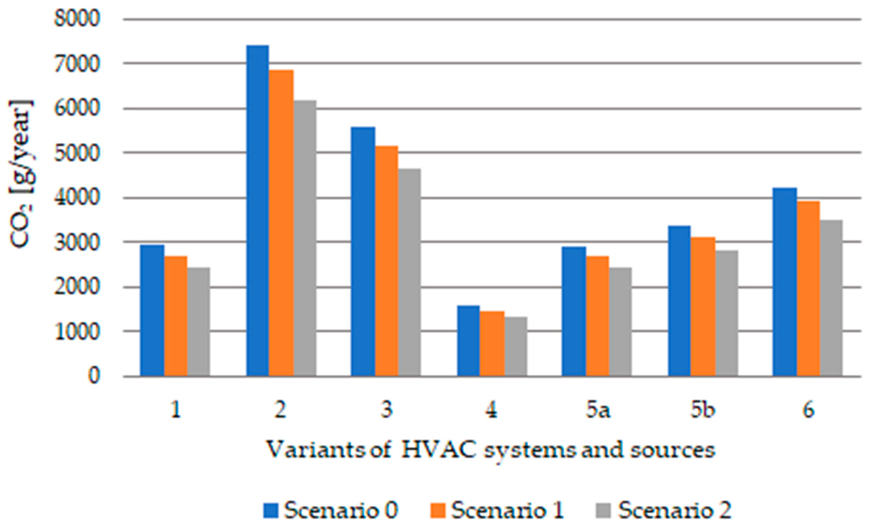
• A reduction in CO₂ emission as the result of climate warming is visible for systems with low efficiency and high emission factors (V.2), while in the case of eco-friendly solutions (such as the GHP in V.4) any reduction is inappreciable.
• It was found that the warming climate, expressed only in terms of an increase in the average monthly external temperature in the individual months of the heating season Δθ_e,n, practically does not change the degree and nature of the influence of selected window parameters on the energy performance of the building. The most significant influence (18.3%) among the analyzed factors is the total solar transmittance factor of glazing g_gl and the degree of increase in average monthly external temperature throughout the year Δθ_e,n (16.7%). In contrast, the effect of the change in window area on EU_H is much smaller, amounting to about 4.2%.

Moreover, it is worth emphasizing that in the climatic conditions of Bialystok, the demand for energy for cooling is negligible (as described in Section 1), hence this issue has not been considered. On the other hand, climate warming may result in a variable impact of window parameters on the energy performance, final energy consumption, and emission of pollutants into the atmosphere in the case of a building located in the south of Europe due to a remote share of heating and cooling in the annual energy balance; this will be the subject of further analysis.

Due to the need to further improve the energy efficiency of buildings, even those with pretty good thermal quality, as part of their decarbonization, knowledge of the impact of the performance of windows (which are the weakest element in terms of heat loss through the building envelope) as well as the type of heat source on the energy demand and resulting CO₂ emissions may be useful for engineers and designers responsible for decision making during the design of new or retrofitting of existing buildings.

References

1. United Nations Environment Programme. 2022 Global Status Report for Buildings and Construction. Towards a Zero-Emission, Efficient and Resilient Buildings and Construction Sector. Nairobi. 2022. Available online: https://www.unep.org/resources/publication/2022-global-status-report-buildings-and-construction (accessed on 29 May 2023).
2. United Nations. Paris Agreement. 2015. Available online: https://unfccc.int/process-and-meetings/the-paris-agreement/the-paris-agreement (accessed on 10 May 2023).
3. European Commission. A Clean Planet for All. A European Strategic Long-Term Vision for a Prosperous, Modern, Competitive and Climate Neutral Economy. 2018. Available online: https://eur-lex.europa.eu/legal-content/EN/TXT/PDF/?uri=CELEX:52018DC0773&from=EN (accessed on 29 May 2023).
4. Lipczynska, A.; Schiavon, S.; Graham, L.T. Thermal comfort and self-reported productivity in an office with ceiling fans in the tropics. Build. Environ. 2018, 135, 202–212. [Google Scholar] [CrossRef] [Green Version]
5. Yau, Y.H.; Hasbi, S. A review of climate change impacts on commercial buildings and their technical services in the tropics. Renew. Sustain. Energy Rev. 2013, 18, 430–441. [Google Scholar] [CrossRef]
6. European Commission. Forging a Climate-Resilient Europe—The New EU Strategy on Adaptation to Climate Change. 2021. Available online: https://eur-lex.europa.eu/legal-content/EN/TXT/?uri=COM%3A2021%3A82%3AFIN (accessed on 29 May 2023).
7. European Commission. The European Green Deal. 2019. Available online: https://eur-lex.europa.eu/legal-content/EN/TXT/?uri=celex%3A52019DC0640 (accessed on 29 May 2023).
8. European Parliament. P9_TA(2023)0068 Energy Performance of Buildings (Recast). Amendments Adopted by the European Parliament on 14 March 2023 on the Proposal for a Directive of the European Parliament and of the Council on the Energy Performance of Buildings (Recast) (COM(2021)0802–C9-0469/2021–2021/0426(COD)). Available online: https://www.europarl.europa.eu/doceo/document/TA-9-2023-0068_EN.pdf (accessed on 29 May 2023).
9. Verichev, K.; Zamorano, M.; Salazar-Concha, C.; Carpio, M. Analysis of Climate-Oriented Researches in Building. Appl. Sci. 2021, 11, 3251. [Google Scholar] [CrossRef]
10. Belussi, L.; Barozzi, B.; Bellazzi, A.; Danza, L.; Devitofrancesco, A.; Fanciulli, C.; Ghellere, M.; Guazzi, G.; Meroni, I.; Salamone, F.; et al. A review of performance of zero energy buildings and energy efficiency solutions. J. Build. Eng. 2019, 25, e100772. [Google Scholar] [CrossRef]
11. Kottek, M.; Grieser, J.; Beck, C.; Rudolf, B.; Rubel, F. World map of the Köppen-Geiger climate classification updated. Meteorol. Z. 2006, 15, 259–263. [Google Scholar] [CrossRef]
12. Statistics Poland. Energy Consumption in Households in 2021; Statistical Office in Rzeszów: Warsaw, Poland, 2023. Available online: https://stat.gov.pl/en/topics/environment-energy/energy/energy-consumption-in-households-in-2021,2,6.html (accessed on 16 June 2023).
13. Peel, M.C.; Finlayson, B.L.; McMahon, T.A. Updated world map of the Köppen-Geiger climate classification. Hydrol. Earth Syst. Sci. 2007, 11, 1633–1644. [Google Scholar] [CrossRef] [Green Version]
14. Pezzutto, S.; de Felice, M.; Fazeli, R.; Kranzl, L.; Zambotti, S. Status Quo of the Air-Conditioning Market in Europe: Assessment of the Building Stock. Energies 2017, 10, 1253. [Google Scholar] [CrossRef] [Green Version]
15. Bruno, R.; Bevilacqua, P.; Ferraro, V.; Arcuri, N. Reflective thermal insulation in non-ventilated air-gaps: Experimental and theoretical evaluations on the global heat transfer coefficient. Energy Build. 2021, 236, 110769. [Google Scholar] [CrossRef]
16. Owczarek, M.; Owczarek, S.; Baryłka, A.; Grzebielec, A. Measurement method of thermal diffusivity of the building wall for summer and winter seasons in Poland. Energies 2021, 14, 3836. [Google Scholar] [CrossRef]
17. Wilberforce, T.; Olabi, A.G.; Sayed, E.T.; Elsaid, K.; Maghrabie, H.M.; Abdelkareem, M.A. A review on zero energy buildings–Pros and cons. Energy Built Environ. 2023, 4, 25–38. [Google Scholar] [CrossRef]
18. Valančius, K.; Grinevičiūtė, M.; Streckienė, G. Heating and Cooling Primary Energy Demand and CO2 Emissions: Lithuanian A+ Buildings and/in Different European Locations. Buildings 2022, 12, 570. [Google Scholar] [CrossRef]
19. Polish Ministry of Transport, Construction and Maritime Economy. Regulation of the Minister of Transport, Construction and Maritime Economy of 5 July 2013 on the Technical Conditions that Buildings and Their Location Should Satisfy; Polish Ministry of Transport, Construction and Maritime Economy: Warsaw, Poland, 2015.
20. Jezierski, W.; Sadowska, B.; Pawłowski, K. Impact of Changes in the Required Thermal Insulation of Building Envelope on Energy Demand, Heating Costs, Emissions, and Temperature in Buildings. Energies 2021, 14, 56. [Google Scholar] [CrossRef]
21. Ołtarzewska, A.; Krawczyk, D.A. Analysis of the Influence of Selected Factors on Heating Costs and Pollutant Emissions in a Cold Climate Based on the Example of a Service Building Located in Bialystok. Energies 2022, 15, 9111. [Google Scholar] [CrossRef]
22. Kim, S.; Zadeh, P.A.; Staub-French, S.; Froese, T.; Cavka, B.T. Assessment of the impact of window size, position and orientation on building energy load using BIM. Procedia Eng. 2016, 145, 1424–1431. [Google Scholar] [CrossRef] [Green Version]
23. Kent, M.G.; Jakubiec, J.A. An examination of range effects when evaluating discomfort due to glare in Singaporean buildings. Light. Res. Technol. 2022, 54, 514–528. [Google Scholar] [CrossRef]
24. Elghamry, R.; Hassan, H. Impact of window parameters on the building envelope on the thermal comfort, energy consumption and cost and environment. Int. J. Vent. 2020, 19, 233–259. [Google Scholar] [CrossRef]
25. Jezierski, W.; Sadowska, B. Optimization of the Selected Parameters of Single-Family House Components with the Estimation of Their Contribution to Energy Saving. Energies 2022, 15, 8810. [Google Scholar] [CrossRef]
26. Kheiri, F. A review on optimization methods applied in energy-efficient building geometry and envelope design. Renew. Sustain. Energy Rev. 2018, 92, 897–920. [Google Scholar] [CrossRef]
27. Wang, H.; Chen, Q. Impact of climate change heating and cooling energy use in buildings in the United States. Energy Build. 2014, 82, 428–436. [Google Scholar] [CrossRef] [Green Version]
28. Dirks, J.A.; Gorrissen, W.J.; Hathaway, J.H.; Skorski, D.C.; Scott, M.J.; Pulsipher, T.C.; Huang, M.; Liu, Y.; Rice, J.S. Impacts of climate change on energy consumption and peak demand in buildings: A detailed regional approach. Energy 2015, 79, 20–32. [Google Scholar] [CrossRef] [Green Version]
29. Wan, K.K.; Li, D.H.; Liu, D.; Lam, J.C. Future trends of building heating and cooling loads and energy consumption in different climates. Build. Environ. 2011, 46, 223–234. [Google Scholar] [CrossRef]
30. Li, M.; Shi, J.; Guo, J.; Cao, J.; Niu, J.; Xiong, M. Climate impacts on extreme energy consumption of different types of buildings. PLoS ONE 2015, 10, e0124413. [Google Scholar] [CrossRef] [PubMed]
31. Narowski, P.; Panek, A.D. Climate changes vs thermal insulation requirements. Izolacje 2012, 17, 15–21. Available online: https://www.izolacje.com.pl/artykul/prawo-ekonomia-rynek/162130,zmiany-klimatyczne-a-wymagania-izolacyjnosci-cieplnej (accessed on 29 May 2023). (In Polish).
32. Sadowska, B. The Impact of Climate Conditions on Energy Consumption for Heating and Cooling of Residential Buildings. Econ. Environ. 2018, 67, 189–197. Available online: https://www.ekonomiaisrodowisko.pl/journal/article/view/128/122 (accessed on 29 May 2023).
33. Aebischer, B.; Jakob, M.; Catenazzi, G. Impact of Climate Change on Thermal Comfort, Heating and Cooling Energy Demand in Europe. In Proceedings of the ECEEE Summer Study, La Colle sur Loup, France, 4–9 June 2007; pp. 859–870. [Google Scholar]
34. Rodrigues, E.; Fereidani, N.A.; Fernandes, M.S.; Gaspar, A.R. Climate change and ideal thermal transmittance of residential buildings in Iran. J. Build. Eng. 2023, 74, 106919. [Google Scholar] [CrossRef]
35. Liu, S.; Wang, Y.; Liu, X.; Yang, L.; Zhang, Y.; He, J. How does future climatic uncertainty affect multi-objective building energy retrofit decisions? Evidence from residential buildings in subtropical Hong Kong. Sustain. Cities Soc. 2023, 92, 104482. [Google Scholar] [CrossRef]
36. Marco, M.; Ramezani, A.; Buoite Stella, A.; Pezzi, A. Climate Change and Building Renovation: Effects on Energy Consumption and Internal Comfort in a Social Housing Building in Northern Italy. Sustainability 2023, 15, 5931. [Google Scholar] [CrossRef]
37. Jentsch, M.F.; James, P.A.B.; Bourikas, L.; Bahaj, A.S. Transforming existing weather data for worldwide locations to enable energy and building performance simulation under future climates. Renew. Energy 2013, 55, 514–524. [Google Scholar] [CrossRef]
38. IPCC. Intergovernmental Panel on Climate Change 2020. Available online: https://www.ipcc.ch/index.htm (accessed on 29 June 2020).
39. Herrera, M.; Natarajan, S.; Coley, D.A.; Kershaw, T.; Ramallo-González, A.P.; Eames, M.; Fosas, D.; Wood, M. A review of current and future weather data for building simulation. Build. Serv. Eng. Res. Technol. 2017, 38, 602–627. [Google Scholar] [CrossRef] [Green Version]
40. Belcher, S.E.; Hacker, J.N.; Powell, D.S. Constructing design weather data for future climates. Build. Serv. Eng. Res. Technol. 2005, 26, 49–61. [Google Scholar] [CrossRef]
41. Polish Ministry of Infrastructure. Regulation of the Minister of Infrastructure of 27 February 2015 on the Methodology for Calculating the Energy Performance of a Building or Part of a Building and Energy Performance Certificates; Item 376; Polish Ministry of Infrastructure: Warsaw, Poland, 2015. Available online: http://prawo.sejm.gov.pl/isap.nsf/DocDetails.xsp?id=WDU20150000376 (accessed on 29 May 2023).
42. SPA2020—Strategiczny Plan Adaptacji dla Sektorów i Obszarów Wrażliwych na Zmiany Klimatu do Roku 2020z Perspektywą do Roku 2030, Ministerstwo Środowiska, Polska, 2013. Available online: https://bip.mos.gov.pl/strategie-plany-programy/strategiczny-plan-adaptacji-2020/ (accessed on 29 May 2023). (In Polish)
43. BPIE; Staniaszek, D.; Firlag, S. Financing Building Energy Performance Improvement in Poland. Status Report. 2016. Available online: http://bpie.eu/wp-content/uploads/2016/01/BPIE_Financing-building-energy-in-Poland_EN.pdf/ (accessed on 29 May 2023).
44. Statistics Poland. Statistical Analyses. In Construction Result in 2022; Statistical Office in Lublin: Warsaw, Poland, 2023. Available online: https://stat.gov.pl/en/topics/industry-construction-fixed-assets/construction/construction-results-in-2022,1,16.html (accessed on 29 June 2023).
45. Report on the Construction of Houses in Poland in 2018; Oferteo.pl Service Report. Available online: https://www.nieruchomosci.egospodarka.pl/154042,Budowa-domow-w-Polsce-2018,1,80,1.html (accessed on 29 May 2023).
46. Piasecki, M.; Kostyrko, K.; Fedorczak-Cisak, M.; Nowak, K. Air Enthalpy as an IAQ Indicator in Hot and Humid Environment—Experimental Evaluation. Energies 2020, 13, 1481. [Google Scholar] [CrossRef] [Green Version]
47. Data from the Institute of Meteorology and Water Management. Available online: https://danepubliczne.imgw.pl/ (accessed on 29 May 2023). (In Polish).
48. The National Centre for Emissions Management. Wartości Opałowe (WO) i Wskaźniki Emisji CO2 (WE) w Roku 2017 do Raportowania w Ramach Systemu Handlu Uprawnieniami do Emisji za Rok 2020; Krajowy Ośrodek Bilansowania i Zarządzania Emisjami (KOBiZE): Warsaw, Poland, 2020; Available online: https://www.kobize.pl (accessed on 10 February 2022). (In Polish)
49. The National Centre for Emissions Management. Wskaźniki Emisyjności CO2, SO2, NOx, CO i Pyłu Całkowitego dla Energii Elektrycznej, na Podstawie Informacji Zawartych w Krajowej Bazie o Emisjach Gazów Cieplarnianych i Innych Substancji za 2020 Rok; Krajowy Ośrodek Bilansowania i Zarządzania Emisjami, Instytut Ochrony Środowiska i Państwowy Instytut Badawczy: Warsaw, Poland, 2020. (In Polish) [Google Scholar]
50. Gutenbaum, J. Mathematical Modeling of Systems; EXIT: Warsaw, Poland, 2003. [Google Scholar]
51. Korzyński, M. Methodology of the Experiment. Planning, Implementation, and Statistical Analysis of the Results of Technological Experiments; WNT: Warsaw, Poland, 2006. [Google Scholar]
52. Durakovic, B. Design of Experiments Application, Concepts, Examples: State of the Art. Period. Eng. Nat. Sci. 2017, 5, 421–439. [Google Scholar]
53. Sankom Software. Available online: http://pl.sankom.net/programy/audytor-eko (accessed on 23 March 2023).
54. Polish Ministerial Enactment issued 26 January 2010 on The Reference Values of selected Substances in the Air. Available online: https://isap.sejm.gov.pl/isap.nsf/DocDetails.xsp?id=wdu20100160087 (accessed on 4 April 2023).
55. Polish Ministerial Enactment issued 12 September 2008 on The Method of Monitoring of Monitoring the Volume of Emissions of Substances Covered by the Community Emissions Trading Scheme. Available online: https://isap.sejm.gov.pl/isap.nsf/DocDetails.xsp?id=WDU20081831142 (accessed on 4 April 2023).
56. Information Materials. Polish Recommendations of Ministry of Environmental Protection, Natural Resources and Forestry—Emission Rates of Pollutants Released into the Air from Energy Combustion of Fuels. 1996. Available online: https://odpady-help.pl/uploads/files/89/WSKAZNIKI-EMISJI-SUBSTANCJI-ZANIECZYSZCZAJACYCH-WPR0WADZANYCH-DO-POWIETRZA.pdf (accessed on 4 April 2023).
Figure 1. Scheme of the tested residential building: (a) front elevation; (b) vertical section; (c) ground floor plan; (d) plan of heated attic. The unit of measurement used is the centimeter (Own elaboration).
Energies 16 05675 g001
Figure 2. Block diagram for calculating the annual demand for usable energy for heating of a selected building (own elaboration).
Energies 16 05675 g002
Figure 3. Schematic of transformation from EU to EK and E C O 2 indicators, where WE is CO2 emission factor (tCO2/(m2·year)).
Energies 16 05675 g003
Figure 4. Schematic drawing of the window in each of the analyzed cases. The unit of measurement used is the centimeter (own elaboration).
Energies 16 05675 g004
Figure 5. Dependence of the index of annual usable energy demand for heating EUH (kWh/(m2year)) on the total solar transmittance coefficient of windows ggl (−) and the degree of increase in average monthly external temperature throughout the year Δθe,n (°C) with values Aw0 = 2.73 m2 and Uw0 = 0.80 W/(m2K).
Energies 16 05675 g005
Figure 6. CO2 emission for each variant and scenario.
Energies 16 05675 g006