Abstract
The thermodynamics of a solid are crucial in predicting thermal responses and fire behaviors, and they are commonly determined by inverse modeling and optimization algorithms at constant heat flux. However, in practical scenarios, the imposed heat flux frequently varies with time, and related thermodynamics determination methods are rarely reported. In this study, the particle swarm optimization (PSO) algorithm and a 1D numerical model were utilized to determine temperature-dependent thermal conductivity and specific heat of beech wood and polymethyl methacrylate (PMMA). Surface, 3 and 6 mm in-depth temperatures were measured in three sets of ignition tests where constant and time-dependent heat fluxes (HFs) were applied. In each set, PSO was implemented at individual HFs, and the average value was deemed as the final outcome. Reliability of the optimized thermodynamics was verified by comparing with the reported values in the literature and predicting the experimental measurements that were not employed during parameterization. The results showed that wood thermodynamics attained under constant and time-dependent HFs in agreement with previously reported ones. Similar optimization procedures were conducted for PMMA, and good agreement with literature values was found. Using the obtained thermodynamics of wood under constant HF, the numerical model successfully captured the surface temperature at time-dependent HFs. Meanwhile, comparisons using wood temperatures at constant HFs and PMMA temperatures at linear HFs also verified the feasibility of PSO.
1. Introduction
Pyrolysis of solid combustibles frequently endangers personnel and environment due to its potential to cause fires. Pyrolysis of solids is closely related to their thermodynamics, such as temperature-dependent density (ρ), thermal conductivity (k) and specific heat (Cp). Therefore, accurate determination of these parameters is of great importance in assessing heat transfer and predicting pyrolysis and combustion behaviors [1]. For this reason, many existing studies have investigated the material pyrolysis, thermodynamics, ignition criteria and combustion process using experimental, analytical and numerical approaches.
Direct measurement of solid thermodynamics can be achieved by experimental methodologies. For instance, k can be measured by steady-state and transient techniques. Steady-state techniques require the measurement to be implemented in complete thermal equilibrium. These techniques generally need a very long time to reach required equilibrium and cannot be used for moist materials due to moisture migration. Transient techniques perform the measurement during a process of small temperature change and can be carried out relatively quickly. The transient plane source (TPS) method and non-steady-state hot wire method are the most used transient techniques. All these techniques postulate that no physical or chemical change occurs during measurement, and the temperature needs to be maintained at relatively low value ranges. Nevertheless, in fire research, solid fuels frequently suffer very high temperature, implying k of the substances cannot be determined by these techniques directly. As a result, indirect methods by inversely modeling bench-scale experimental results have gained considerable popularity in recent years. With rapid development of computer technology, several heuristic optimization algorithms, such as genetic algorithms (GAs) [2,3], particle swarm optimization (PSO) [4], shuffling complex evolution (SCE) [5,6,7], hill climbing (HC) [8] and multi-algorithmic genetic adaptive multi-objective methods (AMALGAMs) [9], have been applied to automate the inverse modeling process with coupled numerical models.
In Gong’s [10] work, GA was used to parameterize the hybrid pyrolysis mechanism. Ding [11] used GA and PSO to estimate the kinetics of a three-component parallel reaction mechanism. The accuracy and efficiency of these two algorithms were compared. A significant advantage of PSO over GA was the high convergence efficiency and accuracy compared to GA, but PSO may obtain locally optimal solutions for complex problems and blind search ranges [12]. Prathana [13] used a GA, PSO and the gradient-based method (GBM) to evaluate and quantify the performance of four selected biomasses and found PSO was better than the others. Xu [14] investigated pyrolysis of rape straw and proposed a multi-component parallel reaction scheme to determine the kinetics using PSO. Saman [15] compared the performance of a decision tree [16] and PSO in determining the optimal solar power source location. Mortaza [17] and Zhao [18] found the combination of an adaptive network fuzzy inference system (ANFIS) [19], artificial neural network (ANN) [20], PSO and optimization of their initial weights and thresholds could significantly improve the prediction accuracy. Other scholars [21,22,23,24] also conducted similar studies using PSO in combination with other optimization algorithms. Among these algorithms, PSO is most commonly used, and it has the advantages of fewer parameters, high accuracy, fast convergence and the ability to search collaboratively [25]. Most of existing studies using optimization methods and inverse modeling to determine thermodynamics of solids employed constant heat flux to achieve simplicity, such as a cone calorimeter [26] and CAPA II [27]. However, this experimental strategy is oversimplified since, in practical scenarios, the heat flux received by the solid changes with time due to fire growth and flame spread. Whether the thermodynamic parameters determined under constant heat fluxes are applicable to time-dependent heat flux conditions has not been revealed. Furthermore, relevant studies aimed at deriving thermodynamics of solids by inversely modeling experimental measurements under time-dependent heat fluxes are rarely reported.
To solve this issue, this work utilized PSO and a previously developed 1D numerical model [28] to determine temperature-dependent k and Cp of beech wood and PMMA based on experimentally measured surface and in-depth temperatures. Both constant and time-dependent radiative heat fluxes were applied in tests to achieve more comprehensive heating conditions. The obtained thermodynamic parameters were validated by blind predictions of the experimental results which were not used in model parameterization and the reported values in the literature. The thermodynamics determined in this study are more applicable to predicting thermal response and fire behaviors of solids under time-dependent heating conditions, which are more frequently encountered in practical applications than the oversimplified constant heat flux scenarios.
2. Experiment Description
Experimentally measured surface and in-depth temperatures of beech wood and PMMA under constant and time-dependent radiative heat fluxes (HFs) were used for PSO combined with a 1D numerical model. All the heating and ignition tests were elaborated in our previous studies, and therefore only the main procedures are briefly introduced in this section. More detailed information about the experiments can be found in our recent publications. Ignition tests of wood were conducted under constant [29] and power-law time-dependent HFs [30], while the experiments involving PMMA were carried out under linear HFs [31].
2.1. Wood Ignition Tests under Constant Heat Fluxes
Beech wood circular samples with 15 mm thickness and 60 mm diameter were prepared with grain parallel to the radiation. The measured average density of dried samples was 654 ± 20 kg m−3. A hole with 0.5 mm diameter and 12 mm depth was drilled on the rear surface of the sample for 3 mm in-depth temperature measurements. Two 0.5 mm diameter type K thermocouples were used to measure the surface and in-depth temperatures. Detailed information of sample dimensions and the locations of thermocouples are demonstrated in Figure 1. The ignition experiments were performed using a heating system consisting of a control box and a cone heater to achieve four constant HFs, 25, 30, 40 and 50 kW/m2. The sample was embedded in a 25 mm thick and 90 cm square ceramic fiber plate that served as insulation material. When the prescribed HF was calibrated and stabilized before each test, the shutter of the heater was closed, and the equipped sample was loaded 3 mm below the heater. Subsequently, the shutter opened, and the test commenced. The test was terminated when a sustained visible flame was observed. The relevant input parameters of beech wood used in the numerical model during optimization and the optimized k and Cp, which are given in the following sections, are listed in Table 1.
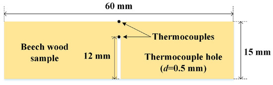
Figure 1.
Beech wood sample and the locations of thermocouples in constant HF ignition tests.

Table 1.
Key parameters of beech wood and optimized k and Cp.
2.2. Wood Ignition Tests under Power-Law Heat Fluxes
The experimental apparatus and procedures of wood ignition tests under power-law HFs are similar to those under constant HFs. The difference is that a proportion–integration–differentiation (PID) temperature controller, Delta DT320, was used to adjust the output power of the heater to achieve the power-law radiation. Meanwhile, an additional 0.5 mm diameter type K thermocouple was embedded inside the interior of sample to record the 6 mm in-depth temperature. In other words, surface, 3 and 6 mm in-depth temperatures were simultaneously collected in each test. Detailed information of sample dimensions and the locations of thermocouples are demonstrated in Figure 2. Originally, the impact of moisture content (based on dry weight) on ignition behaviors was examined using four moisture contents, 0%, 15%, 25% and 38%. However, only the measured temperatures of oven-dried samples were used for optimization to ensure consistency with other studies in the literature. Meanwhile, dry wood minimizes the effect of cracks during heating, which is intensified for moist wood. The calibrated power-law HFs can be expressed as:
where (kW m−2) is the transient HF, T is time, and a and b are positive rational numbers characterizing the increasing rate of HF. The values of a and b of the utilized four HFs are listed in Table 2.

Figure 2.
Beech wood sample and the locations of thermocouples in power-law HF ignition tests.
Table 2.
Values of a and b in the four calibrated power-law heat fluxes in wood ignition tests.
2.3. PMMA Ignition Tests under Linear Heat Fluxes
The PMMA ignition experiments were similar to those of wood under time-dependent HFs, and the difference was that finite thick samples, 1, 1.5, 3, 6 and 10 mm thick, and six linear HFs were used. Considering the fact that 1–6 mm thick PMMA samples suffered deformation during heating, especially for 1–3 mm ones, which significantly undermines the 1D premise of the numerical model, only the surface and in-depth temperatures of 10 mm thick samples were used for optimization. Detailed information of sample dimensions and the locations of thermocouples are demonstrated in Figure 3. The calibrated linear HFs can be expressed as:
where is an arbitrary initial HF, taken as 6.5 kW/m2 in our tests, and a is a constant determining the increasing rate of HF. The values of a of the six linear HFs are listed in Table 3. The relevant parameters of PMMA used in the numerical model and the optimized k and Cp, which are given in the following sections, are listed in Table 4.
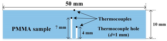
Figure 3.
PMMA sample and the locations of thermocouples in linear HF ignition tests.
Table 3.
Values of a in the six calibrated linear HFs in PMMA ignition tests.
Table 4.
Key parameters of PMMA and optimized k and Cp.
3. Numerical Model and PSO Algorithm
3.1. Numerical Model
A previously established 1D numerical model [28] involving solid pyrolysis and heat transfer in a multilayer composite was employed to simulate the measured surface and in-depth temperatures. Utilization of a 1D numerical model was determined by the experimental condition simulated. In all ignition tests, the four sides and bottom surface of samples were wrapped with thermal insulation material to minimize the heat loss on these surfaces, leaving only the top surface exposed to radiation. Such sample assembly follows the protocols in standard ignition/flammability tests, such as the cone calorimeter [26] and fire propagation apparatus (FPA) [32], to achieve a 1D heating condition. Consequently, using a 1D numerical model is appropriate. In the original model, a multilayer structure composed of different combustibles can be considered. However, in this study, only a thick layer, at least 10 mm thickness, was involved. Consequently, only the governing equation in this layer was introduced. Only surface absorption of radiation was considered, and in-depth absorption was ignored even for PMMA. Meanwhile, it was hypothesized that the evolved volatiles by pyrolysis are released instantaneously upon generation, and therefore no mass transfer is involved. Only the condensed phase is simulated, and the external heat flux from the heater is treated as the boundary condition. The energy and mass conservation equations are expressed as:
where ρ is the density, T is the temperature of solid, x is the spatial variable, r is the reflectivity of the solid surface, Sv is the pyrolysis rate, ΔHv is the reaction heat, T∞ is the environmental temperature, Cg is the specific heat of gas and is the mass flux in the controlled volume. The pyrolysis reaction rate can be written as:
where A is the pre-exponential factor, Ea is the activation energy and R is the ideal gas constant. The transient mass flux in a controlled volume at fixed location x and the total transient mass flux can be calculated as:
where l is the thickness of sample. The initial and boundary conditions are:
where ε, σ and hc are the absorptivity/emissivity of the top surface, Stefan–Boltzmann constant and convection coefficient of the top surface, respectively. The grid size and time step used were 0.05 mm and 0.5 s, respectively, and the duration time of simulation was determined by the relevant experimental results. More detailed information of the numerical model as well as the computation methodologies can be found in Ref. [28]. Since k and Cp are the target parameters in the following optimization process and pyrolysis of the solid exerts limited effect on surface and in-depth temperatures prior to ignition, thermal decomposition in the condensed phase is neglected to accelerate the convergency efficiency in optimization.
3.2. PSO Algorithm
The particle swarm optimization (PSO) algorithm was first proposed based on the process of finding the best feeding area for a flock of birds [33]. As an intelligent algorithm, PSO simulates the process of optimal decision making. It is assumed that at the beginning of foraging, the movement of the flock is chaotic, and over time the birds in random positions learn from each other and share foraging information within the flock. Each bird combines its own experience and the information transmitted by its peers to estimate the value of the current position to find food. Compared with other optimization algorithms, the PSO algorithm has higher convergence efficiency and accuracy [11]. In many optimization problems, the PSO algorithm converges to the optimal solution faster than GA. However, it also may fall into the local optimal solution, resulting in low convergence accuracy. Considering this drawback of PSO, the search range selection is carried out manually in current study to improve its convergence efficiency. PSO is applied to estimate temperature-dependent k and Cp of wood and PMMA combining the numerical model and experimentally measured temperatures at constant and time-dependent HFs.
In PSO, the input parameters of the numerical model excluding k and Cp were obtained from the literature, our previous publications, and experimental measurements. Then, several sets of temperature-dependent k and Cp of wood and PMMA were collected from the literature, and their average values of k and Cp were calculated. For each parameter, the lower bound of the search range was set to 0.1 times the average value, while the upper bound was determined to ensure the average value is also the mean value of the search range. Four constants need to be estimated in k and Cp expressions:
where k0, kT, Cp,0 and Cp,T are constants. The objective function necessary to quantify the discrepancy between experimental and numerical results in each iteration is defined as:
where Fobj is the objective function; the subscript h, exp and num denote the depth of the monitor point in tests (0, 3 and 6 mm), experimental and numerical results, respectively; and nexp is the total number of the experiment data points. The lower value of Fobj indicates better fitness and vice versa. The particle swarm size and the iteration number were selected to be 80 and 50, respectively. Combining the numerical model, heuristic optimization algorithms and experimental measurements to determine unknown properties is a common routine. More specifically, it is commonly called the curve-fitting method [34]. In this method, the experimental curves are simulated by the numerical model, and the target unknown parameters serving as inputs are adjusted by the PSO algorithm in each iteration until a prescribed error tolerance between numerical and experimental curves is achieved, indicating convergence. All computation was implemented using in-house MATLAB (2018b) code.
4. Results and Discussion
4.1. Optimization Results of Wood
In order to obtain more reliable k and Cp of wood, PSO is implemented at each constant HF, from 25 to 50 kW m−2, using experimentally measured surface and 3 mm in-depth temperatures, and the optimization results are compared with experimental data in Figure 4. In each experiment, at least three repeatable tests were conducted to guarantee the reproducibility and to estimate the experimental uncertainty. All the calculated uncertainty ranges reflected by the lengths of error bars can be found in Refs. [29,30,31]. Nevertheless, these error bars are not depicted in Figure 4 and the following figures to avoid potential location congestion. In all circumstances, the numerical profiles fit the experimental ones well despite some minor divergence since enforcing minimal discrepancy is essential for any optimization algorithm. In all subgraphs, the deviation of surface temperature is larger compared to 3 mm in-depth temperature, which is presumably due to the small cracks emerging over surface during heating and the generated thin char layer before ignition. These influential factors are not involved in the numerical model. Good fitness of 3 mm in-depth temperature is found in all subgraphs, which is particularly important for accurate prediction of k and Cp since these two parameters are highly relevant to the heat transfer inside the condensed phase.

Figure 4.
Comparison of wood surface and 3 mm in-depth temperatures between optimization and experimental results under different constant heat fluxes. Figure (a) shows a comparison of the optimized and experimental results for the wood surface and 3 mm in-depth temperatures under 25 kW/m2 constant heat flux. Figure (b) shows a comparison of the optimized and experimental results for the wood surface and 3 mm in-depth temperatures under 30 kW/m2 constant heat flux. Figure (c) shows a comparison of the optimized and experimental results for the wood surface and 3 mm in-depth temperatures under 40 kW/m2 constant heat flux. Figure (d) shows a comparison of the optimized and experimental results for the wood surface and 3 mm in-depth temperatures under 50 kW/m2 constant heat flux.
The optimized k and Cp of wood under each HF in Figure 4 are portrayed in Figure 5. Apparently, for each parameter, the optimized results at different HFs are very close to each, suggesting high accuracy of the optimization strategy. The average values of k and Cp are given in Figure 5a,b, respectively, and their linear temperature dependencies are listed in Table 1. Utilization of average values of k and Cp minimizes the potential impact of experimental system errors of each individual heat flux and improves the credibility of the final determined thermodynamics.
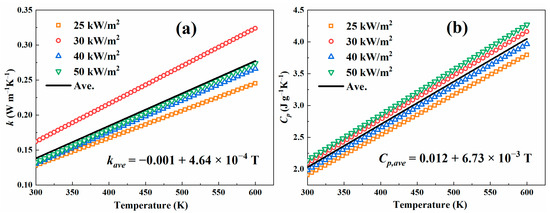
Figure 5.
Optimized temperature-dependent k and Cp of wood under constant heat fluxes and their average values. Where figure (a) shows the results for k and figure (b) shows the results for Cp.
A similar optimization strategy was also implemented for wood under the four power-law HFs listed in Table 2, and the comparison between experimental and numerical results are demonstrated in Figure 6. The difference is that an additional set of 6 mm in-depth temperatures were involved. Again, PSO was performed at each HF, and therefore four temperature-dependent expressions were obtained for k and Cp. Under all power-law HFs, the numerical curves fit the experimental ones well except for the end segments of surface temperature before ignition. Under power-law HFs, the heating times are much longer than those under constant HFs in Figure 5. As a result, the prolonged heating time facilitates the accumulation of yielded char layer over surface due to wood pyrolysis. Both wood pyrolysis and char oxidation were not considered in the numerical model, and therefore the measured surface temperatures were underpredicted. However, in the majority portion of surface temperature curve where the impact of pyrolysis can be ignored, the numerical model matches the experimental measurements well.
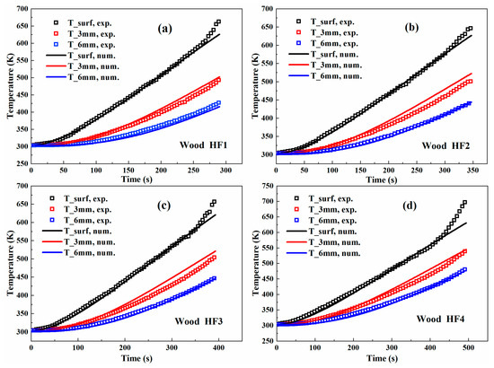
Figure 6.
Comparison of wood surface, 3 and 6 mm in-depth temperatures between optimization and experimental results under different power-law heat fluxes. Figure (a) shows a comparison of the optimization and experimental results for the wood surface, 3 and 6 mm in-depth temperatures under power-law heat flux in the form of HF1. Figure (b) shows a comparison of the optimization and experimental results for the wood surface, 3 and 6 mm in-depth temperatures under power-law heat flux in the form of HF2. Figure (c) shows a comparison of the optimization and experimental results for the wood surface, 3 and 6 mm in-depth temperatures under power-law heat flux in the form of HF3. Figure (d) shows a comparison of the optimization and experimental results for the wood surface, 3 and 6 mm in-depth temperatures under power-law heat flux in the form of HF4.
Again, the optimized k and Cp under the four power-law HFs and their average values are illustrated in Figure 7. A similar variation trend and moderate scatter are observed in each group. The attained average k and Cp are listed in Table 1.

Figure 7.
Optimized temperature-dependent k and Cp of wood under power-law heat fluxes and their average values. Where figure (a) shows the results for k and figure (b) shows the results for Cp.
The optimized average k and Cp of beech wood at constant and power-law HFs were compared with the reported ones in Refs. [29,35], as demonstrated in Figure 8. In Gong’s [29] work, these two parameters were optimized using GA under different constant HFs, while in Ross’s [35] study they were directly measured by experimental methods, and therefore constant k was obtained, and the linear temperature dependency of Cp was only applicable in a narrow temperature range. In Figure 8a, both the optimized k under constant and power-law HFs in current study agree relatively well with the one in Ref. [29] but are slightly higher than the constant value in Ref. [35]. In Figure 8b, our optimized Cp at constant HF agrees well with the one in Gong’s [29] work where the same experimental data but also the GA algorithm were utilized. This agreement again confirms the high reliability of the optimization strategy employed in this study. Meanwhile, the optimized Cp of wood at power-law HF fits Ross’s [35] result well. The relatively large divergence between the two sets of Cp is primarily attributed to the contained moisture content in wood samples of constant HF tests [29]. In normal environment conditions, the moisture content of wood typically varies in the range of 8–10% [35]. However, in power-law HF tests [30] and Ref. [35], the wood samples were oven-dried. A high value of Cp of water caused this discrepancy.

Figure 8.
Comparison of k and Cp of beech wood between optimized results with the reported values in the literature [29,35]. Where figure (a) shows the results for k and figure (b) shows the results for Cp.
4.2. Optimization Results of PMMA
Similar optimization procedures were also conducted for PMMA under the six linear HFs in Table 3, and the comparison between experimental and numerical results is depicted in Figure 9. Under all linear HFs, good agreement is observed despite some minor divergence. The small disagreements of in-depth temperatures in Figure 9a–c are presumably caused by the potential inaccurate locations of the thermocouple beads during tests, while the slight overprediction of surface temperature at the end segments is associated with the neglect of endothermic pyrolysis reaction of PMMA. Furthermore, the average values of k and Cp, listed in Table 4, based on the six optimization runs were plotted and compared with the reported ones in Stoliarov’s [36] work, as shown in Figure 10. Both our optimized k and Cp show similar variation trends to those in Ref. [36] though piecewise functions are used in that work. The discrepancy between our and Stoliarov’s results may be attributed to the different types and processing of PMMA used.
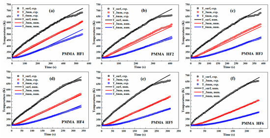
Figure 9.
Comparison of PMMA surface, 3 and 6 mm in-depth temperatures between optimization and experimental results under different linear heat fluxes. Figure (a) shows a comparison of the optimization and experimental results for the PMMA surface, 3 and 6 mm in-depth temperatures under linear heat flux in the form of HF1. Figure (b) shows a comparison of the optimization and experimental results for the PMMA surface, 3 and 6 mm in-depth temperatures under linear heat flux in the form of HF2. Figure (c) shows a comparison of the optimization and experimental results for the PMMA surface, 3 and 6 mm in-depth temperatures under linear heat flux in the form of HF3. Figure (d) shows a comparison of the optimization and experimental results for the PMMA surface, 3 and 6 mm in-depth temperatures under linear heat flux in the form of HF4. Figure (e) shows a comparison of the optimization and experimental results for the PMMA surface, 3 and 6 mm in-depth temperatures under linear heat flux in the form of HF5. Figure (f) shows a comparison of the optimization and experimental results for the PMMA surface, 3 and 6 mm in-depth temperatures under linear heat flux in the form of HF6.

Figure 10.
Comparison of k and Cp of PMMA between optimized results and the reported ones in Ref. [36]. Where figure (a) shows the results for k and figure (b) shows the results for Cp.
4.3. Parameter Validation
The reliability of the optimized k and Cp was verified by simulating the experimental temperatures that were not utilized in parameterization. Figure 11 shows experimental surface, 3 and 6 mm in-depth temperatures of wood under a power-law HF, HF1 in Table 2, and the corresponding simulation results using the optimized k and Cp at constant HF in Table 1. Apparently, the numerical model successfully captures the measured surface temperature except for the end segment. Nevertheless, moderate and unacceptable discrepancies are observed for 3 and 6 mm in-depth temperatures. These deviations are mainly attributable to the existence of moisture content in wood samples in constant HF tests as discussed in the preceding section. Higher k and Cp at constant HF lead to lower predicted in-depth temperatures as depicted in Figure 11. However, the moisture content at the surface is eliminated quickly after exposure of radiation and thus has little impact on surface temperature history.

Figure 11.
Validation of optimized k and Cp of wood under constant HFs by comparing experimental and numerical results of power-law heat flux of HF1.
Reliability of the optimized k and Cp of wood under constant HF of 25 kW m−2 can also be verified by predicting the experimental temperatures of other three constant HFs, 30, 40 and 50 kW m−2, as shown in Figure 12. Obviously, under all the examined HFs, the numerical curves fit the experimental data well. Similarly, the optimized k and Cp of wood under each HF of 30, 40 and 50 kW m−2 can be validated using the same method. Meanwhile, the optimized k and Cp of wood under each power-law HF can also be verified by simulating the experimental measurements of the remaining power-law HFs. Good agreement is detected in all these validation cases, and they are not exhibited for concision.

Figure 12.
Validation of optimized k and Cp of wood under 25 kW m−2 constant heat flux of by comparing experimental and numerical results of constant heat fluxes of 30, 40 and 50 kW m−2. Figure (a) compares the experimental and numerical results of constant heat flux of 30 kW m−2. Figure (b) compares the experimental and numerical results of constant heat flux of 40 kW m−2. Figure (c) compares the experimental and numerical results of constant heat flux of 50 kW m−2.
A similar validation methodology was further implemented for PMMA under linear HF, as demonstrated in Figure 13 where the optimized k and Cp under linear HF of HF 4 are verified under the other five linear HFs. In all validation cases, the numerical model well captures the variation trends and magnitudes of all surface, 3 and 6 mm in-depth temperatures, which again implies high credibility and accuracy of the optimization method and numerical model.

Figure 13.
Validation of optimized k and Cp of PMMA under linear heat flux of HF4 by comparing experimental and numerical results of the remaining linear HFs. The experimental and numerical results under linear heat flux of HF1 are represented in Figure (a). The experimental and numerical results under linear heat flux of HF2 are represented in Figure (b). The experimental and numerical results under linear heat flux of HF3 are represented in Figure (c). The experimental and numerical results under linear heat flux of HF5 are represented in Figure (d). The experimental and numerical results under linear heat flux of HF6 are represented in Figure (e).
4.4. Impact of Search Range on PSO
In the tests described in the preceding sections, the lower bound of the search range during PSO was set to 0.1 times the manually selected average value, while the upper bound was determined to ensure the selected average value was also the mean value of the search range. In order to examine the impact of search range on optimization results, an additional expanded large search range was employed to implement the optimization. The lower bound of the large search range is 0.01 times the selected average value, while the upper bound was obtained through the same strategy as mentioned above. Wood experimental results under 25 kW m−2 constant HF were used to conduct the optimization, and the comparison is illustrated in Figure 14, where LSR and SSR denote large and small search ranges, respectively. When using SSR, good agreement is found for both surface and 3 mm in-depth temperatures, implying convergence and high accuracy. However, if LSR is used, appreciable divergence emerges even though the objective function, Fobj in Equation (11), remains unchanged with increasing iterations during optimization, suggesting convergence. This unacceptable deviation is presumably caused by the inherent flaw of the PSO algorithm in that it may be trapped in a local optimal solution [12]. Therefore, it can be concluded that utilization of a reasonable narrow search range can effectively suppress the potential occurrence of local optimal solution. Meanwhile, a reasonable narrow search range can also effectively diminish the potential compensation effect, which is still an unsolved issue in determining unknown parameters using the optimization algorithm as interpreted by Vyazovkin [37].
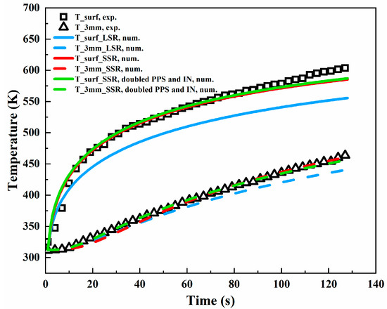
Figure 14.
Effects of search range, particle swarm size (PSS) and iteration number (IN) on PSO results in the case where wood experimental temperatures under 25 kW m−2 constant heat flux are used.
Particle swarm size (PSS) and iteration number (IN) in PSO may also pose a nonnegligible impact on optimization results. To investigate their effects, an additional optimization run where both PSS and IN were doubled was implemented using the same experimental data and the same SSR, and the optimization results are depicted in Figure 14. Apparently, little discrepancy exists between the original case and the modified case, implying the original PSS and IN are sufficiently high for accurate optimization and convergence.
5. Conclusions
Two important thermodynamic parameters, k and Cp, of two representative solid combustibles, beech wood and PMMA, were quantitatively determined by the PSO algorithm, a 1D numerical model and the related measured surface and in-depth temperatures in ignition tests under constant, power-law and linear HFs. Linearized temperature-dependent k and Cp were obtained through the employed approach. In each set of HFs, the optimization was carried out under each HF, and the average value was deemed the final result. For wood at constant HFs, good agreement was found between experimental and optimization results, and the scatter among the optimized thermodynamics is relatively small, implying high accuracy of the utilized method, while under power-law HFs, good fitness was also observed for surface and in-depth temperatures of wood. Larger scatter of the optimized thermodynamics was detected, and an alternative pair of k and Cp was obtained. All these thermodynamic parameters fell into the same ranges of the reported ones in the literature. The deviation of these two sets of k and Cp was attributed to the moisture content difference of the utilized samples. Subsequently, the same optimization strategy was further implemented for PMMA under six linear HFs. Good agreement was again found for surface and in-depth temperatures under all HFs, and the attained k and Cp matched the correlations reported in the literature well. Credibility of the optimized wood thermodynamics under constant HFs was verified by emulating the measured temperatures of wood under a power-law HF, and good agreement existed for surface temperature. The divergences for 3 and 6 mm in-depth temperatures were caused by moisture content difference. Additionally, the optimized thermodynamics of wood at 25 kW m−2 were validated by predicting the experimental temperatures under the remaining constant HFs. Meanwhile, the optimized thermodynamics of PMMA under HF4 were verified by simulating the measured temperatures under the remaining linear HFs. In all these scenarios, the numerical curves matched the experimental data well, suggesting high reliability of the obtained k and Cp. Furthermore, the impact of search range of PSO on optimization results was investigated by using an additional expanded search range. The outcomes showed that larger search range featured a higher possibility of being trapped in local optimal solution, and therefore a narrow search range is strongly suggested. Using doubled particle swarm size and iteration number had little effect on optimization results, indicating the originally adopted values were sufficiently high for convergence.
A potential weakness of current study is the fact that pyrolysis in the solid before ignition was ignored. This assumption is reasonable and would introduce negligible influence for piloted ignition wherein pyrolysis exerts little impact [34]. Nevertheless, this hypothesis is unacceptable for autoignition, where intense thermal decomposition occurs in the vicinity of surface before ignition, implying pyrolysis cannot be neglected. Accurate predictions of surface temperature and mass loss rate necessitate full knowledge of pyrolysis kinetics. In other words, kinetic parameters, such as preexponential factor and activation energy in the Arrhenius equation can also be quantitatively estimated by inversely modeling the measured temperatures and mass loss rate during autoignition or combustion using proper optimization algorithms. All these deserve further in-depth exploration in future work.
Author Contributions
Conceptualization, J.G.; Methodology, H.P.; Validation, H.P.; Formal analysis, J.G.; Investigation, H.P. and J.G.; Resources, J.G.; Data curation, H.P.; Writing—original draft, H.P.; Writing—review & editing, J.G.; Visualization, H.P.; Supervision, J.G.; Project administration, J.G.; Funding acquisition, J.G. All authors have read and agreed to the published version of the manuscript.
Funding
This research was funded by National Natural Science Foundation of China (51974164), Natural Science Foundation of Jiangsu Province of China (BK20221311) and University Natural Science Research Project in Jiangsu Province (21KJA620002).
Acknowledgments
The authors gratefully appreciate this support.
Conflicts of Interest
The authors declare no conflict of interest.
References
- Cueff, G.; Mindeguia, J.; Dréan, V.; Breysse, D.; Auguin, G. Experimental and numerical study of the thermomechanical behaviour of wood-based panels exposed to fire. Constr. Build. Mater. 2018, 160, 668–678. [Google Scholar] [CrossRef]
- Ferreiro, A.I.; Rabaçal, M.; Costa, M. A combined genetic algorithm and least squares fitting procedure for the estimation of the kinetic parameters of the pyrolysis of agricultural residues. Energy Convers. Manag. 2016, 125, 290–300. [Google Scholar] [CrossRef]
- Lokmane, A.; Sébastien, L.; Lamiae, V.; Laurent, B.; Bechara, T. Comparative investigation for the determination of kinetic parameters for biomass pyrolysis by thermogravimetric analysis. J. Therm. Anal. Calorim. 2017, 129, 1201–1213. [Google Scholar]
- Ding, Y.M.; Zhang, Y.; Zhang, J.Q.; Zhou, R.; Ren, Z.Y.; Guo, H.L. Kinetic parameters estimation of pinus sylvestris pyrolysis by Kissinger-Kai method coupled with Particle Swarm Optimization and global sensitivity analysis. Bioresour. Technol. 2019, 293, 122079. [Google Scholar] [CrossRef] [PubMed]
- Ding, Y.M.; Huang, B.Q.; Li, K.Y.; Du, W.Z.; Lu, K.H.; Zhang, Y.S. Thermal interaction analysis of isolated hemicellulose and cellulose by kinetic parameters during biomass pyrolysis. Energy 2020, 195, 117010. [Google Scholar] [CrossRef]
- Ding, Y.M.; Zhang, J.; He, Q.Z.; Huang, B.Q.; Mao, S.H. The application and validity of various reaction kinetic models on woody biomass pyrolysis. Energy 2019, 179, 784–791. [Google Scholar] [CrossRef]
- Ding, Y.M.; Wang, C.J.; Chaos, M.; Chen, R.Y.; Lu, S.X. Estimation of beech pyrolysis kinetic parameters by Shuffled Complex Evolution. Bioresour. Technol. 2016, 200, 658–665. [Google Scholar] [CrossRef]
- Fiola, G.J.; Chaudhari, D.M.; Stoliarov, S.I. Comparison of pyrolysis properties of extruded and cast Poly (methyl methacrylate). Fire Saf. J. 2021, 120, 103083. [Google Scholar] [CrossRef]
- Richter, F.; Rein, G. Pyrolysis kinetics and multi-objective inverse modelling of cellulose at the microscale. Fire Saf. J. 2017, 91, 191–199. [Google Scholar] [CrossRef]
- Gong, J.H.; Gu, Y.M.; Zhai, C.J.; Wang, Z.R. A hybrid pyrolysis mechanism of phenol formaldehyde and kinetics evaluation using isoconversional methods and genetic algorithm—ScienceDirect. Thermochim. Acta. 2020, 690, 178708. [Google Scholar] [CrossRef]
- Ding, Y.M.; Zhang, W.L.; Yu, L.; Lu, K.H. The accuracy and efficiency of GA and PSO optimization schemes on estimating reaction kinetic parameters of biomass pyrolysis. Energy 2019, 176, 582–588. [Google Scholar] [CrossRef]
- Sun, J.; Wu, X.; Palade, V.; Fang, W.; Lai, C.; Xu, W. Convergence analysis and improvements of quantum-behaved particle swarm optimization. Inform. Sci. 2012, 193, 81–103. [Google Scholar] [CrossRef]
- Nimmanterdwong, P.; Chalermsinsuwan, B.; Piumsomboon, P. Optimizing utilization pathways for biomass to chemicals and energy by integrating emergy analysis and particle swarm optimization (PSO). Renew. Energy 2023, 202, 1448–1459. [Google Scholar] [CrossRef]
- Xu, L.; Jiang, Y.; Wang, L. Thermal decomposition of rape straw: Pyrolysis modeling and kinetic study via particle swarm optimization. Energy Convers. Manag. 2017, 146, 124–133. [Google Scholar] [CrossRef]
- Shorabeh, S.N.; Samany, N.N.; Minaei, F.; Firozjaei, H.K.; Homaee, M.; Boloorani, A.D. A decision model based on decision tree and particle swarm optimization algorithms to identify optimal locations for solar power plants construction in Iran. Renew. Energy 2022, 187, 56–67. [Google Scholar] [CrossRef]
- Srinivasan, B.; Mekala, P. Mining social networking data for classification using Reptree. Int. J. Adv. Res. Comput. Sci. Manag. Stud. 2014, 2, 155–160. [Google Scholar]
- Aghbashlo, M.; Tabatabaei, M.; Nadian, M.H.; Davoodnia, V.; Soltanian, S. Prognostication of lignocellulosic biomass pyrolysis behavior using ANFIS model tuned by PSO algorithm. Fuel 2019, 253, 189–198. [Google Scholar] [CrossRef]
- Zhao, S.H.; Xu, W.J.; Chen, L.H. The modeling and products prediction for biomass oxidative pyrolysis based on PSO-ANN method: An artificial intelligence algorithm approach. Fuel 2022, 312, 122966. [Google Scholar] [CrossRef]
- Sunphorka, S.; Chalermsinsuwan, B.; Piumsomboon, P. Artificial neural network model for the prediction of kinetic parameters of biomass pyrolysis from its constituents. Fuel 2017, 193, 142–158. [Google Scholar] [CrossRef]
- Abiodun, O.I.; Jantan, A.; Omolara, A.E.; Dada, K.V.; Mohamed, N.A.; Arshad, H. State-of-the-art in artificial neural network applications: A survey. Heliyon 2018, 4, 11. [Google Scholar] [CrossRef]
- Ghose, A.; Gupta, D.; Nuzelu, V.; Rangan, L.; Mitra, S. Optimization of laccase enzyme extraction from spent mushroom waste of Pleurotus florida through ANN-PSO modeling: An ecofriendly and economical approach. Environ. Res. 2023, 222, 115345. [Google Scholar] [CrossRef] [PubMed]
- Zhu, S.P.; Keshtegar, B.; Seghier, M.B.; Zio, E.; Taylan, O. Hybrid and enhanced PSO: Novel first order reliability method-based hybrid intelligent approaches. Comput. Methods Appl. Mech. Eng. 2022, 393, 114730. [Google Scholar] [CrossRef]
- Lin, S.W.; Liu, A.; Wang, J.G.; Kong, X.Y. An intelligence-based hybrid PSO-SA for mobile robot path planning in warehouse. J. Comput. Sci. 2023, 67, 101938. [Google Scholar] [CrossRef]
- Kardani, N.; Bardhan, A.; Samui, P.; Nazem, M.; Asteris, P.G.; Zhou, A.N. Predicting the thermal conductivity of soils using integrated approach of ANN and PSO with adaptive and time-varying acceleration coefficients. Int. J. Therm. Sci. 2022, 173, 107427. [Google Scholar] [CrossRef]
- Du, W.Y.; Ma, J.; Yin, W.J. Orderly charging strategy of electric vehicle based on improved PSO algorithm. Energy 2023, 271, 127088. [Google Scholar] [CrossRef]
- ASTM E1354; Standard TEST method for Heat and Visible Smoke Release Rates for Materials and Products Using an Oxygen Consumption Calorimeter. ASTM International: West Conshohocken, PA, USA, 2011.
- Swann, J.D.; Ding, Y.; McKinnon, M.B.; Stoliarov, S.I. Controlled atmosphere pyrolysis apparatus II (CAPA II): A new tool for analysis of pyrolysis of charring and intumescent polymers. Fire Saf. J. 2017, 91, 130–139. [Google Scholar] [CrossRef]
- Gong, J.H.; Zhu, Z.X.; Zhai, C.J. A numerical model for simulating pyrolysis and combustion behaviors of multilayer composites. Fuel 2021, 289, 119752. [Google Scholar] [CrossRef]
- Gong, J.H.; Zhai, C.J.; Wang, Z.R. Pyrolysis and autoignition behaviors of beech wood coated with an acrylic-based waterborne layer. Fuel 2021, 306, 121724. [Google Scholar] [CrossRef]
- Gong, J.H.; Cao, J.L.; Zhai, C.J.; Wang, Z.R. Effect of moisture content on thermal decomposition and autoignition of wood under power-law thermal radiation. Appl. Therm. Eng. 2020, 179, 115651. [Google Scholar] [CrossRef]
- Gong, J.H.; Zhang, M.R.; Zhai, C.J.; Yang, L.Z.; Zhou, Y.; Wang, Z.R. Experimental, analytical and numerical investigation on auto-ignition of thermally intermediate PMMA imposed to linear time-increasing heat flux. Appl. Therm. Eng. 2020, 172, 115137. [Google Scholar] [CrossRef]
- ASTM E2058-13a; Standard test Methods for Measurement of Synthetic Polymer Material Flammability Using a Fire Propagation Apparatus (FPA). ASTM International: West Conshohocken, PA, USA, 2013.
- Eberhart, R.C.; Kennedy, J. A new optimizer using particle swarm theory. In Proceedings of the sixth international symposium on micro machine and human science 1995, Nagoya, Japan, 4–6 October 1995. [Google Scholar]
- Gong, J.; Yang, L. A Review on Flaming Ignition of Solid Combustibles: Pyrolysis Kinetics, Experimental Methods and Modelling. Fire Technol. 2022, 1–98. [Google Scholar] [CrossRef]
- Ross, R.J. Wood Handbook: Wood as an Engineering Material; Forest Products Laboratory, United States Department of Agriculture Forest Service: Washington, DC, USA, 1987. [Google Scholar]
- Stoliarov, S.I.; Crowley, S.; Lyon, R.E. Prediction of the burning rates of non-charring polymers. Combust. Flame 2009, 156, 1068–1083. [Google Scholar] [CrossRef]
- Vyazovkin, S.; Burnham, A.K.; Favergeon, L.; Koga, N.; Moukhina, E.; Perez-Maqueda, L.A.; Sbirrazzuolie, N. ICTAC Kinetics Committee recommendations for analysis of multi-step kinetics. Thermochim Acta. 2020, 689, 178597. [Google Scholar] [CrossRef]
Disclaimer/Publisher’s Note: The statements, opinions and data contained in all publications are solely those of the individual author(s) and contributor(s) and not of MDPI and/or the editor(s). MDPI and/or the editor(s) disclaim responsibility for any injury to people or property resulting from any ideas, methods, instructions or products referred to in the content. |
© 2023 by the authors. Licensee MDPI, Basel, Switzerland. This article is an open access article distributed under the terms and conditions of the Creative Commons Attribution (CC BY) license (https://creativecommons.org/licenses/by/4.0/).