Abstract
The parameter identification of a PEMFC is the process of using optimization algorithms to determine the ideal unknown variables suitable for the development of an accurate fuel-cell-performance prediction model. These parameters are not always available from the manufacturer’s datasheet, so they need to be determined to accurately model and predict the fuel cell’s performance. Five optimization methods—bald eagle search (BES) algorithm, equilibrium optimizer (EO), coot (COOT) algorithm, antlion optimizer (ALO), and heap-based optimizer (HBO)—are used to compute seven unknown parameters of a PEMFC. During optimization, these seven parameters are used as decision variables, and the fitness function to be minimized is the sum square error (SSE) between the estimated cell voltage and the actual measured cell voltage. The SSE obtained for the BES algorithm was noted to be 0.035102. The COOT algorithm recorded an SSE of 0.04155, followed by ALO with an SSE of 0.04022 and HBO with an SSE of 0.056021. BES predicted the performance of the fuel cell accurately; hence, it is suitable for the development of a digital twin for fuel-cell applications and control systems for the automotive industry. Furthermore, it was deduced that the convergence speed for BES was faster compared to the other algorithms investigated. This study aims to use metaheuristic algorithms to predict fuel-cell performance for the development and commercialization of digital twins in the automotive industry.
1. Introduction
For both small power uses and bigger industrial applications, clean energy sources are becoming increasingly necessary due to the rapid decline in fossil fuel sources and the growing demand for electricity [1]. Harnessing energy from renewable sources such as solar and wind is often relied on, but these sources are affected by environmental conditions, which has led to the development of fuel cells to help supplement existing green energy sources. Fuel cells have traditionally been divided into stationary, portable, or transportation types [2]. Fuel-cell technology has advanced quickly in the automotive sector due to the growing usage of fuel cells for heavy-duty land vehicles such as public buses. Stationary fuel cells for homes and businesses have also become more popular [3]. Stationary fuel cells have a variety of applications. Several businesses and researchers have developed a keen interest in fuel cells in recent years. The chemical energy produced by the reaction between oxygen and hydrogen, or natural air, can be quickly converted into electrical energy by fuel cells [4]. Many fuel-cell types exist, such as alkaline, solid oxide, proton exchange membrane, and phosphoric acid fuel cells [5]. Each of these types of fuel cells has its own use, but the most common type of fuel cell used in the automotive industry is the PEMFC [6,7]. The advantages of PEMFCs include their high efficiency, low emissions, high power density, and the ability to be quickly refueled. PEMFCs can be used to power many types of applications, including transportation, standby power, residential, and industrial applications. Additionally, PEMFC technology is relatively simple and cost-effective when compared to other fuel-cell technologies. The No Free Lunch Theorem states that any optimization algorithm will have no performance advantage over any other algorithm when averaged over all possible problems. This follows from the fact that any algorithm must make assumptions and trade-offs to optimize a problem. Any such assumptions can be beneficial for some problems while detrimental for others. The accuracy of the mathematical model for a PEMFC is highly dependent on the amount of manufacturer information available. Therefore, the unknown parameters for PEMFCs must be clearly defined to establish a perfect agreement between the experimental and mathematical models. The chemical characteristic within the cell is a key determinant of the output voltage of the cell [8]. There are currently some concepts established in the literature capable of estimating the exact PEMFC parameters. Most of these optimization-based approaches are considered as being simple, consistent, and robust [9]. In terms of the optimal parameters in relation to PEMFCs, several investigations have been carried out in the literature. For instance, a multiverse optimizer was explored for the determination of the parameters for a PEMFC-equivalent circuit [10]. The total number of parameters considered in the study was seven. Other authors equally reported various optimization parameters capable of ensuring convergence [11]. There was a clear classification of the various methods, specifically involving evolutionary-based, swarm physics as well as nature. Hegazy et al. [12] also evaluated various metaheuristics in the optimization of microgrids. To reduce the sum squared error (SSE), adaptive sparrow search algorithms were also explored to evaluate the variation between the calculated and measured voltage [13]. Yousri et al. [14] concluded that the fractional-order-modified Harris hawk optimizer was the best algorithm for the mathematical modeling of PEMFCs. To further reduce the disparity between the estimated and empirical results, other authors used a developed coyote optimization algorithm [15]. Yuan et al. [15] carried out the investigation using two types of fuel cells. The application of an improved monarch butterfly optimizer has also been explored in determining unknown parameters to ensure a reduction in the integral time absolute error [16]. With varying conditions around the cell, two types of cells were also studied (2 kW Nexa and 6 kW Nedstack PS6) using an improved chimp optimizer [17]. The improved chimp optimizer was also evaluated for three commercial fuel cells. A 15-nature algorithm was used to validate the outcome of the study. Tabbi et al. [18] concluded that the artificial ecosystem-based algorithm presented a better result compared to the grey wolf optimizer, particle swarm optimizer, slime mold algorithm, and Harris hawk optimizer [18]. A hybrid method comprising a combination between a vortex search algorithm and differential evolution for the identification of the optimal parameters for PEMFCs has also been presented in the literature [19]. The SSE was considered as the ideal fitness function between the experimental voltages and those generated for the stack deduced mathematically. A monarch butterfly optimizer was also experimented on a 250 W PEMFC stack under varying conditions [20]. A further investigation also evaluated the ideal parameters for PEMFCs by considering the SSE between experimental and numerical data using metaheuristics [21]. A slime mold optimizer was also used by Gupta et al. for the determination of the unknown parameters for PEMFCs [22]. An improved search optimizer for evaluating the parameters for PEMFCs was also investigated by Qin et al. [23]. The SSE between the experimental and estimated data was considered as the target. A Bayesian-regularized neural network was adopted in extracting the ideal parameters for PEMFCs [24]. Using a sunflower optimizer, an estimation of the unknown parameters for PEMFCs was carried out by Yuan et al. [25]. A converged moth search algorithm has also been reported in the literature to be suitable in reducing the SSE between the measured and experimental voltages [26]. BCS 500 stack and Nedstack PS6 data were used for the study. A bi-subgroup algorithm for extracting the unknown parameters from PEMFCs has also been reported in the literature [27]. Syah et al. [28] used a balanced strider method in reducing the total squared variation between experimental and numerical voltages. The cost of the stack was also utilized as the target using a modified grass fibrous root algorithm [29]. Using three types of fuel cells (BCS 500/250 and Nedstack PS6), a particle swarm optimizer was utilized in the identification of the best parameters for the fuel cell [30]. Mossa et al. [31] used two optimizers (Harris hawk and atom search algorithm) mainly for estimating the unknown values for PEMFCs. The SSE value recorded for the measured and mathematical data was taken as the fitness function. Rezk et al. [32] utilized a gradient-based algorithm for the determination of the ideal parameters between three types of fuel cells and compared it with other algorithms. A chaos owl search optimizer has also been adopted to reduce the sum squared deviation for measured as well as mathematically determined voltages [33]. A chaotic binary shark smell optimizer was also adopted for the estimation of the unknown data for a PEMFC [34]. A heterogeneous comprehensive learning Archimedes optimizer was also adopted for determining the unknown parameters for fuel cells [35]. A deer hunting algorithm has also been adopted in estimating the parameters for a PEMFC. The study also involved the application of artificial neural networks [36]. A water cycle algorithm was equally harnessed in estimating the unknown values for PEMFCs [37]. An enhanced bald eagle search algorithm has also been reported in the literature as being ideal for exploring the unknown values [38] using the SSE as the target for reducing the values between the measured and estimated data. A coyote optimizer was employed by Abaza et al. [39] for estimating the unknown parameters. The utilization of a semi-empirical model for PEMFCs has equally been reported using the SSE as the target [40]. By reducing the integral absolute error between the various types of voltages, Lu et al. [41] explored the application of a crow search approach in the determination of unknown parameters. An equilibrium optimizer has equally been adopted for estimating the unknown values for fuel cells [42]. A satin bowerbird algorithm has been captured in the literature as being suitable for the estimation of the ideal parameters for developing polarization curves [43]. An L-SHADE-EpSin approach was used in the literature in the development of a model for PEMFC estimation [44]. Isa et al. [45] equally explored the application of an antlion as well as a dragonfly optimizer for estimating the unknown parameters for PEMFCs. The identification of fuel PEMFC parameters has also been explored using Harris hawk algorithms by Song et al. [46]. A barnacles mating optimizer was also explored in modeling the fuel-cell behavior accurately [47]. An Archimedes optimizer was also used in the literature mainly for reducing the deviation between the data gathered from the experimental and mathematical models [48]. A transient search optimizer was also reported as being suitable in accurately estimating the unknown parameters for PEMFCs [49]. Calasan et al. [50] used the Lambert W function in reducing the deviation between measured as well as simulated voltages. This study, however, presents the accurate prediction of the seven unknown parameters of PEMFCs often not available in the manufacturer’s data sheet. The study further corroborates the prospects of metaheuristic algorithms in the development of a digital twin for PEMFCs, paying critical attention to the sum squared error, which is the objective function, and the computational time for the entire predictive process. Section 2 of the investigation captures the detailed information regarding the electrochemical reaction of a PEMFC, while Section 3 highlights the information on the PEMFC-parameter-estimation approach and Section 4 delves more into the bald eagle search (BES) algorithm. A summary of the experimental procedure is found in Section 5, and the results are summarized and discussed in Section 6. The main findings are outlined in Section 7 to reflect on the overall outcome of the study.
2. Electrochemical Reaction Inside a PEMFC
The electrochemical reaction inside a PEMFC involves the oxidation of fuel molecules at the anode and the reduction in oxygen molecules at the cathode. Protons (H+) are generated at the anode and flow across an electrolyte membrane to the cathode [51]. This electrochemical reaction produces water, heat, and electricity. Figure 1 presents the various compositions of a fuel cell. As can be observed, the various electrodes (anode and cathode) are separated by a membrane. The membrane is designed to be permeable to only protons. Furthermore, there is the presence of a catalyst to speed up the electrochemical reaction [52]. The cell is designed to ensure that when the hydrogen fuel reaches the membrane, it dissociates into two ions. Due to the morphological composition of the membrane, the protons go through the membrane to the cathodic electrode, while the electrons go through an external circuit to produce electricity and water as a byproduct of the reaction. The overall reaction within the cell is summarized in Equations (1)–(3) [51].
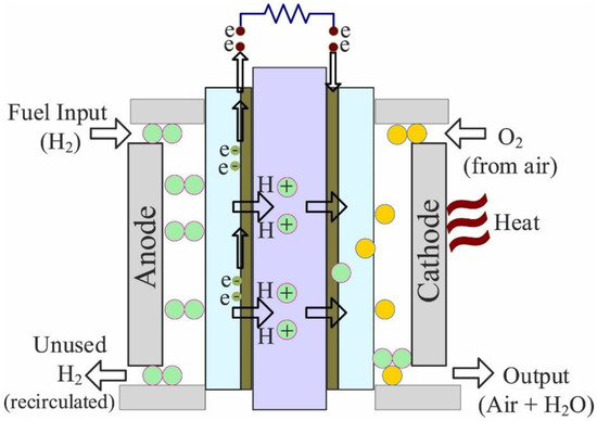
Figure 1.
Electrochemical reaction in a PEMFC [52].
Anode
Cathode
Complete chemical reaction
Fuel Cell Modeling Mathematically
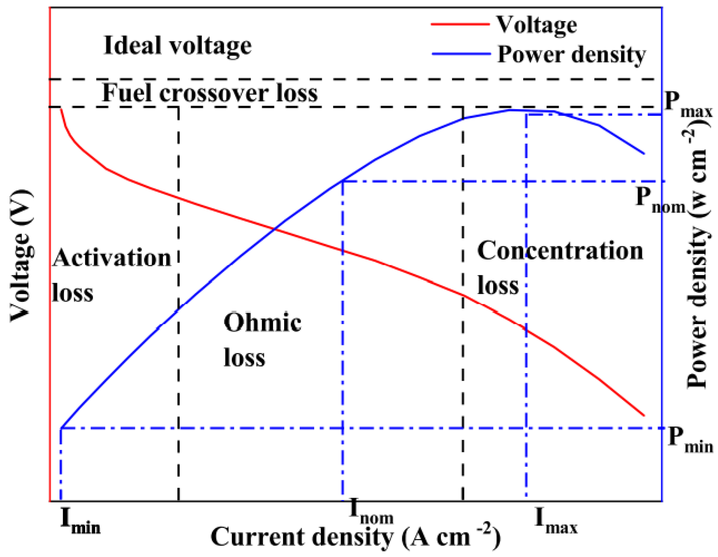
For both small power uses and bigger industrial applications, clean energy sources are becoming increasingly necessary due to the rapid decline in fossil fuel sources and the growing demand for electricity [50]. Harnessing energy from renewables is often relied on, but these sources are affected by environmental conditions, which has led to the development of fuel cells to help supplement existing green energy sources. Fuel cells have traditionally been divided into stationary, portable, or transportation types [51,52]. The polarization curve for a fuel cell being operated at 80 °C is captured in Figure 2. It can be noticed that there are three main areas on the polarization curve. These areas are broadly known as activation losses, ohmic losses, and concentration losses [53]. There is no linearity within the activation region. The activation region presents holistic information regarding the electrochemical reaction within the cell. The ohmic losses are commonly found within the membrane. The final section is the mass concentration losses due to variations in the concentration gradient within the cell [54]. The total cell voltage is depicted in Equation (4) as [53].

Figure 2.
Various types of losses in a fuel cell.
denotes the open circuit voltage, while represents the activation polarization; is the ohmic loss, and is the concentration loss [54]. It is also evident that within the ohmic section, the output voltage is dependent on the current density. The slope is also obtained based on the ionic resistance of the electrolyte, as explained earlier. The concentration loss is due to mass transfer limitations leading to a sharp decline in the voltage to zero. Increasing the total output voltage () of the cell is dependent on the number of cells () connected in a series, as depicted in Equation (5) [50].
is basically the open circuit voltage, which is determined using the Nernst equation [55], but other parameters that consider the variation in temperature surrounding the cell are also taken into account, as depicted in Equation (6) [50].
The temperature for the cell is represented as , while the partial pressure of oxygen is and that of hydrogen is . Equations (7) and (8) denote the various partial pressure parameters represented mathematically [51,52].
The anodic relative humidity is represented as , while that of the cathode is . The anode pressure at the inlet is , while that at the cathode is . The area of the cell is captured as A, while the current is . The water vapor saturation is , and this parameter has a direct correlation to temperature T, as captured in Equation (9). On the other hand, Equation (10) is utilized in the determination of the activation losses. are semi-empirical parametric coefficients, while oxygen concentration is highlighted as and computed using Equation (11). Calculating the ohmic losses is achieved using Equation (12) [52].
denote the electronic and ionic resistance, respectively. The electronic resistance is attributed to the slightest perturbations in relation to the current and voltage, and Equation (13) [50] is utilized to calculate this mathematically, while the membrane parametric coefficient is determined using Equation (14). Equation (15) [51] is utilized in computing the concentration polarization mathematically. b is the parametric coefficient, sometimes referred to as the diffusion parameter, and the maximum current density is Jmax, while J is the actual current density.
3. PEMFC-Parameter-Estimation Approach
In developing a computational model for PEMFCs mathematically, the calculation of the specific seven model parameters ( is very important. The major setback here is the fact that these parameters are usually unknown. There is an equally significant variation in the model parameters based on the operating conditions. These phenomena often cause an effect on the developed IV curve being accurate. Most manufacturers of fuel cells do not usually provide this information, and identifying these parameters is challenging. A solution to mitigate this challenge is considering the problem using various optimization techniques. The introduction of an artificial intelligence approach for determining the unknown parameters for fuel cells is gradually becoming a primary research focus. The estimation of model parameters can be deduced from the experimental data using the RMSE as an objective function for the experimental and numerically determined datasets. From Equation (16), the experimental value is , while the predicted voltage is . N is the number of data points. Figure 3 highlights the various steps adopted in the parametric estimation of a fuel cell’s unknown parameters.
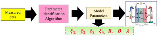
Figure 3.
A diagrammatic representation of the various approaches used in estimating a cell’s unknown parameters.
4. Bald Eagle Search Algorithm
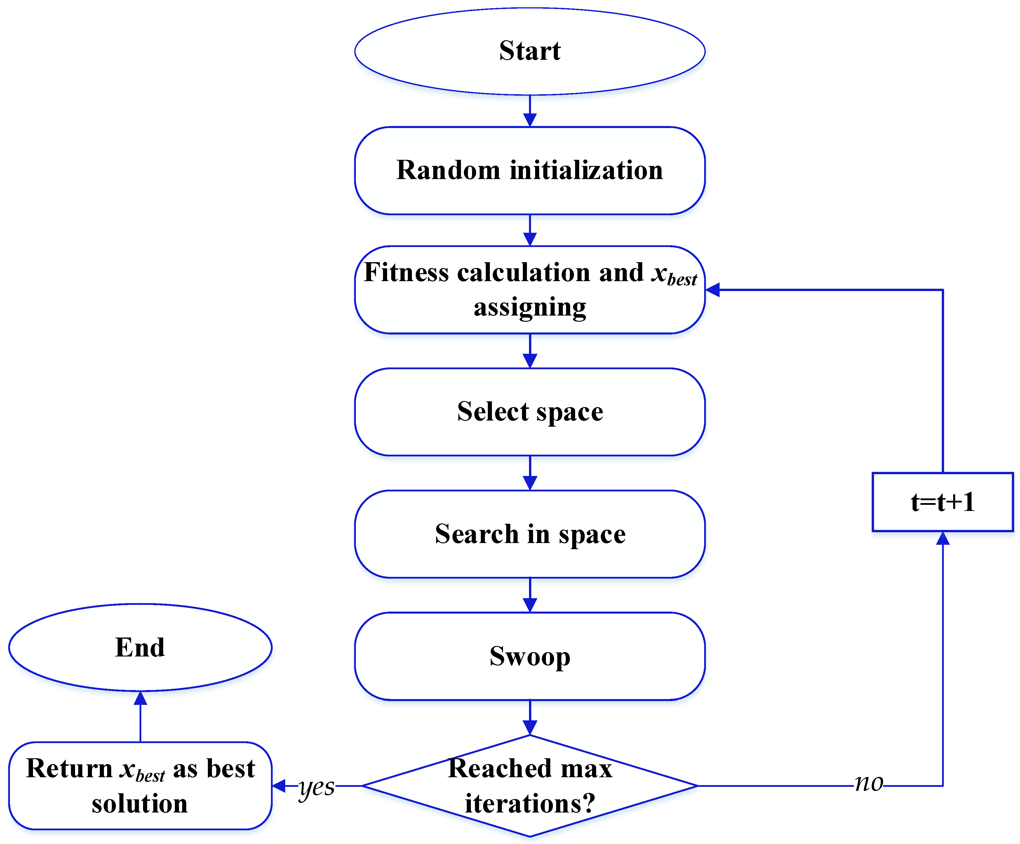
The BES algorithm is an efficient heuristic search algorithm that uses a combination of depth-first and best-first searches. It works by first expanding a node according to the best-first search, then exploring each branch in the deepest possible manner. This algorithm has been found to be effective for a range of applications, such as finding paths in graphs and solving mazes. The algorithm involves three stages: selecting the space with the most potential prey, searching within that space, and swooping from the best-found position to an optimal hunting spot. The first stage is modeled as follows:
where α is a constant [1.5, 2], and r is a random value. The second stage can be modeled as follows:
where X and Y are directional coordinates, calculated as follows:
where β1 is a constant [5, 10], and R is a constant gain [0.5, 2]. The last stage can be expressed as follows:
The BES flowchart is illustrated in Figure 4.
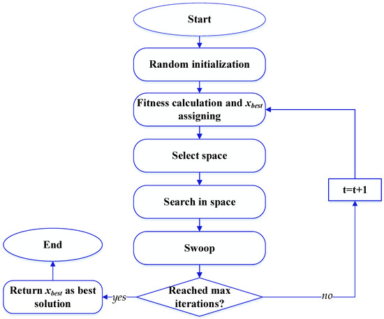
Figure 4.
BES flowchart.
5. Experimental Procedure
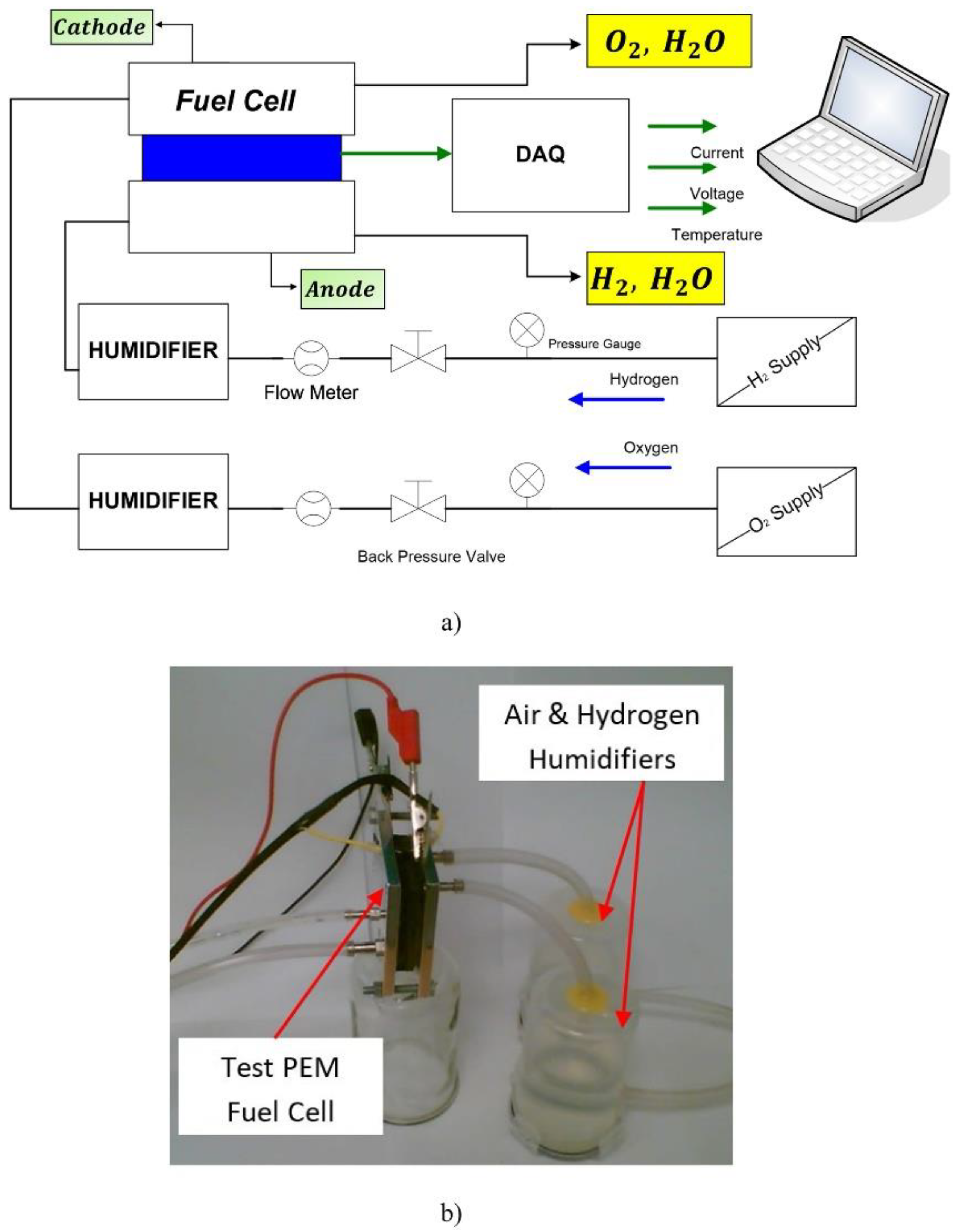
Avista SR–12 PEMFC is considered in this work. The current deduced from the cell varied between 0 and 34 A, and the variation in terms of voltage was between 23 and 43 VDC. The fuel for the cell was passed through an in-house-developed chamber to ensure the hydrogen gas was humidified before entering the cell. This step was critical in ensuring the membrane was well-humidified to allow an increase in protonic conductivity but a reduction in resistance to the electrolyte. Attached to the cell is also a boost converter and a battery, as well as a load cell. The hydrogen gas entering the cell was varied in terms of pressure and flow rate (Figure 5a) to ensure the determination of the effect of the operating conditions on the overall cell performance. The cell was made up of 48 cells, with the active area denoted as 62.5 cm2. The highest cell current was 42 A, while the stack temperature varied between 65 and 80 °C. The cell stacks were cooled using air (Figure 5a,b).

Figure 5.
(a) Experimental setup schematic and (b) in–house-built humidification chamber.
6. Results and Discussion
The optimal parameters of an SR-12 PEM FC have been defined by using five recent optimization methods, namely, bald eagle search algorithm (BES), equilibrium optimizer (EO), coot algorithm (COOT), antlion optimizer (ALO), and heap-based optimizer (HBO). The laptop specifications were HP OMEN 17, Core i9, 32 GB, 1 TB SSD. The simulations were performed using MATLAB software version 2020a. The specifications of SR-12 PEM 500 are shown in Table 1.

Table 1.
The specifications of SR-12 PEM 500.
In order to guarantee an equal comparison, the number of populations was kept at 25, while the maximum number of iterations (nmax) was selected as 250 and 500 to show the effect of the number of iterations on the algorithms’ performance. The maximum and minimum limits of the unknown parameters are outlined in Table 2. Table 3 shows the optimal values of the PEMFC parameters after 30 runs. The absolute error for the obtained parameters using different methods compared to BES is presented in Table A1. The results were evaluated statistically, as shown in Table 4.
Table 2.
Maximum and minimum limits of the parameters.
Table 3.
Optimal values of the PEMFC model parameters using different optimization methods.
Table 4.
Statistical assessments for the considered optimization algorithms.
Considering Table 4, with a maximum number of 500 iterations, the mean cost function values range from 0.035102 to 0.056021. The minimum mean cost function value of 0.035102 is obtained by BES, followed by COOT (0.04155), whereas the largest mean cost function value of 0.056021 is obtained by HBO. The standard deviation values range between 1.15 × 10⁻⁵ and 0.019082. The minimum standard deviation value of 1.15 × 10⁻⁵ is achieved by BES, followed by COOT (0.006312), whereas the largest standard deviation value of 0.019082 is obtained by HBO. In the case of a maximum number of 250 iterations, the mean cost function values range from 0.035794 to 0.089071. The minimum mean cost function value of 0.035794 is obtained by BES, followed by ALO (0.04758), whereas the largest mean cost function value of 0.089071 is obtained by HBO. The standard deviation values range between 0.001557 and 0.045321. The minimum standard deviation value of 0.001557 is achieved by BES, followed by ALO (0.010739), whereas the largest standard deviation value of 0.045321 is obtained by HBO. So, BES is better than ALO, EO, COOT, and HBO. The details of the objective function values for the different algorithms throughout 30 runs is demonstrated in Table 5.
Table 5.
Objective function values for the different algorithms throughout 30 runs.
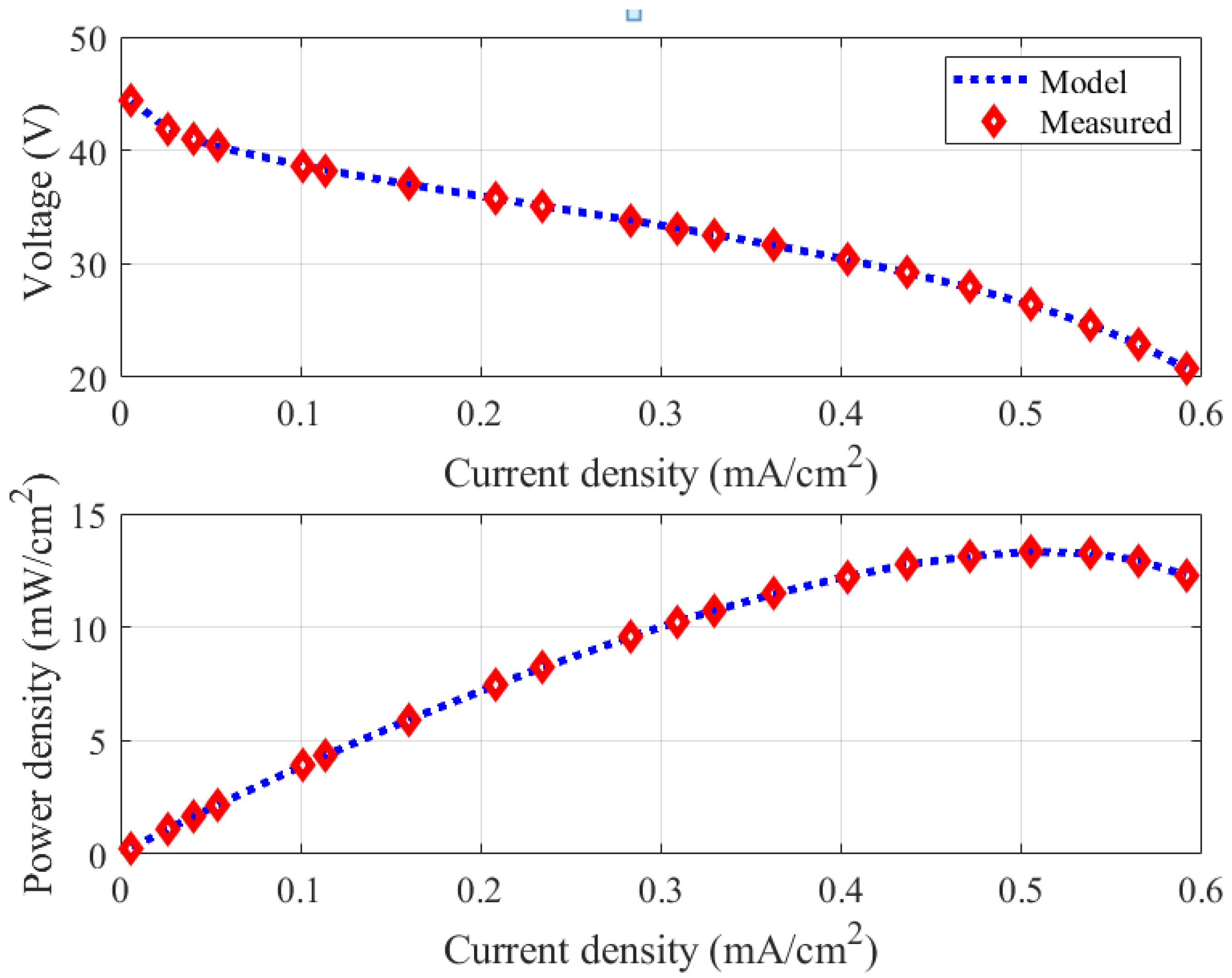
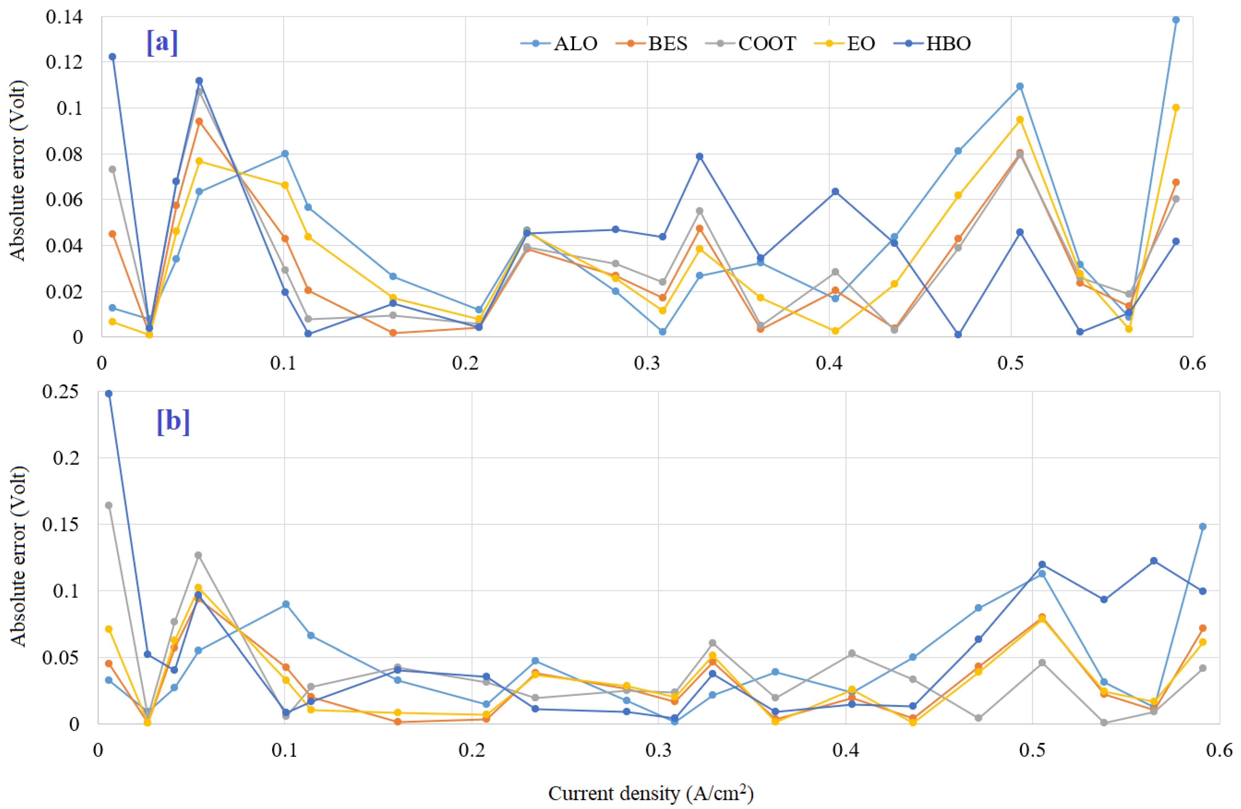
Figure 6 shows the current density, voltage, and power characteristics of the PEMFC using BES. There is an excellent agreement between the estimated and measured data. This proves the superiority of the BES in determining the unknown parameters of the PEMFC. The absolute error in the cell voltage with different optimization algorithms is presented in Table 6 and Figure 7. For the first run with 500 iterations, as presented in Table 5 and Table 6, the SSE values range from 0.0351 to 0.06104. The minimum SSE value of 0.0351 is obtained using the BES, followed by COOT (0.0419), whereas the worst SSE of 0.06104 is obtained by ALO. The best MAE of 0.03251 is obtained by BES, and the worst MAE of 0.04247 is obtained by ALO. Referring to Figure 7a, the maximum absolute error of 0.13831 is obtained by ALO. In the case of the first run with 250 iterations, as demonstrated in Table 5 and Table 6, the SSE values range from 0.03559 to 0.06954. The minimum SSE value of 0.03559 is obtained using the BES, followed by EO (0.03907), whereas the worst SSE of 0.06104 is obtained by ALO. The best MAE of 0.03251 is obtained by BES, and the worst MAE of 0.06954 is obtained by ALO. Referring to Figure 7b, the maximum absolute error of 0.24777 is obtained by HBO.
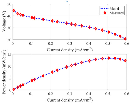
Figure 6.
Current density, voltage, and power characteristics of the PEMFC using BES.
Table 6.
Absolute error in the cell voltage with different optimization algorithms.
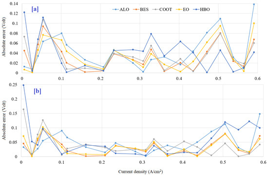
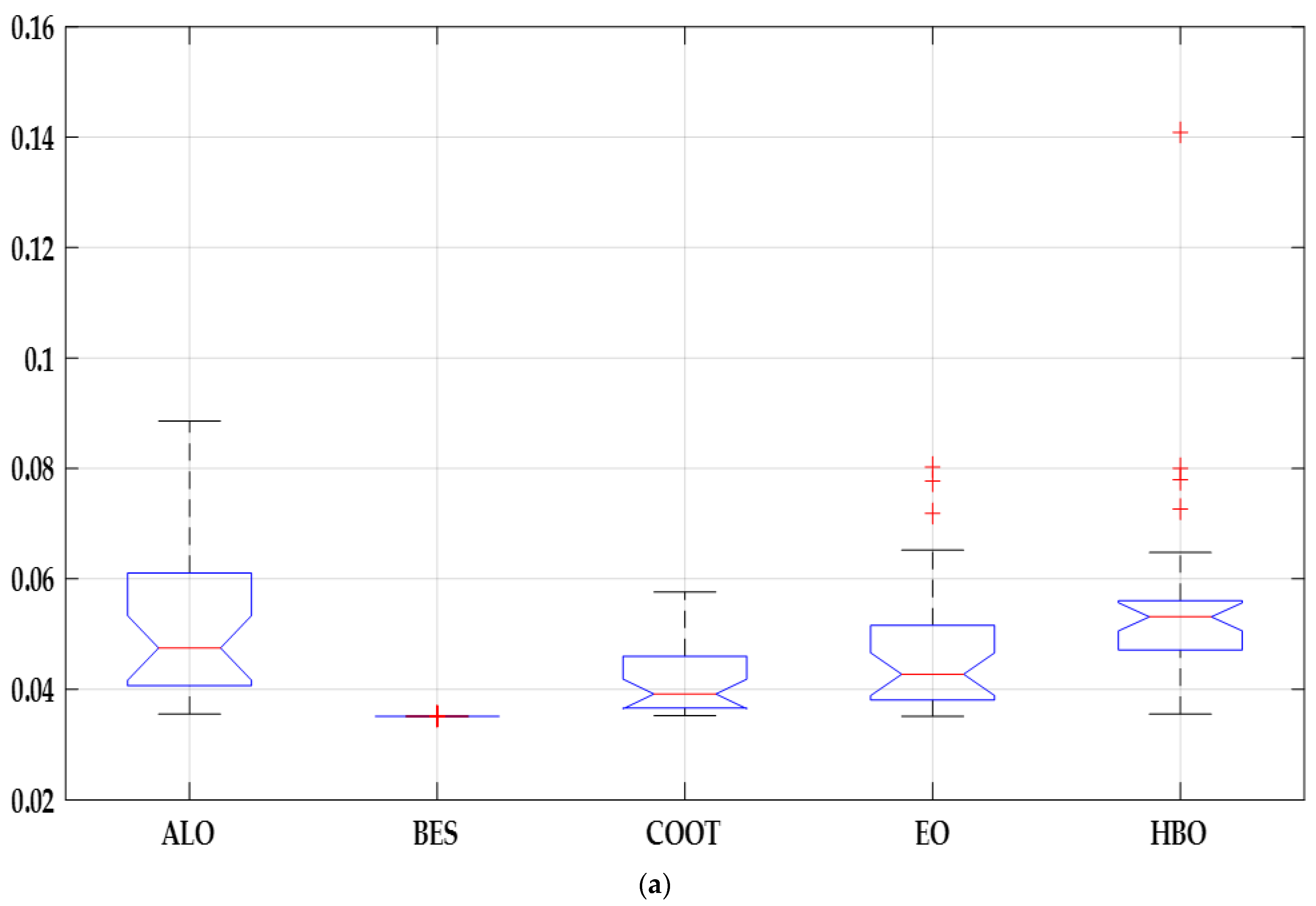
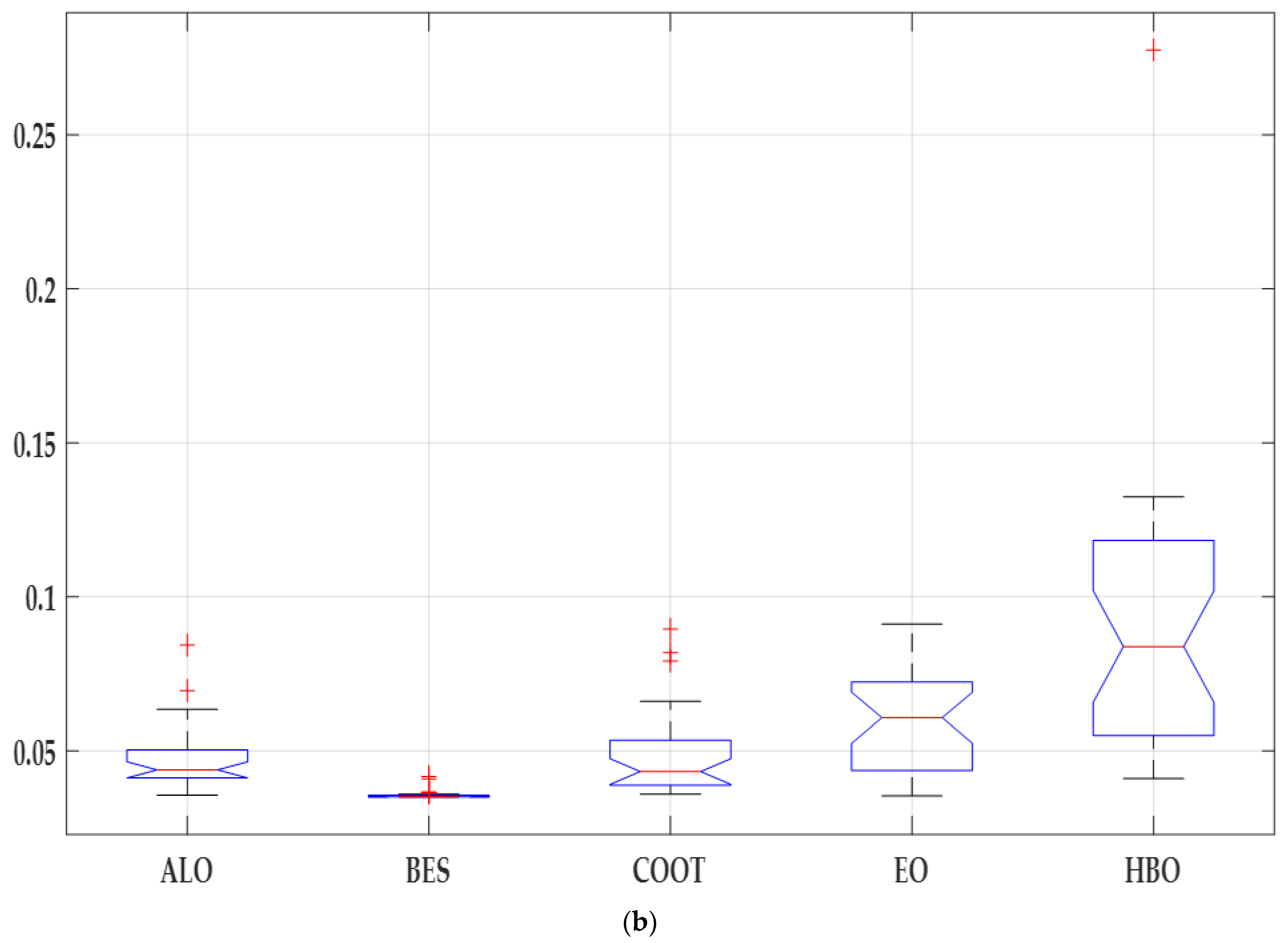
Figure 7.
Absolute error in the cell voltage with different optimization algorithms: (a) nmax 500; (b) nmax 250.
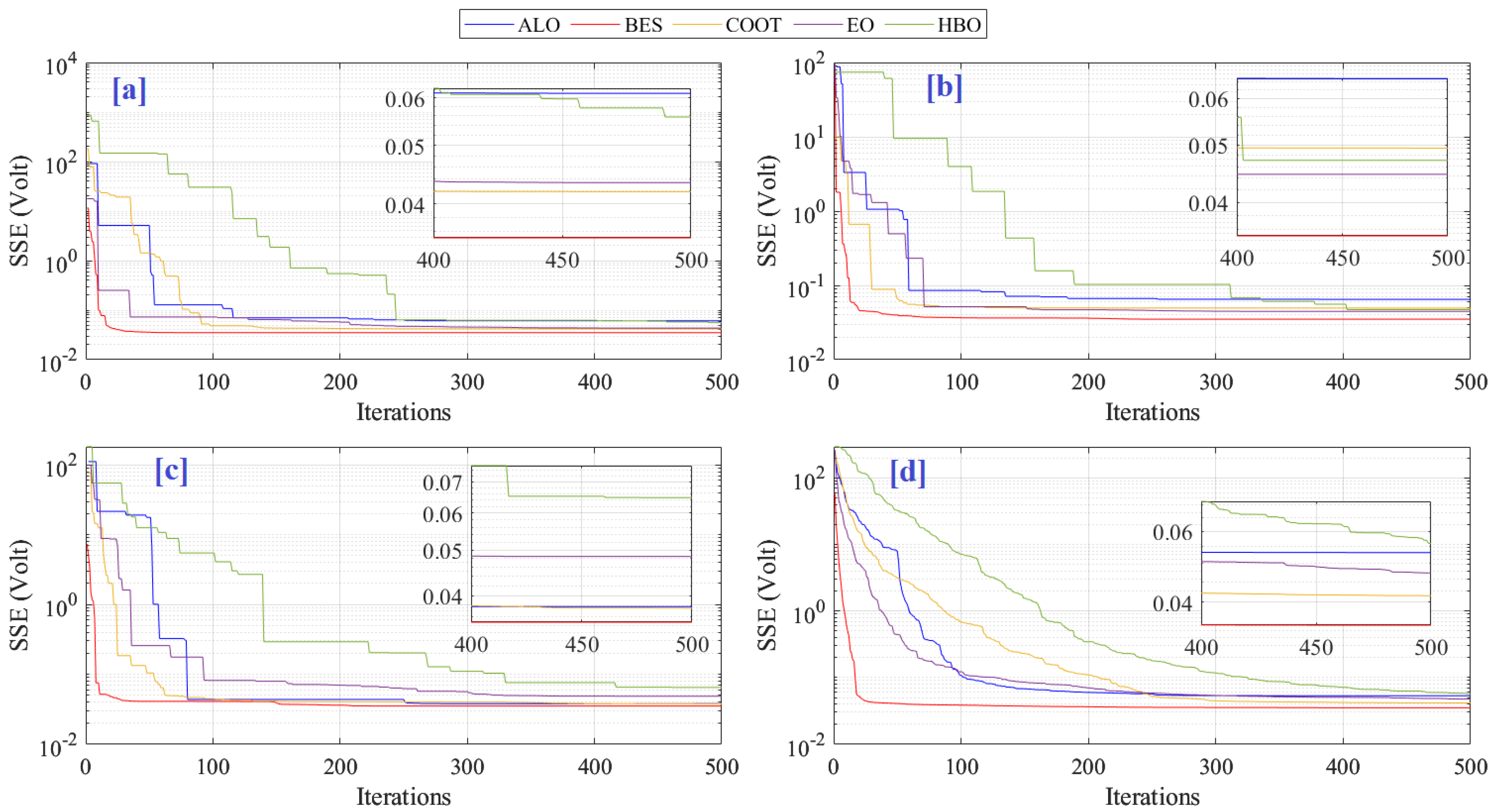
Figure 8 and Figure 9 demonstrate the objective function variation with 500 and 250 iterations, respectively. As demonstrated in Figure 8a and Table 5, for the first run with 500 iterations, the SSE values converge to 0.061045, 0.035099, 0.041897, 0.043371, and 0.061045, respectively, for ALO, BES, COOT, EO, and HBO. BES catches the optimal solution rapidly, whereas HBO needs more time to reach its best solution. During Run 14, as demonstrated in Figure 8b and Table 5, the SSE values converge to 0.069544, 0.03559, 0.066005, 0.039074, and 0.069544, respectively, for ALO, BES, COOT, EO, and HBO. BES catches the optimal solution rapidly, whereas for the second time, HBO needs more time to reach its best solution.
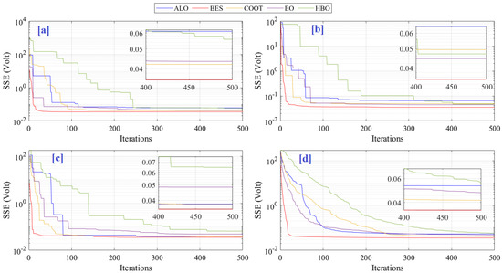
Figure 8.
Objective function variation with 500 iterations: (a) Run 1, (b) Run 14, (c) Run 30, and (d) the average of 30 runs.
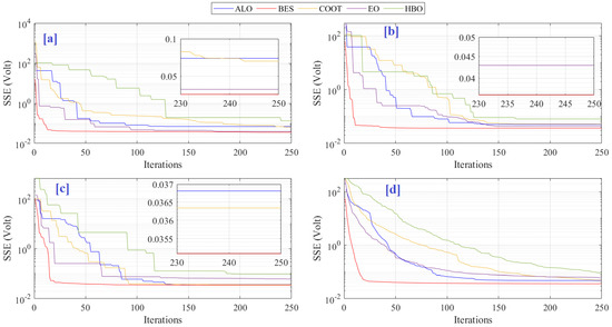
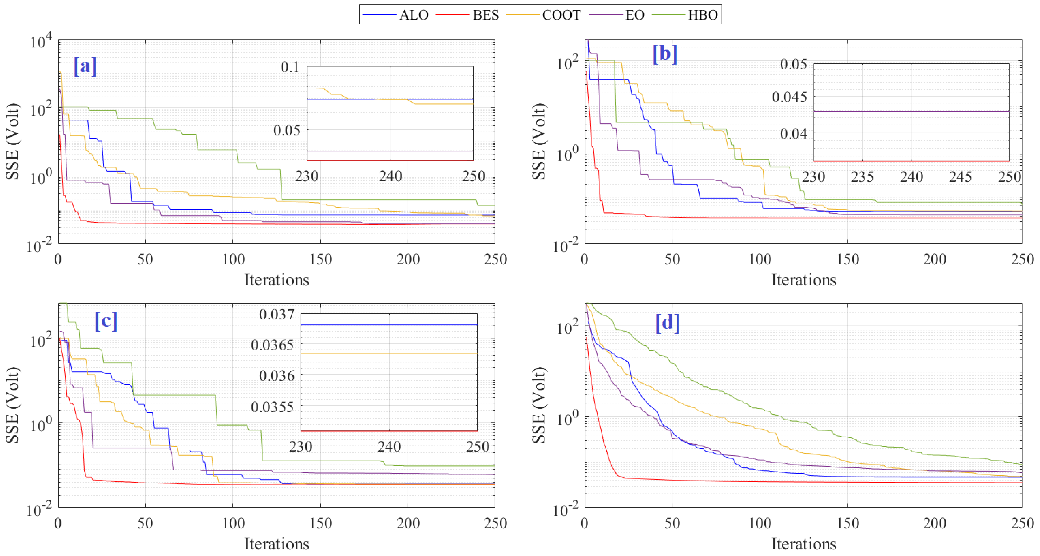
Figure 9.
Objective function variation with 250 iterations: (a) Run 1, (b) Run 14, (c) Run 30, and (d) the average of 30 runs.
ANOVA and Tukey tests were conducted to support the investigation. An ANOVA test is a statistical method used to compare two or more groups. This test measures the mean differences between groups, providing an assessment of how likely each observed difference is to have arisen by random chance. An ANOVA helps answer the question of whether the difference between the means of two or more samples is statistically significant. It works by comparing the variability between groups and the variability within groups to determine whether the differences between group means could have arisen by chance. Table 7 gives the ANOVA test results, and Figure 10 illustrates the corresponding ranking. The BES algorithm can deliver the best performance regarding mean fitness and variations, as demonstrated by Figure 10.
Table 7.
ANOVA test results.
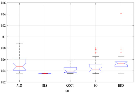

Figure 10.
ANOVA ranking: (a) nmax 500 and (b) nmax 250.
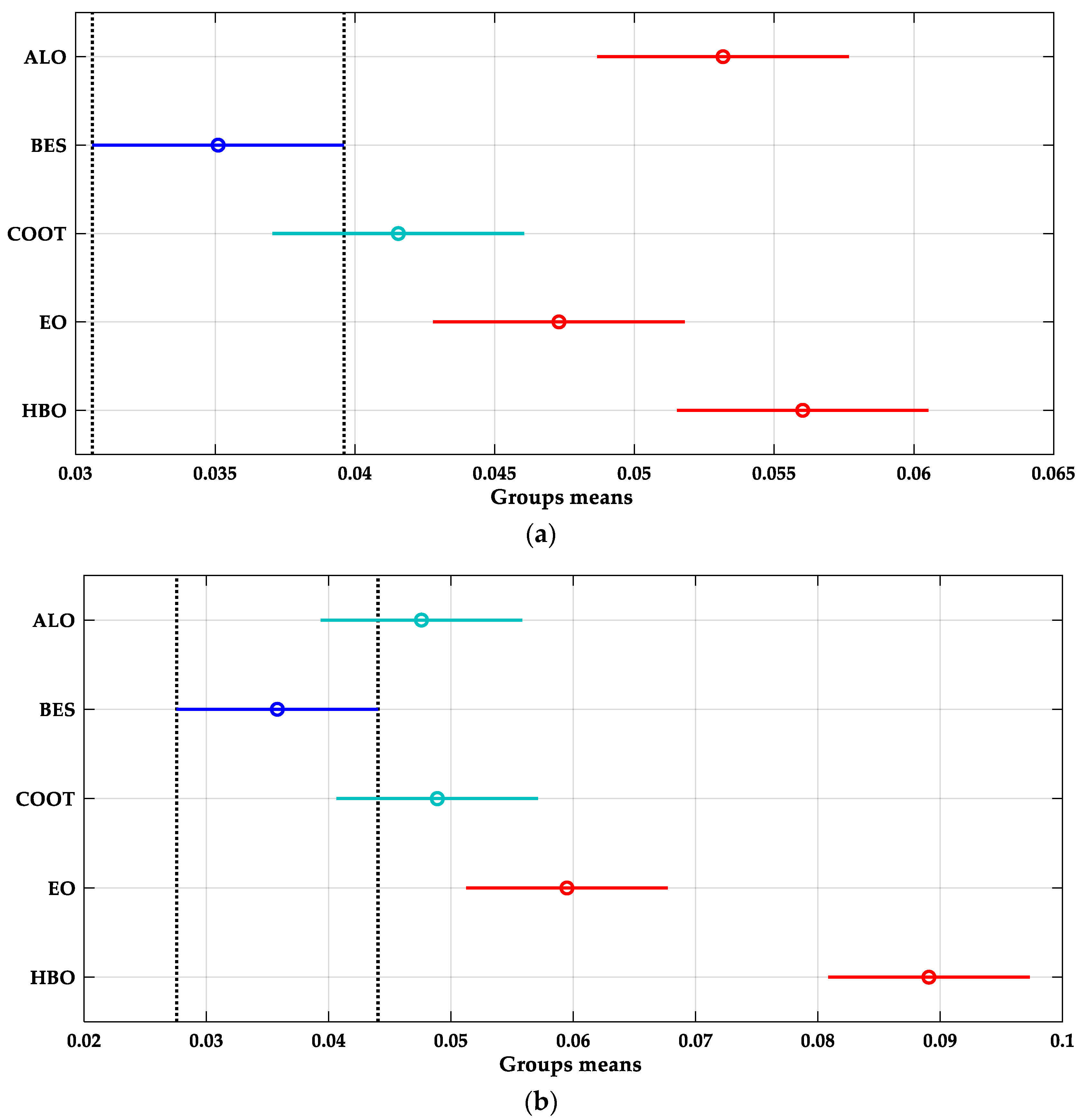
The Tukey test is a statistical procedure used to compare the means of two or more independent samples or datasets. It is a type of post hoc test that takes into account the similarity of group means when evaluating the differences between them. The test is based on the assumption that all datasets have the same variance and that their distribution can be approximated by a normal distribution. It is a powerful tool for detecting significant differences between groups.
The Tukey HSD test, as shown in Figure 11, was performed to approve the two types of ANOVA test results. The ALO, EO, and HBO groups significantly differ from BES for the first case. The COOT mean results indicate that the COOT can provide the second-best results. For the second case, two groups (EO and HBO) have means significantly different from BES, whereas ALO and COOT can provide near performance. However, the BES algorithm offers the best performance for the two cases. The ultimate results of the BES confirm that it can effectively solve this issue.
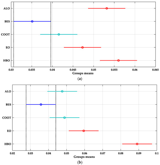
Figure 11.
Tukey test results: (a) nmax 500 and (b) nmax 250.
7. Conclusions
The optimal parameter identification process of the SR–12 PEM fuel-cell model has been investigated in this research work using different recent optimization algorithms. Five optimization methods, namely, bald eagle search algorithm (BES), equilibrium optimizer (EO), coot algorithm (COOT), antlion optimizer (ALO), and heap-based optimizer (HBO), have been considered. Two different numbers of iterations were chosen: 250 and 500. With a 500 maximum number of iterations, the mean cost function values ranged from 0.035102 to 0.056021. The minimum mean cost function value of 0.035102 was obtained by BES, followed by COOT (0.04155), whereas the largest mean cost function value of 0.056021 was obtained by HBO. The standard deviation values ranged between 1.15 × 10⁻⁵ and 0.019082. The minimum standard deviation value of 1.15 × 10⁻⁵ was achieved by BES, followed by COOT (0.006312), whereas the largest standard deviation value of 0.019082 was obtained by HBO. From the data gathered, it can be deduced that the BES predicts results more accurately using the SSE as an objective function and ensures that convergence is attained at a faster rate compared to the other metaheuristic algorithms under investigation; hence, it is suitable for finding solutions to global optimization problems aside from fuel cells. The present study is, however, aimed at providing technical information in relation to the commercialization of fuel cells via the development of digital twins through accurate predictive modeling in the absence of seven unknown parameters; hence, it could be an accurate reference source for the fuel-cell research community and policy makers in the modeling and simulation of fuel cells for the automotive industry and portable and stationary applications. In future work, the validation of the proposed method will be evaluated under the different operating conditions of a PEM fuel cell.
Author Contributions
Conceptualization, H.R., T.W., M.A.A. and E.T.S.; methodology, R.M.G.; software, H.R.; validation, A.G.O., T.W. and M.A.A.; formal analysis, H.R.; investigation, A.G.O.; resources, T.W.; data curation, M.A.A.; writing—original draft preparation, H.R.; writing—review and editing, T.W.; visualization, H.R.; supervision, H.R.; project administration, A.G.O. All authors have read and agreed to the published version of the manuscript.
Funding
Princess Nourah bint Abdulrahman University Researchers Supporting Project number (PNURSP2023R138), Princess Nourah bint Abdulrahman University, Riyadh, Saudi Arabia.
Data Availability Statement
Data will be made available on request.
Acknowledgments
We acknowledge the support from Princess Nourah bint Abdulrahman University Researchers Supporting Project number (PNURSP2023R138), Princess Nourah bint Abdulrahman University, Riyadh, Saudi Arabia.
Conflicts of Interest
The authors declare no conflict of interest.
Appendix A
Table A1.
Absolute error for the obtained parameters using different methods compared to BES.
References
- Ali, M.N.; Mahmoud, K.; Lehtonen, M.; Darwish, M.M.F. Promising MPPT methods combining metaheuristic, fuzzy-logic and ANN techniques for grid-connected photovoltaic. Sensors 2021, 21, 1244. [Google Scholar] [CrossRef] [PubMed]
- Yuan, X.; Liu, Y.; Bucknall, R. A novel design of a solid oxide fuel cell-based combined cooling, heat and power residential system in the U. K. IEEE Trans. Ind. Appl. 2021, 57, 805–813. [Google Scholar] [CrossRef]
- Ihonen, J.; Koski, P.; Pulkkinen, V.; Keränen, T.; Karimäki, H.; Auvinen, S.; Nikiforow, K.; Kotisaari, M.; Tuiskula, H.; Viitakangas, J. Operational experiences of PEMFC pilot plant using low grade hydrogen from sodium chlorate production process. Int. J. Hydrogen Energy 2017, 42, 27269–27283. [Google Scholar] [CrossRef]
- Qiu, Y.; Wu, P.; Miao, T.; Liang, J.; Jiao, K.; Li, T.; Lin, J.; Zhang, J. An intelligent approach for contact pressure optimization of PEM fuel cell gas diffusion layers. Appl. Sci. 2020, 10, 4194. [Google Scholar] [CrossRef]
- Ahmed, K.; Farrok, O.; Rahman, M.M.; Ali, M.S.; Haque, M.M.; Azad, A.K. Proton exchange membrane hydrogen fuel cell as the grid connected power generator. Energies 2020, 13, 6679. [Google Scholar] [CrossRef]
- Nikiforow, K.; Pennanen, J.; Ihonen, J.; Uski, S.; Koski, P. Power ramp rate capabilities of a 5 kW proton exchange membrane fuel cell system with discrete ejector control. J. Power Sources 2018, 381, 30–37. [Google Scholar] [CrossRef]
- Menesy, A.S.; Sultan, H.M.; Korashy, A.; Banakhr, F.A.; Ashmawy, M.G.; Kamel, S. Effective parameter extraction of different polymer electrolyte membrane fuel cell stack models using a modified artificial ecosystem optimization algorithm. IEEE Access 2020, 8, 31892–31909. [Google Scholar] [CrossRef]
- Tanveer, W.H.; Rezk, H.; Nassef, A.; Abdelkareem, M.A.; Kolosz, B.; Karuppasamy, K.; Aslam, J.; Gilani, S.O. Improving fuel cell performance via optimal parameters identification through fuzzy logic based-modeling and optimization. Energy 2020, 204, 117976. [Google Scholar] [CrossRef]
- Sundén, B. Fuel cell types—Overview. In Hydrogen, Batteries and Fuel Cells; Sundén, B., Ed.; Academic Press: Cambridge, MA, USA, 2019; pp. 123–144. [Google Scholar] [CrossRef]
- Fathy, A.; Rezk, H. Multi-verse optimizer for identifying the optimal parameters of PEMFC model. Energy 2018, 143, 634–644. [Google Scholar] [CrossRef]
- Ashraf, H.; Abdellatif, S.O.; Elkholy, M.M.; El-Fergany, A.A. Computational techniques based on artificial intelligence for extracting optimal parameters of PEMFCs: Survey and insights. Arch. Comput. Methods Eng. 2022, 29, 3943–3972. [Google Scholar] [CrossRef]
- Rezk, H.; Olabi, A.G.; Sayed, E.; Wilberforce, T. Role of Metaheuristics in Optimizing Microgrids Operating and Management Issues: A Comprehensive Review. Sustainability 2023, 15, 4982. [Google Scholar] [CrossRef]
- Zhu, Y.; Yousefi, N. Optimal parameter identification of PEMFC stacks using adaptive sparrow search algorithm. Int. J. Hydrogen Energy 2021, 46, 9541–9552. [Google Scholar] [CrossRef]
- Yousri, D.; Mirjalili, S.; Machado, J.T.; Thanikanti, S.B.; Fathy, A.; Elbaksawi, O. Efficient fractional-order modified Harris Hawks optimizer for proton exchange membrane fuel cell modeling. Eng. Appl. Artif. Intell. 2021, 100, 104193. [Google Scholar] [CrossRef]
- Yuan, Z.; Wang, W.; Wang, H.; Yildizbasi, A. Developed coyote optimization algorithm and its application to optimal parameters estimation of PEMFC model. Energy Rep. 2020, 6, 1106–1117. [Google Scholar] [CrossRef]
- Bao, S.; Ebadi, A.; Toughani, M.; Dalle, J.; Maseleno, A.; Baharuddin; Yıldızbası, A. A new method for optimal parameters identification of a PEMFC using an improved version of monarch butterfly optimization algorithm. Int. J. Hydrogen Energy 2020, 45, 17882–17892. [Google Scholar] [CrossRef]
- Abdel-Basset, M.; Mohamed, R.; El-Fergany, A.; Chakrabortty, R.K.; Ryan, M.J. Adaptive and efficient optimization model for optimal parameters of proton exchange membrane fuel cells: A comprehensive analysis. Energy 2021, 233, 121096. [Google Scholar] [CrossRef]
- Wilberforce, T.; Rezk, H.; Olabi, A.G.; Epelle, E.I.; Abdelkareem, M.A. Comparative analysis on parametric estimation of a PEM fuel cell using metaheuristics algorithms. Energy 2023, 262 Pt B, 125530. [Google Scholar] [CrossRef]
- Fathy, A.; Elaziz, M.A.; Alharbi, A.G. A novel approach based on hybrid vortex search algorithm and differential evolution for identifying the optimal parameters of PEM fuel cell. Renew. Energy 2020, 146, 1833–1845. [Google Scholar] [CrossRef]
- Yuan, Z.; Wang, W.; Wang, H. Optimal parameter estimation for PEMFC using modified monarch butterfly optimization. Int. J. Energy Res. 2020, 44, 8427–8441. [Google Scholar] [CrossRef]
- Diab, A.A.Z.; Ali, H.; Abdul-Ghaffar, H.; Abdelsalam, H.A.; Abd El Sattar, M. Accurate parameters extraction of PEMFC model based on metaheuristics algorithms. Energy Rep. 2021, 7, 6854–6867. [Google Scholar] [CrossRef]
- Gupta, J.; Nijhawan, P.; Ganguli, S. Optimal parameter estimation of PEM fuel cell using slime mould algorithm. Int. J. Energy Res. 2021, 45, 14732–14744. [Google Scholar] [CrossRef]
- Qin, F.; Liu, P.; Niu, H.; Song, H.; Yousefi, N. Parameter estimation of PEMFC based on improved fluid search optimization algorithm. Energy Rep. 2020, 6, 1224–1232. [Google Scholar] [CrossRef]
- Yang, B.; Li, D.; Zeng, C.; Chen, Y.; Guo, Z.; Wang, J.; Shu, H.; Yu, T.; Zhu, J. Parameter extraction of PEMFC via Bayesian regularization neural network based meta-heuristic algorithms. Energy 2021, 228, 120592. [Google Scholar] [CrossRef]
- Yuan, Z.; Wang, W.; Wang, H.; Razmjooy, N. A new technique for optimal estimation of the circuit-based PEMFCs using developed Sunflower Optimization Algorithm. Energy Rep. 2020, 6, 662–671. [Google Scholar] [CrossRef]
- Sun, S.; Su, Y.; Yin, C.; Jermsittiparsert, K. Optimal parameters estimation of PEMFCs model using converged moth search algorithm. Energy Rep. 2020, 6, 1501–1509. [Google Scholar] [CrossRef]
- Chen, Y.; Pi, D.; Wang, B.; Chen, J.; Xu, Y. Bi-subgroup optimization algorithm for parameter estimation of a PEMFC model. Expert Syst. Appl. 2022, 196, 116646. [Google Scholar] [CrossRef]
- Syah, R.; Isola, L.A.; Guerrero, J.W.G.; Suksatan, W.; Sunarsi, D.; Elveny, M.; Alkaim, A.F.; Thangavelu, L.; Aravindhan, S. Optimal parameters estimation of the PEMFC using a balanced version of Water Strider Algorithm. Energy Rep. 2021, 7, 6876–6886. [Google Scholar] [CrossRef]
- Guo, H.; Tao, H.; Salih, S.Q.; Yaseen, Z.M. Optimized parameter estimation of a PEMFC model based on improved grass fibrous root optimization algorithm. Energy Rep. 2020, 6, 1510–1519. [Google Scholar] [CrossRef]
- Özdemir, M.T. Optimal parameter estimation of polymer electrolyte membrane fuel cells model with chaos embedded particle swarm optimization. Int. J. Hydrogen Energy 2021, 46, 16465–16480. [Google Scholar] [CrossRef]
- Mossa, M.A.; Kamel, O.M.; Sultan, H.M.; Diab, A.A.Z. Parameter estimation of PEMFC model based on Harris Hawks’ optimization and atom search optimization algorithms. Neural Comput. Appl. 2021, 33, 5555–5570. [Google Scholar] [CrossRef]
- Rezk, H.; Ferahtia, S.; Djeroui, A.; Chouder, A.; Houari, A.; Machmoum, M.; Abdelkareem, M.A. Optimal parameter estimation strategy of PEM fuel cell using gradient-based optimizer. Energy 2022, 239, 122096. [Google Scholar] [CrossRef]
- Zhang, G.; Xiao, C.; Razmjooy, N. Optimal parameter extraction of PEM fuel cells by meta-heuristics. Int. J. Ambient Energy 2020, 43, 2510–2519. [Google Scholar] [CrossRef]
- Han, W.; Li, D.; Yu, D.; Ebrahimian, H. Optimal parameters of PEM fuel cells using chaotic binary shark smell optimizer. Energy Sources A Recov. Util. Environ. Eff. 2019, 1–15. [Google Scholar] [CrossRef]
- Fathy, A.; Babu, T.S.; Abdelkareem, M.A.; Rezk, H.; Yousri, D. Recent approach based heterogeneous comprehensive learning archimedes optimization algorithm for identifying the optimal parameters of different fuel cells. Energy 2022, 248, 123587. [Google Scholar] [CrossRef]
- Yuan, Z.; Wang, W.; Wang, H.; Ashourian, M. Parameter identification of PEMFC based on convolutional neural network optimized by balanced deer hunting optimization algorithm. Energy Rep. 2020, 6, 1572–1580. [Google Scholar] [CrossRef]
- Sultan, H.M.; Menesy, A.S.; Kamel, S.; Hasanien, H.M.; Al-Durra, A. Identifying optimal parameters of proton exchange membrane fuel cell using water cycle algorithm. In Proceedings of the 2020 2nd International Conference on Smart Power & Internet Energy Systems, Bangkok, Thailand, 15–18 September 2020; pp. 176–181. [Google Scholar]
- Alsaidan, I.; Shaheen, M.A.; Hasanien, H.M.; Alaraj, M.; Alnafisah, A.S. A PEMFC model optimization using the enhanced bald eagle algorithm. Ain Shams Eng. J. 2022, 13, 101749. [Google Scholar] [CrossRef]
- Abaza, A.; El-Sehiemy, R.A.; Mahmoud, K.; Lehtonen, M.; Darwish, M.M. Optimal estimation of proton exchange membrane fuel cells parameter based on coyote optimization algorithm. Appl. Sci. 2021, 11, 2052. [Google Scholar] [CrossRef]
- Blanco-Cocom, L.; Botello-Rionda, S.; Ordoñez, L.; Valdez, S.I. Robust parameter estimation of a PEMFC via optimization based on probabilistic model building. Math. Comput. Simul. 2021, 185, 218–237. [Google Scholar] [CrossRef]
- Lu, X.; Kanghong, D.; Guo, L.; Wang, P.; Yildizbasi, A. Optimal estimation of the proton exchange membrane fuel cell model parameters based on extended version of crow search algorithm. J. Clean. Prod. 2020, 272, 122640. [Google Scholar] [CrossRef]
- Menesy, A.S.; Sultan, H.M.; Kamel, S. Extracting model parameters of proton exchange membrane fuel cell using equilibrium optimizer algorithm. In Proceedings of the 2020 International Youth Conference on Radio Electronics, Electrical and Power Engineering, Moscow, Russia, 12–14 March 2020; pp. 1–7. [Google Scholar]
- Duan, B.; Cao, Q.; Afshar, N. Optimal parameter identification for the proton exchange membrane fuel cell using satin bowerbird optimizer. Int. J. Energy Res. 2019, 43, 8623–8632. [Google Scholar] [CrossRef]
- Fathy, A.; Aleem, S.A.; Rezk, H. A novel approach for PEM fuel cell parameter estimation using LSHADE-EpSin optimization algorithm. Int. J. Energy Res. 2021, 45, 6922–6942. [Google Scholar] [CrossRef]
- Isa, Z.M.; Nayan, N.M.; Arshad, M.H.; Kajaan, N.A.M. Optimizing PEMFC model parameters using ant lion optimizer and dragonfly algorithm: A comparative study. Int. J. Electr. Comput. Eng. 2019, 9, 5295. [Google Scholar] [CrossRef]
- Song, Y.; Tan, X.; Mizzi, S. Optimal parameter extraction of the proton exchange membrane fuel cells based on a new Harris Hawks optimization algorithm. Energy Sources A Recov. Util. Environ. Eff. 2020, 1–18. [Google Scholar] [CrossRef]
- Yang, Z.; Liu, Q.; Zhang, L.; Dai, J.; Razmjooy, N. Model parameter estimation of the PEMFCs using improved barnacles mating optimization algorithm. Energy 2020, 212, 118738. [Google Scholar] [CrossRef]
- Sun, X.; Wang, G.; Xu, L.; Yuan, H.; Yousefi, N. Optimal estimation of the PEM fuel cells applying deep belief network optimized by improved archimedes optimization algorithm. Energy 2021, 237, 121532. [Google Scholar] [CrossRef]
- Hasanien, H.M.; Shaheen, M.A.; Turky, R.A.; Qais, M.H.; Alghuwainem, S.; Kamel, S.; Tostado-Véliz, M.; Jurado, F. Precise modeling of PEM fuel cell using a novel enhanced transient search optimization algorithm. Energy 2022, 247, 123530. [Google Scholar] [CrossRef]
- Ćalasan, M.; Aleem, S.H.A.; Hasanien, H.M.; Alaas, Z.M.; Ali, Z.M. An innovative approach for mathematical modeling and parameter estimation of PEM fuel cells based on iterative Lambert W function. Energy 2022, 264, 126165. [Google Scholar] [CrossRef]
- Wilberforce, T.; Olabi, A.G.; Rezk, H.; Abdelaziz, A.Y.; Abdelkareem, M.A.; Sayed, E.T. Boosting the output power of PEM fuel cells by identifying best-operating conditions. Energy Convers. Manag. 2022, 270, 116205. [Google Scholar] [CrossRef]
- Rezk, H.; Wilberforce, T.; Sayed, E.T.; Alahmadi, A.N.M.; Olabi, A.G. Finding best operational conditions of PEM fuel cell using adaptive neuro-fuzzy inference system and metaheuristics. Energy Rep. 2022, 8, 6181–6190. [Google Scholar] [CrossRef]
- Wilberforce, T.; Olabi, A.G.; Monopoli, D.; Dassisti, M.; Sayed, E.T.; Abdelkareem, M.A. Design optimization of proton exchange membrane fuel cell bipolar plate. Energy Convers. Manag. 2023, 277, 116586. [Google Scholar] [CrossRef]
- Ashraf, H.; Abdellatif, S.O.; Elkholy, M.M.; Attia, A. El-Fergany. Honey badger optimizer for extracting the ungiven parameters of PEMFC model: Steady-state assessment. Energy Convers. Manag. 2022, 258, 115521. [Google Scholar] [CrossRef]
- Eelsayed, S.K.; Ahmed, A.; Ehab Ehab Elsayed Elattar, Attia El-Fergany. Steady-state modelling of pem fuel cells using gradient-based optimizer. Dyna 2021, 96, 520–527. [Google Scholar] [CrossRef] [PubMed]


Disclaimer/Publisher’s Note: The statements, opinions and data contained in all publications are solely those of the individual author(s) and contributor(s) and not of MDPI and/or the editor(s). MDPI and/or the editor(s) disclaim responsibility for any injury to people or property resulting from any ideas, methods, instructions or products referred to in the content. |
© 2023 by the authors. Licensee MDPI, Basel, Switzerland. This article is an open access article distributed under the terms and conditions of the Creative Commons Attribution (CC BY) license (https://creativecommons.org/licenses/by/4.0/).