Article

A Fault Diagnosis Algorithm for the Dedicated Equipment Based on the CNN-LSTM Mechanism

1
Key Laboratory of Intelligent Control and Optimization for Industrial Equipment of Ministry of Education, School of Control Science and Engineering, Dalian University of Technology, Dalian 116081, China
2
School of Innovation and Entrepreneurship, Dalian University of Technology, Dalian 116024, China
*
Author to whom correspondence should be addressed.
Energies 2023, 16(13), 5230; https://doi.org/10.3390/en16135230
Submission received: 29 May 2023 / Revised: 3 July 2023 / Accepted: 4 July 2023 / Published: 7 July 2023

Abstract

:
Dedicated equipment, which is widely used in many different types of vehicles, is the core system that determines the combat capability of special vehicles. Therefore, assuring the normal operation of dedicated equipment is crucial. With the increase in battlefield complexity, the demand for equipment functions is increasing, and the complexity of dedicated equipment is also increasing. To solve the problem of fault diagnosis of dedicated equipment, a fault diagnosis algorithm based on CNN-LSTM was proposed in this paper. CNN and LSTM are used in the model adopted by the algorithm to extract spatial and temporal features from the data. CBAM is used to enhance the model’s accuracy in identifying faults for dedicated equipment. Data on dedicated equipment faults were obtained from a hardware-in-loop simulation platform to verify the model. It is demonstrated that the proposed fault diagnosis algorithm has high recognition ability for dedicated equipment by comparing it to other neural network models.

1. Introduction

The amount of intelligence and integration of industrial equipment is increasing as information technology advances, which refines the composition structure of industrial equipment. At the same time, this change also dramatically increases the difficulty regarding fault diagnosis, making the disassembly fault diagnosis method challenging to apply to the current situation. Currently, there are two types of fault diagnosis methods: one is to use mechanism analysis, signal analysis, and so on; the other is to use machine learning and other methods for fault diagnosis. The former method must depend on plenty of prior knowledge for fault diagnosis, so this method has certain limitations in terms of fault diagnosis [1,2,3,4]. For the latter, fault diagnosis is mostly completed via machine learning and other methods. This method of fault diagnosis relies less on prior knowledge, or even does not need prior knowledge.
The first fault diagnosis method mainly uses time–frequency analysis, and mechanism analysis to analyze faults. In Ref. [5], Young et al. applied cepstrum technology to extract bearing fault features and achieved an excellent anti-noise effect. In Ref. [6], Yang et al. combined envelope spectrum analysis and empirical mode decomposition to propose a new fault diagnosis method for rolling bearings. This method carried out envelope spectrum analysis on components after empirical mode decomposition. In Ref. [7], Klausen et al. proposed a fault diagnosis method based on automatic envelope spectrum analysis.
The second fault diagnosis method mainly adopts machine learning methods, such as BP neural network, SVM, etc. In the study of fault diagnosis of dedicated equipment, the fault diagnosis method combining rough set theory and DS evidence theory has produced impressive outcomes [8]. In the research of bearing fault diagnosis, a hybrid framework based on multi-envelope teaching optimization combining variational mode decomposition and support vector machine is proposed, which can achieve good results in bearing fault classification [9]. Due to the poor processing effect of classical machine learning algorithms in the face of processing large amounts of bearing data, a fault diagnosis model based on quantum least squares support vector machine was proposed by Li et al. [10], which combined HHL algorithm in quantum computing with least squares support vector machine algorithm to alleviate the problem effectively.
Machine learning algorithms work well in other areas too. Mansouri et al. [11] combined the improved artificial butterfly optimization algorithm with SVM and applied it in the fault diagnosis research of a wind energy conversion system. Cheng et al. [12] proposed a hybrid intelligent diagnosis method based on improved sine cosine algorithms and BP neural network (ISCA-BP), and experiments proved that the method has good applicability in transformer fault classification. Hu et al. [13] introduced BP neural network into the study of robot joint fault diagnosis. Li et al. [14] proposed a fault diagnosis model combining the decision tree and FCNN and used it to study the fault diagnosis of transformers. Experiments demonstrate the generalizability of this method.
The use of machine learning for fault diagnosis decreases dependence on prior knowledge to a certain extent, and it has made remarkable achievements in the study of fault diagnosis. However, the traditional machine learning method also has certain limitations in the face of complex models or large amounts of data.
The concept of deep learning was put forward in 2006. With the development of information technology, the computing power of computers has increased tremendously, and deep learning has effectively been utilized across many areas, gradually improving people’s lives [15,16,17]. Common network structures in fault diagnosis include deep belief networks (DBN), generative adversarial networks (GAN), recurrent neural networks (RNN), convolutional neural networks (CNN), etc.
(1)
Deep belief network
The DBN belongs to the probabilistic graph model, which is composed of multiple limiting Boltzmann machine layers. Niu et al. [18] proposed an adaptive deep confidence network based on principal component analysis and parameter correction linear element activation layer. The method was used in the fault diagnosis for rolling bearing. Gao et al. [19] studied bearing fault diagnosis using the DBN optimized by the salp swarm algorithm. Tran et al. [20] proposed a fault diagnosis method combining Teager–Kaiser energy operation (TKEO) and the DBN for reciprocating compressor valves. The method used the TKEO to estimate the amplitude envelope and wavelet transform to remove noise. DBN is used to classify faults.
(2)
Generative adversarial network
Generative adversarial network is a generative model that is applied to problems such as data generation and is often used to solve the problem of less labeled training set data. Zhou et al. [21] designed a generator and discriminator of a GAN for the impact of unbalanced data problems on fault diagnosis results and applied them in the study of bearing fault diagnosis. Pham et al. [22] proposed an effective GAN based on data enhancement for the early low-speed fault diagnosis of rolling bearings and proved the effectiveness of the network in the unbalanced composite dataset.
(3)
Recurrent neural network
Different from artificial neural networks, recurrent neural networks can obtain time sequence information in data and have better processing ability for data with strong correlation. Han et al. [23] adopted the method combining a CNN and gated cycle unit to classify faults and applied it to the study of bearing faults. Zhang et al. [24] designed a fault diagnosis method for rotating machinery based on RNN. Firstly, the model input is a two-dimensional image converted by a one-dimensional time series vibration signal. Then, the gated cycle unit is introduced, and the representative features contained in the time sequence data are extracted by using the time information. Finally, the multi-layer perceptron is used for fault identification. LSTM is a special cyclic neural network that is suitable for processing long time sequence information. Jalayer et al. [25] proposed a model combining fast Fourier transform and continuous wavelet transform to obtain fault characteristics of rotating machinery fault information and then used the structure combining CNN and LSTM to classify faults. Compared with the other 12 fault diagnosis models, it is proved that this method has better fault diagnosis accuracy. LSTM has also been applied to fault diagnosis research of wind turbines [26,27] and industrial devices [28].
(4)
Convolutional neural network
Since the CNN was first proposed in 1989 [29], its theory has been developed rapidly. Today, it has become one of the most common deep learning models. The convolutional neural network can effectively extract data features and facilitate fault classification. Sinitsin et al. [30] proposed the CNN-MLP hybrid model for rolling bearing fault diagnosis, which combined mixed input to carry out the fault diagnosis of rolling bearing. Janssens et al. [31] proposed a feature learning method for state monitoring based on CNN to research rotating machinery faults. Experiments proved that the proposed method was superior to the method using manual engineering features and random forest classifiers.
The main contributions of this paper can be summarized as follows:
(1)
Dedicated equipment is the core equipment that determines the normal operation of special vehicles and is widely used in various types of vehicles. In previous studies, due to the difficulty in data acquisition of dedicated equipment, classical machine learning algorithms were mainly adopted. In this paper, fault data were obtained through a simulation platform and the deep learning method was adopted for fault diagnosis research of dedicated equipment.
(2)
This paper presents a fault diagnosis model for dedicated equipment based on CNN-LSTM. LSTM is added to the traditional CNN so that the spatial–temporal features of the data can be extracted. In addition, CBAM is used to enhance the capability of extracting critical features.
(3)
In this paper, the model is trained and verified by using the data of the hardware-in-loop simulation platform of dedicated equipment. By verifying the parameters of the proposed model and analyzing the fault classification process, it is proved that the fault diagnosis model has a good classification effect on the fault problems of dedicated equipment. By comparing with different models, it is proved that the proposed method is a potential solution to the fault diagnosis problem for dedicated equipment.
The rest of this paper is organized as follows: Section 2 briefly introduces CNN, CBAM, and LSTM. Section 3 introduces the proposed model based on LSTM and the fault model training process. In Section 4, the data sources used in this paper are introduced, and the proposed model is analyzed and compared. Conclusions are summarized in Section 5.

2. Theoretical Introduction and Analysis

2.1. Convolutional Neural Network

Convolutional, pooling, and activation layers make up the majority of a CNN. The core of the CNN is the convolutional layer, and the core part of the convolutional layer is the convolution operation. The convolution operation is the inner product of different parts of the data and filter matrix so as to extract the feature information in the data. Different convolution kernels can extract different features from data, and the size of kernels also has an important influence on feature extraction. The two are crucial factors to ensure the convolution layer operates normally as a result.
The mathematical expression of convolution operation is:
x j γ = f i = 0 C 1 x i γ 1 k i j γ + b j γ
γ is the number of the current layer of the neural network, x j γ is the j th eigenmatrix of the current layer, f is the activation function, x i γ 1 is the data element of the γ 1 layer, and C is the number of kernels of input data. k i j γ is the weight matrix of the corresponding convolution kernel; b j γ is the bias matrix.
By adjusting the filter on the input data and choosing the maximum or average value of the data in the sliding window as the output of the pooling unit, the pooling layer can implement the function of downsampling. The activation function ultimately determines whether to send a signal and what to send to the next neuron. The Sigmoid, Tanh, and ReLU activation functions are frequently used activation functions.
Sigmoid
f x = 1 1 + e x
Tanh
f x = e x e x e x + e x = 2 1 + e 2 x 1
ReLU
f x = max 0 , x , x 0 0 , x < 0

2.2. CBAM

CBAM is a lightweight attention module for designing CNN that can be integrated into any CNN structure [32,33]. Compared with other attention mechanisms, CBAM adjusts features by inferring attention weights from two dimensions: space and channel. Therefore, CBAM calculates the attention diagram of the feature graph through two modules. The first module is channel attention module (CAM), and the other is the spatial attention module (SAM). The structure is shown in Figure 1.
The mathematical formula for CBAM’s attention mechanism is as follows:
F = M C F F F = M S F F
where F R C H W is the input of CBAM, M C F R C 1 1 is the output of CAM, and M S F R 1 H W is the output of SAM. The mathematical formula for CAM’s attention mechanism is as follows:
M C ( F ) = σ ( M L P ( A v g P o o l ( F ) ) + M L P ( M a x P o o l ( F ) ) ) = σ ( W 1 ( W 0 ( F a v g c ) ) + W 1 ( W 0 ( F max c ) ) )
The mathematical formula for SAM’s attention mechanism is as follows:
M S F = σ f A v g P o o l F ; M a x P o o l F = σ f F a v g s ; F max s
where W 0 R C / r C , W 1 R C C / r , σ is the activation function, f is the convolution layer whose convolution kernel is 7∗7.

2.3. LSTM

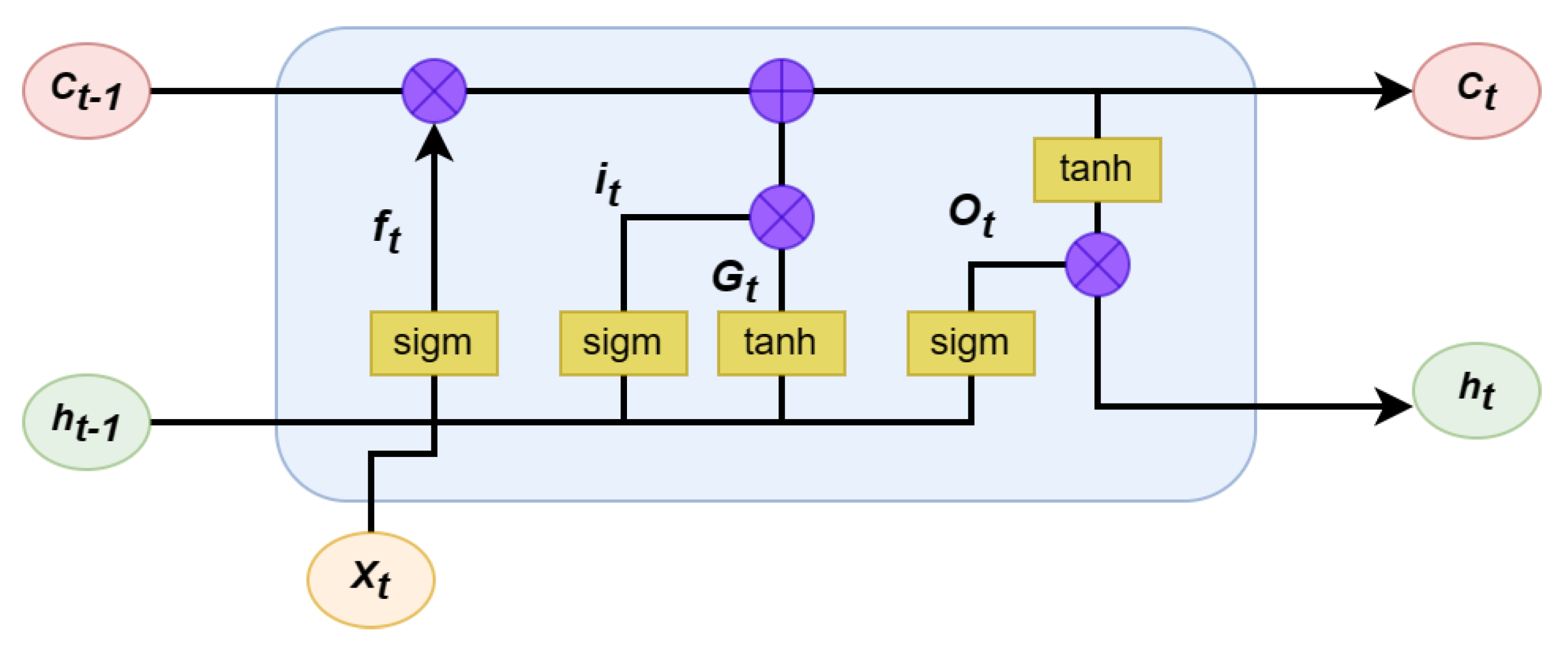
LSTM is a kind of RNN suitable for processing long time sequence information. Compared with traditional RNN, LSTM can deal with long-term dependent data better by adding gate mechanism and cell state. The LSTM’s structure is depicted in Figure 2.
By adding cell state C t , LSTM can store important information for a long time, and this information can be dynamically adjusted as the input changes. The operation of processing information is carried out by the gate mechanism. In Figure 2, they are the memory gate, input gate, and output gate from left to right.
The forgetting door can be calculated using the following formula:
f t = s i g m o i d w f · h t 1 , x t + b f
w f represents the weight matrix, b f represents the bias vector, h t 1 represents the output of the previous unit, and x t represents the current input.
The specific formula of the first stage is shown as follows:
i t = s i g m o i d w i · h t 1 , x t + b i G t = tanh w g · h t 1 , x t + b g
where w g , w i are the weight matrix, and b i , b s is the bias vector. The purpose of this stage is to select the information to be retained. The second stage is to update the cell state. The formula is shown as follows:
C t = C t 1 f t + i t G t
The formula for the output gate is shown as follows:
O t = s i g m o i d w o · h t 1 , x t + b o h t = O tanh C t
where w o and b o are weight matrix and bias vector, respectively.
Since LSTM can effectively process long time sequence information, it still has an excellent solution to the problem of dependence between distant words in natural language processing, except in fault diagnosis research.

3. Fault Diagnosis Model Based on CNN-LSTM

3.1. Fault Diagnosis Model Architecture Based on CNN-LSTM

Since there is a strong correlation between different signals of dedicated equipment and the traditional CNN cannot extract the sequential features in the data, this paper adds LSTM to the traditional CNN to enhance the feature extraction ability. The fault diagnosis model based on CNN-LSTM for dedicated equipment proposed in this paper combines the characteristics of CNN and LSTM to obtain the deep features in the data. Meanwhile, CBAM is used to improve the fault classification effect of dedicated equipment.
The structure diagram of the proposed model is shown in Figure 3. It is primarily separated into four components. Firstly, the convolution layer is used to process the data and extract the features of the data. Then, the time complexity is reduced through the processing of the pooling layer. After that, the spatial–temporal features of the data are extracted through the second and third parts. At the same time, the CBAM mechanism can encourage the model to pay attention to the critical information, which is helpful to the subsequent information extraction and increases the classification accuracy. Finally, the data flow to the last part is extracted by LSTM and expanded into a one-dimensional vector, and then the data are classified by the full connection layer. The parameters of the proposed model are shown in Table 1.

3.2. Fault Model Training Process

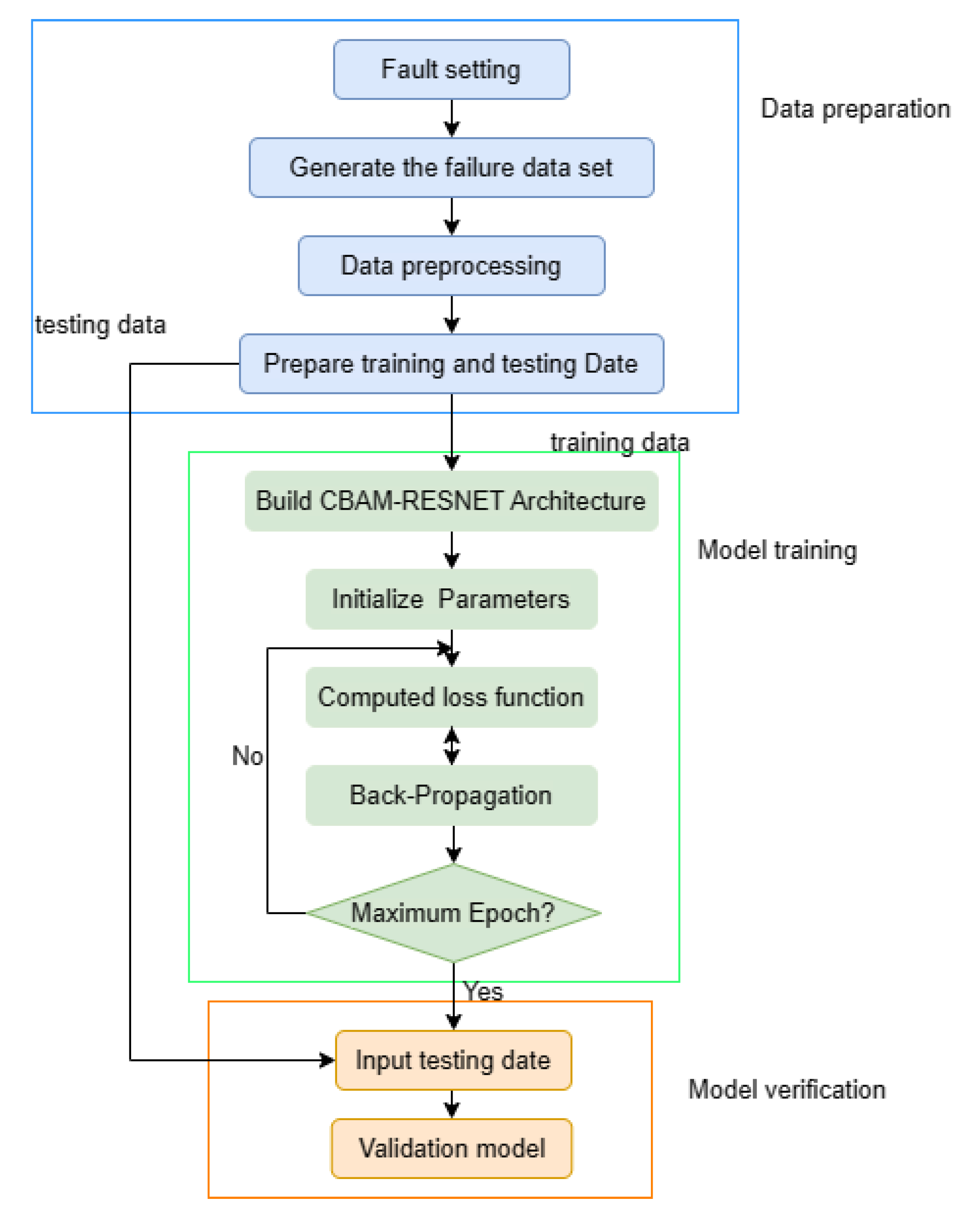
The training flow of dedicated equipment fault diagnosis is shown in Figure 4. Firstly, validation data are obtained from the hardware-in-loop simulation platform of dedicated equipment, and 23 kinds of faults are set using the platform’s fault injection system. For each fault setting, users need to use the platform to perform corresponding operations, such as launch and move commands, so that the collected data contain more comprehensive fault characteristics. After setting a fault, users need to store data. Further, 80 samples were selected for each fault type, and each sample contained 128 data and used all fault types as one dataset. A total of three datasets are stored. After that, the fault data are generated into a file in the specified form.
Then, the data are preprocessed, and 80% of the processed data are taken as the training set and 20% as the test set. After that, the model was trained, and the cross-entropy loss function was utilized to calculate the model’s output. The backpropagation algorithm and Adam algorithm were used to update the parameters. The learning rate was 0.001, the batch size was 32, and the epoch was 1000. Finally, the test set is used to verify the model, including analyzing the classification process of the model, comparing with different fault diagnosis models, etc. Through the verification results, it is judged whether the model meets the requirements.

4. Analysis and Verification

4.1. Fault Data Acquisition and Preprocessing

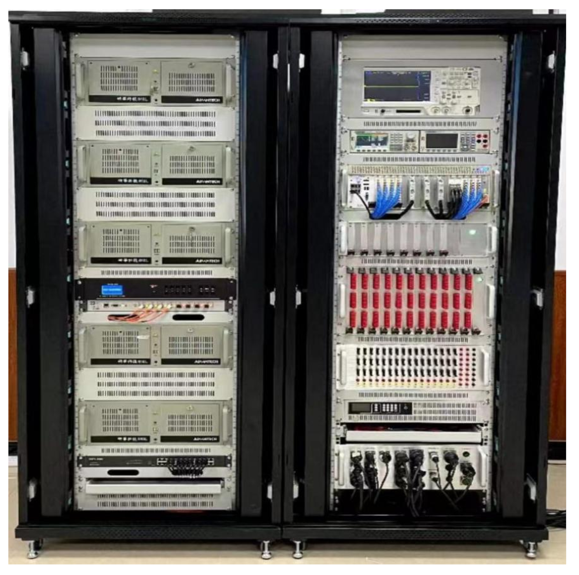
This paper obtains the training and verification data of the proposed model by the hardware-in-loop simulation platform of dedicated equipment. A physical image of the platform is shown in Figure 5. The platform is used to set the required faults, and then operations are performed according to the operational requirements of the dedicated equipment, and the fault data are stored. The fault types studied in this paper are mainly the open circuit of the signal channel of the dedicated equipment. The collected data contain most of the signals received and sent by the dedicated equipment, and the collected signals can contain all the characteristics of the required faults. At the same time, the three datasets used in this paper are stored for the stable operation of the platform. There are 23 fault types studied in this paper, 80 samples were selected for each fault type, each sample contained 128 data, and all fault types were used as one dataset.
Figure 6 shows the numerical changes of some other channel signals when the signal channel of the 26V power pin of the dedicated equipment breaks down. As can be seen from the operating mechanism of the device, when the signal of a channel disappears, the signal of other channels will also change accordingly. As shown in Figure 6, the channel change occurs in various fault types, so the data classification is relatively complicated. At the same time, the data collected by the hardware-in-loop simulation platform are obtained by the acquisition card and related programs. There will be the problem of information distortion, so it is essential to conduct data preprocessing.
Data preprocessing includes removing incomplete and wrong data and screening the data according to the operation mechanism of equipment components, signal characteristics, etc. Some signals of the dedicated equipment are shown in Table 2, and the signal value in Table 2 is the voltage range of the corresponding signal. If the collected signal value is not within the range of the corresponding signal value, the corresponding data should be deleted.

4.2. Result Analysis

4.2.1. Discussion of Model Parameters

A crucial parameter in the proposed model for dedicated equipment is the number of kernels. The different number of kernels will make the fault diagnosis model remarkably different in fault identification ability. Therefore, the proposed model is verified when the size of the convolution kernel of the two convolution layers is 3-3, as shown in Table 3. The recognition accuracy of fault diagnosis models indicates the number of samples for which the fault is correctly identified divided by the total number of samples.
The three numbers filled in the number of kernels in Table 3 are the number of kernels in the first convolutional layer and two LSTM layers. The number of kernels in the second convolutional layer is the same as that in the first LSTM layer. For each combination, three datasets were used for verification, and the results of each verification group were obtained by taking the mean of the results of multiple verifications. According to the results, compared with the first two combinations, when the combination is 8-16-8, the fault model has the highest fault recognition rate of the dedicated equipment. In the last two combinations, when the number of kernels exceeds 16, the model cannot generally be trained due to gradient vanishing. After adding the BN layer, some models with more than 16 kernels can be trained. Still, the accuracy of the fault diagnosis model with the BN layer is lower than that without the BN layer.
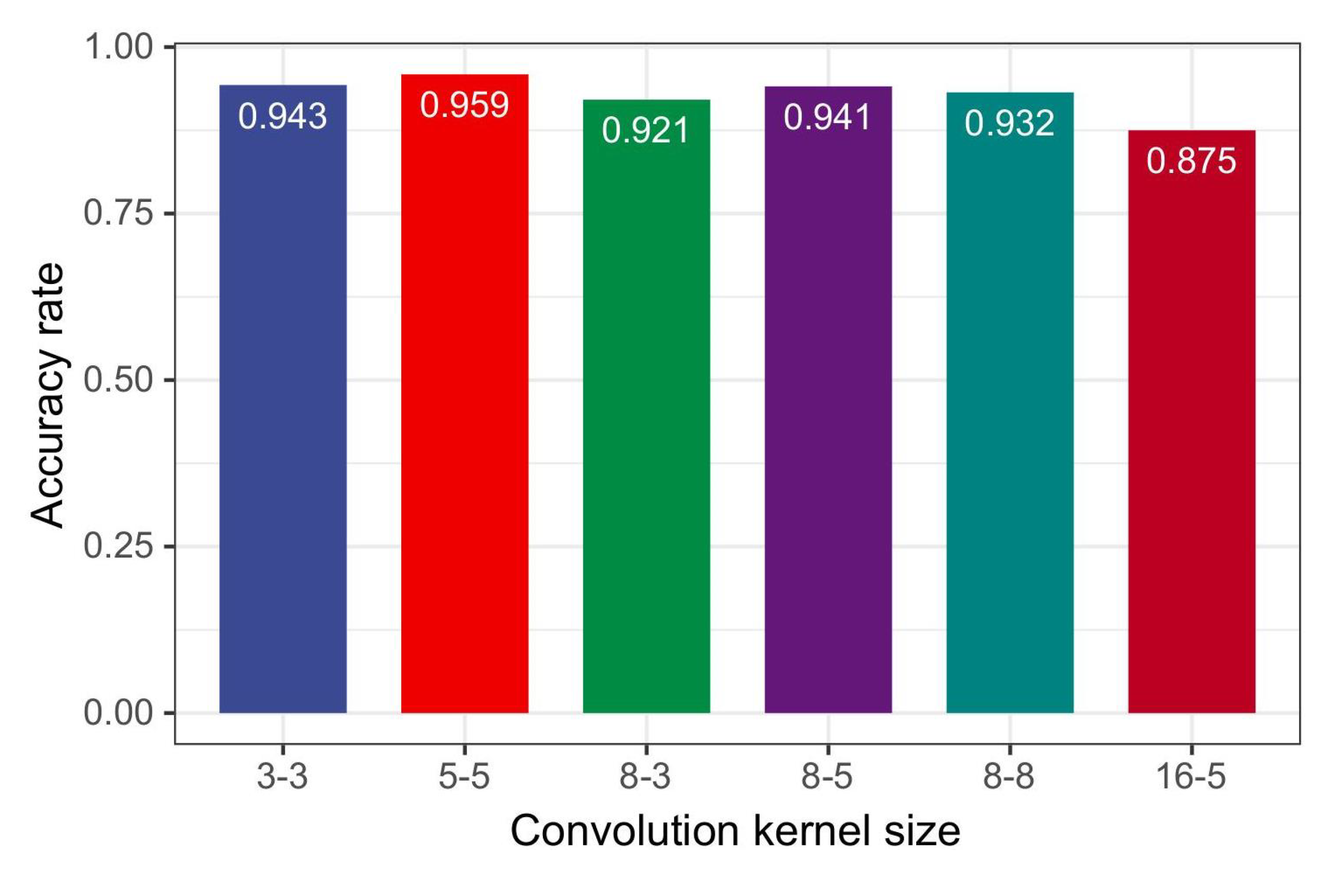
The size of kernels also has a great influence on the fault recognition ability of the fault diagnosis model. Dataset A is used for testing. As shown in Figure 7, convolution kernel size contains the size of the kernel of two convolution layers.
Figure 7 illustrates the shifting trend in model fault diagnosis accuracy, which first increases and then declines as kernel size grows. When the kernel size reaches 16, the model’s fault diagnosis accuracy decreases significantly. When the kernel size of two convolutional layers is set to 5-5, the correct rate of fault diagnosis is the highest. Therefore, the parameters of the proposed model are shown in Table 1.

4.2.2. Verification of Model Results

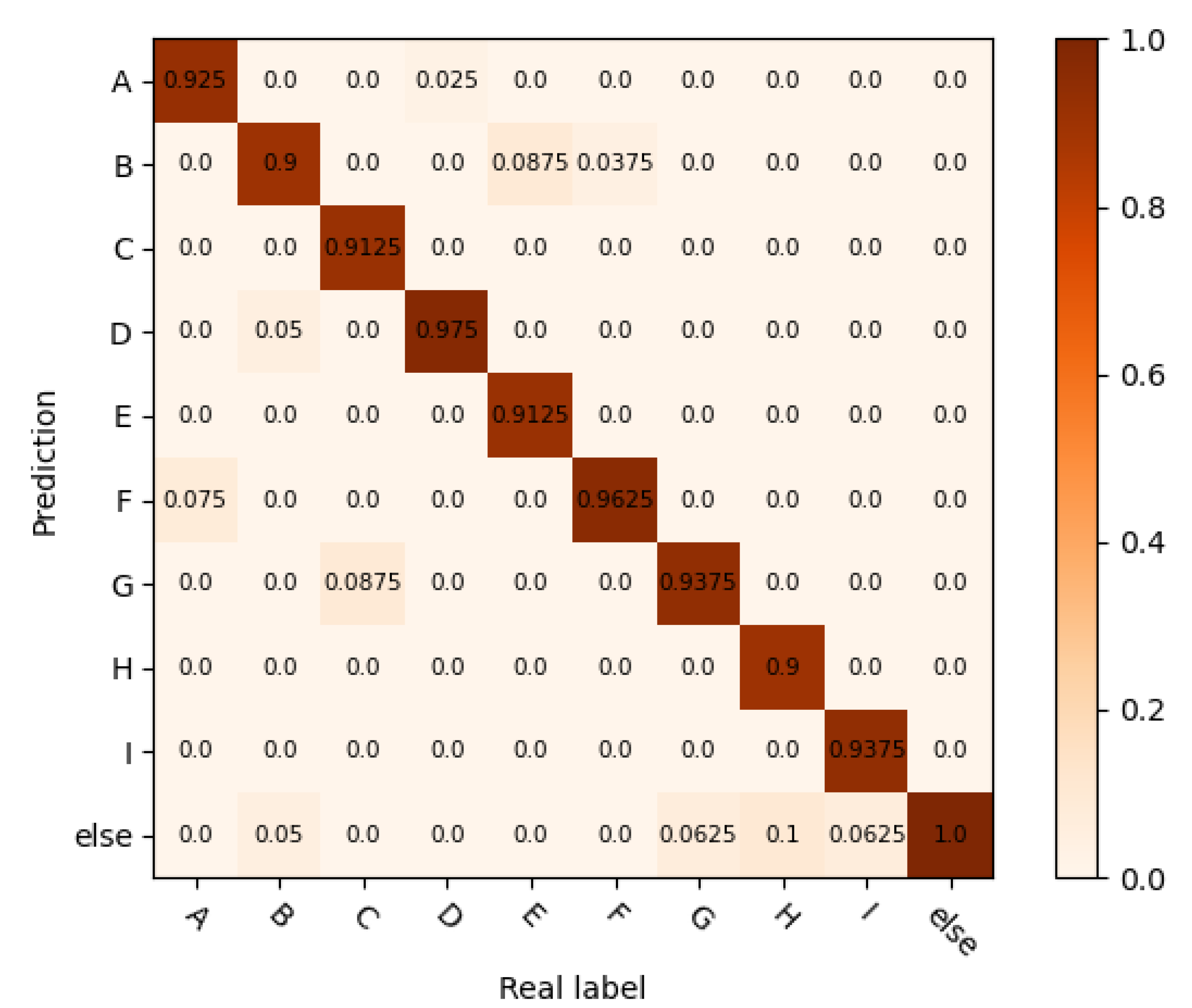
Figure 8 shows the confusion matrix of this model, which uses the data of the test set to test the model and selects nine faults from twenty-three kinds of faults for display. The classification of each fault type by the fault diagnosis model is displayed using the confusion matrix. It can be seen from Figure 8 that the failure type shown in Figure 8 is above 0.9, and the accuracy rate of most fault types is 1. Therefore, it can be proved that the model has excellent precision for all fault types.
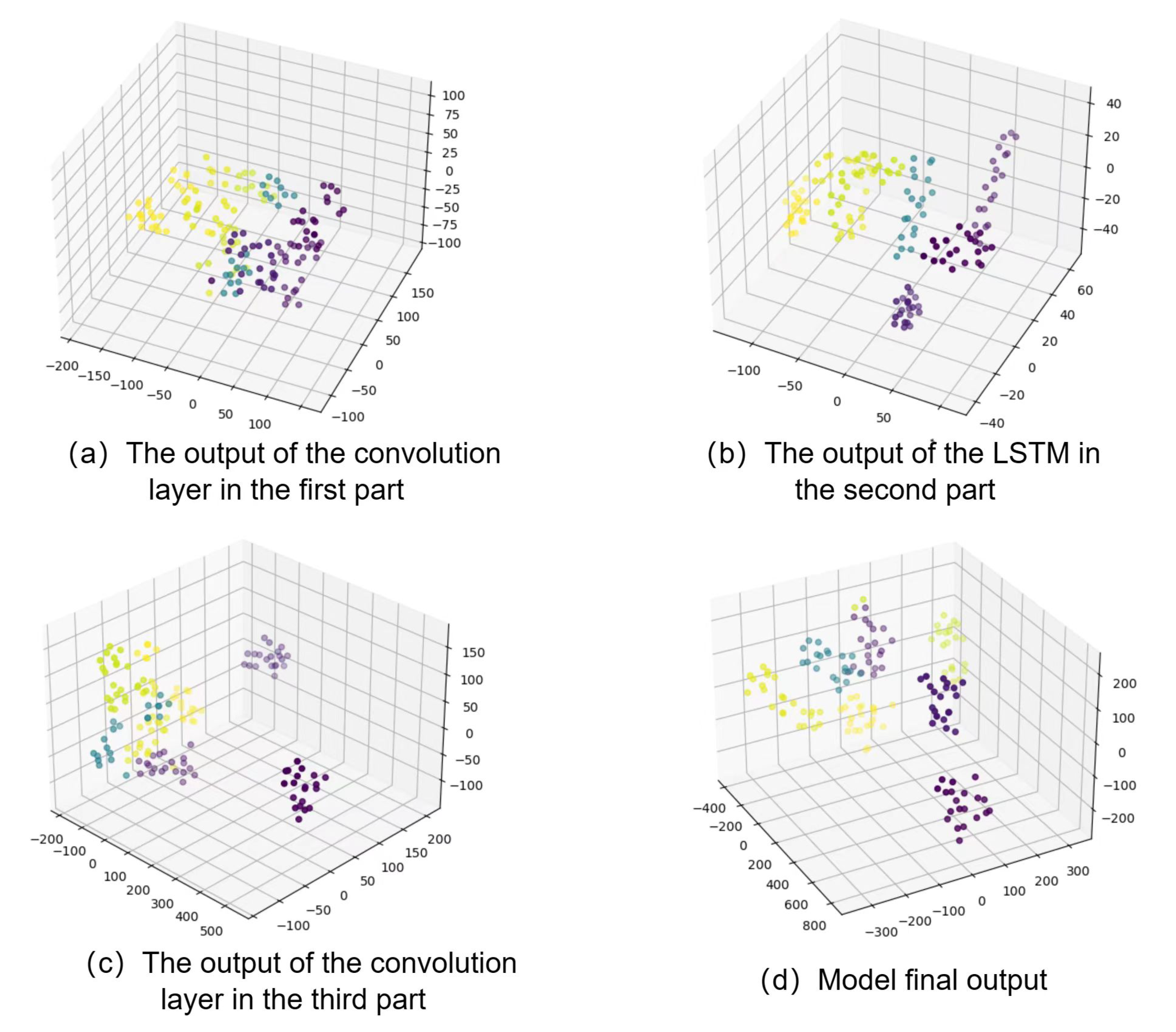
As shown in Figure 9, t-SNE is used to visualize the output of the four parts of the fault diagnosis model, and seven fault types are shown. Visualization of the classification process can clearly discover the classification of data by different structural layers so as to facilitate the study of the model. As seen from Figure 9, data of different fault types are relatively mixed after the convolution layer of the first part of the model. After the spatial–temporal characteristics of the data are extracted through the second part of the LSTM and the third part of the convolution layer, data of the same fault type are relatively aggregated, and fault data of different fault types begin to disperse. The proposed model’s output shows that the model has a decent classification effect for different fault types.

4.2.3. Model Comparison

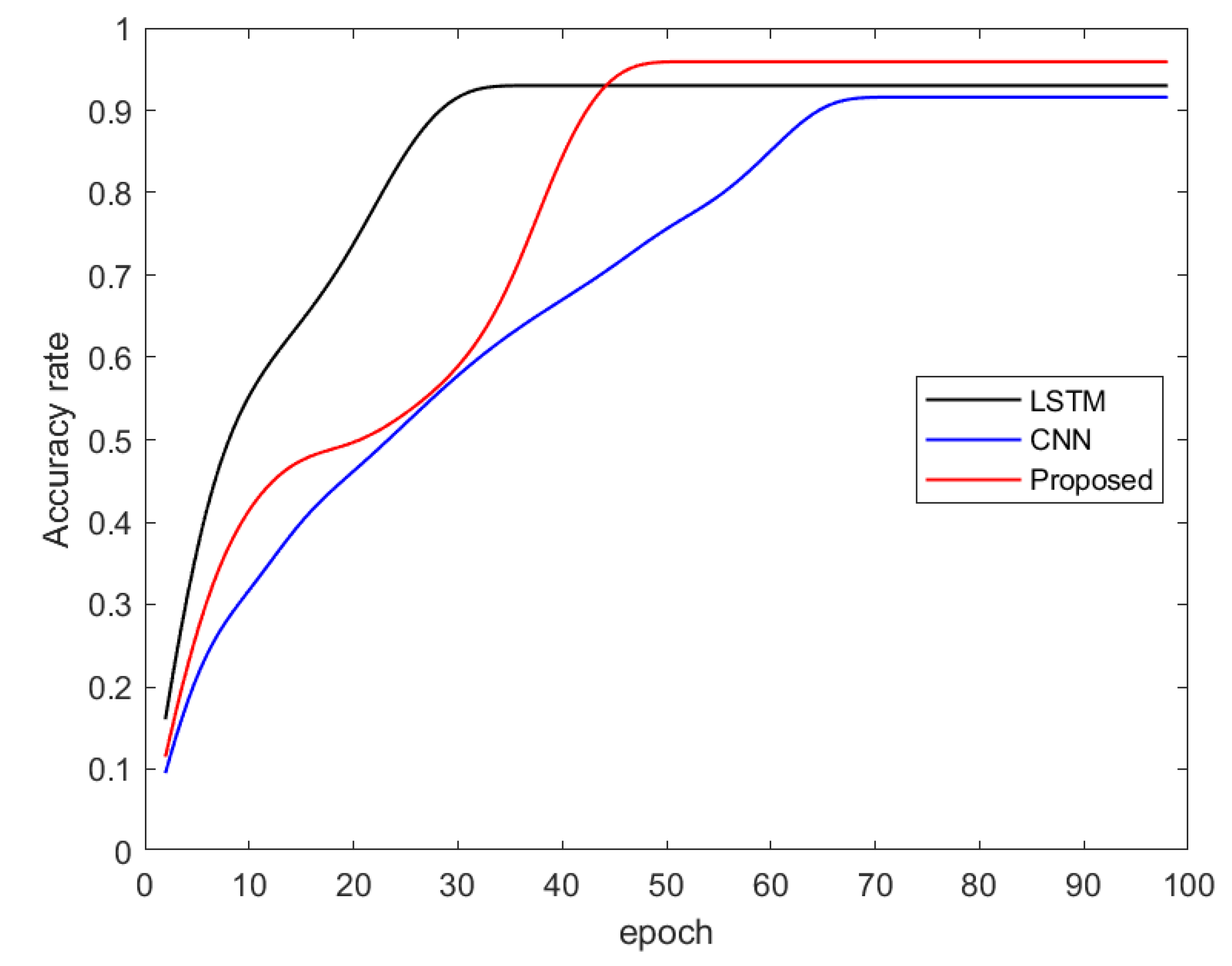
In order to verify the advantages of the proposed fault diagnosis model of dedicated equipment, the three models are trained several times. As shown in Figure 10, the changing trend of fault diagnosis accuracy rate of the models against the test set data during the training is compared. The CNN structure is the structure of the proposed model without LSTM, wherein the number of kernels of the two convolutional layers is 32. The structure of the LSTM model is the first and fourth part of the proposed model. As can be seen from Figure 10, compared with traditional CNN, adding LSTM can improve the feature extraction ability of the model for dedicated equipment data. For the LSTM model with single-layer LSTM, its fault diagnosis accuracy is not much improved compared with CNN, but it dramatically reduces the training time of the model. Although the training time of the proposed model is slightly longer than that of the LSTM model, the fault diagnosis accuracy has been significantly increased. Therefore, it is demonstrable that the proposed model has an excellent effect on the diagnosis of dedicated equipment faults.
Traditional fault diagnosis methods such as SVM were used in the past dedicated equipment, such as fire control system in dedicated equipment [34,35,36]. Due to data and other reasons, they did not obtain high accuracy of fault diagnosis, or they are not suitable for fault diagnosis research with large amounts of data. Since this paper uses hardware-on-loop simulation platform data for research, this paper uses neural network models that are excellent in other fields for comparative research. Table 4 shows the accuracy rates of different fault diagnosis models in dedicated equipment fault diagnosis. Model 1 is the proposed fault diagnosis model, model 2 is the model introduced above, and model 3 is a fault diagnosis model composed of two continuous layers of LSTM and two continuous layers of CNN [37]; this model uses two successive layers of LSTM to extract features from the data. Model 4 is a fault diagnosis model based on CNN [38]; this model is normalized by GN. Model 5 is the residual neural network model proposed in [1]; this model uses two residual blocks for feature extraction. Model 6 uses WDCNN for fault classification [39]; WDCNN uses wide convolution kernel to improve the classification of faults. As seen from Table 4, model 5 has the worst performance in fault identification. The fault diagnosis accuracy of model 6 is also slightly lower. The accuracy of models 2, 3, and 4 is not much different, but the accuracy of models 2 and 3 is higher than that of the CNN model. The results show that the proposed model has a better effect compared with other models.
Figure 11 shows the output classification of the four models after t-SNE dimension reduction. By reducing the dimensions of the output of different models, we can clearly find the fault classification degree of different models so as to facilitate the further study of the models.
Figure 11 shows seven fault types selected from twenty-three faults with a 100% accuracy rate. Data from dataset C are also used to detect the trained model, and each color represents a fault type. In Figure 11, (a) shows the output of model 4 in Table 4, (b) shows the output of model 2 in Table 4, (c) shows the output of the proposed model, and (d) shows the output of model 3 in Table 4. As observed from Figure 11, the output results of multiple fault types in (a) are relatively mixed, and the boundaries between different fault types are not obvious. The fault diagnosis model represented by (b) and (d) has a better classification effect on some fault types among the seven selected fault types than (a), but there are still some fault types with unclear classification boundaries. In contrast, the output results of different fault types in (c) are clearly distinguished. Therefore, it can be concluded that the proposed model based on CNN-LSTM has an excellent effect on the fault diagnosis of dedicated equipment.

5. Conclusions

Dedicated equipment is an essential part of ensuring the combat ability of a vehicle, and it is one of the most complex structures in the vehicle, so it is crucial to study the fault diagnosis of the dedicated equipment. This paper proposes a fault diagnosis algorithm based on CNN-LSTM to solve the problem of the fault diagnosis of dedicated equipment. In this model, LSTM is added to the traditional CNN so that the spatial–temporal features of the data can be extracted. Moreover, CBAM is incorporated into the model to enhance the capability of extracting critical features, hence enhancing fault diagnosis. The model is trained and tested with appropriate data obtained by a hardware-in-loop simulation platform. The model is then contrasted with other neural network models, and the findings demonstrate that the proposed algorithm has a strong capacity for dedicated equipment faults.
The dedicated equipment fault diagnosis model based on CNN-LSTM has good feature extraction and fault classification capabilities, which can provide potential solutions for the fault diagnosis problems of dedicated equipment. In the future, the fault diagnosis algorithm proposed in this paper will be validated using the data of actual vehicles.

Author Contributions

Methodology, Z.G., Y.H., Z.W. and Y.W.; Validation, Z.G., Y.H. and H.S.; Data curation, X.S.; Writing—original draft, Z.G. and Y.H.; Writing—review & editing, Y.W. All authors have read and agreed to the published version of the manuscript.

Funding

This research received no external funding.

Data Availability Statement

The data cannot be made public for secret restrictions.

Conflicts of Interest

The authors declare no conflict of interest.

References

  1. Zhang, W.; Li, X.; Ding, Q. Deep residual learning-based fault diagnosis method for rotating machinery. ISA Trans. 2019, 95, 295–305. [Google Scholar] [CrossRef] [PubMed]
  2. Wu, Y.; Hu, K.; Sun, X.; Ma, Y. Nonlinear Control of Quadrotor for Fault Tolerance: A Total Failure of One Actuator. IEEE Trans. Syst. Man Cybern. Syst. 2019, 51, 2810–2820. [Google Scholar] [CrossRef]
  3. Jia, F.; Lei, Y.; Guo, L.; Lin, J.; Xing, S. A neural network constructed by deep learning technique and its application to intelligent fault diagnosis of machines. Neurocomputing 2018, 272, 619–628. [Google Scholar] [CrossRef]
  4. Wang, Y.; Li, C.; Feng, J. Distributed pinning controllers design for set stabilization of k-valued logical control networks. Math. Model. Control 2023, 3, 61–72. [Google Scholar] [CrossRef]
  5. Young, C.C.; Yang, H.K. Fault detection in a ball bearing system using minimum variance spectrum. Meas. Sci. Technol. 2007, 18, 1433–1440. [Google Scholar]
  6. Yang, Y.; Yu, D.; Cheng, J. A fault diagnosis approach for roller bearing based on IMF envelope spectrum and SVM. Measurement 2007, 40, 943–950. [Google Scholar] [CrossRef]
  7. Klausen, A.; Robbersmyr, K.G.; Karimi, H.R. Autonomous Bearing Fault Diagnosis Method based on Envelope Spectrum. IFAC-PapersOnLine 2017, 40, 13378–13383. [Google Scholar] [CrossRef]
  8. Li, Y.; Wang, A.; Yi, X. Fire control system operation status assessment based on information fusion: Case study. Sensors 2019, 19, 2222. [Google Scholar] [CrossRef] [Green Version]
  9. Tan, C.; Yang, L.; Chen, H.; Xin, L. Fault diagnosis method for rolling bearing based on VMD and improved SVM optimized by METLBO. J. Mech. Sci. Technol. 2022, 36, 4979–4991. [Google Scholar] [CrossRef]
  10. Li, Y.; Song, L.; Sun, Q.; Xu, H.; Li, X.; Fang, Z.; Yao, W. Rolling bearing fault diagnosis based on quantum LS-SVM. EPJ Quantum Technol. 2022, 9, 1–15. [Google Scholar] [CrossRef]
  11. Mansouri, M.; Dhibi, K.; Nounou, H.; Nounou, M. Interval-Valued SVM Based ABO for Fault Detection and Diagnosis of Wind Energy Conversion Systems. IEEE Access 2022, 10, 130406–130414. [Google Scholar] [CrossRef]
  12. Cheng, J.; Feng, Z.; Xiong, Y. Transformer Fault Diagnosis Based on an Improved Sine Cosine Algorithm and BP Neural Network. Recent Adv. Electr. Electron. Eng. 2022, 15, 502–510. [Google Scholar]
  13. Hu, M.; Wu, J.; Yang, J.; Zhang, L.; Yang, F. Fault diagnosis of robot joint based on BP neural network. Robotica 2022, 40, 4388–4404. [Google Scholar] [CrossRef]
  14. Li, Z.; Zhang, Y.; Abu-Siada, A.; Chen, X.; Li, Z.; Xu, Y.; Zhang, L.; Tong, Y. Fault diagnosis of transformer windings based on decision tree and fully connected neural network. Energies 2021, 14, 1531. [Google Scholar] [CrossRef]
  15. Heaton, J.B.; Polson, N.G.; Witte, J.H. Deep learning for finance: Deep portfolios. Appl. Stoch. Model. Bus. Ind. 2017, 33, 3–12. [Google Scholar] [CrossRef]
  16. Shafay, M.; Ahmad, R.W.; Salah, K.; Yaqoob, I.; Jayaraman, R.; Omar, M. Blockchain for deep learning: Review and open challenges. Clust. Comput. 2023, 26, 197–221. [Google Scholar] [CrossRef]
  17. Alabdulkreem, E.; Alotaibi, S.S.; Alamgeer, M.; Marzouk, R.; Hilal, A.M.; Motwakel, A.; Zamani, A.S.; Rizwanullah, M. Intelligent Cybersecurity Classification Using Chaos Game Optimization with Deep Learning Model. Comput. Syst. Sci. Eng. 2023, 45, 971–983. [Google Scholar] [CrossRef]
  18. Niu, G.; Wang, X.; Golda, M.; Mastro, S.; Zhang, B. An optimized adaptive PReLU-DBN for rolling element bearing fault diagnosis. Neurocomputing 2021, 445, 26–34. [Google Scholar] [CrossRef]
  19. Gao, S.; Xu, L.; Zhang, Y.; Pei, Z. Rolling bearing fault diagnosis based on SSA optimized self-adaptive DBN. ISA Trans. 2022, 128, 485–502. [Google Scholar] [CrossRef]
  20. Van Tung, T.; AlThobiani, F.; Ball, A. An approach to fault diagnosis of reciprocating compressor valves using Teager-Kaiser energy operator and deep belief networks. Expert Syst. Appl. 2014, 41, 4113–4122. [Google Scholar] [CrossRef]
  21. Zhou, F.; Yang, S.; Fujita, H.; Chen, D.; Wen, C. Deep learning fault diagnosis method based on global optimization GAN for unbalanced data. Knowl.-Based Syst. 2020, 187, 104837. [Google Scholar] [CrossRef]
  22. Pham, M.T.; Kim, J.; Kim, C.H. Rolling Bearing Fault Diagnosis Based on Improved GAN and 2-D Representation of Acoustic Emission Signals. IEEE Access 2022, 10, 78056–78069. [Google Scholar] [CrossRef]
  23. Han, S.; Zhang, S.; Li, Y.; Chen, L. The multilabel fault diagnosis model of bearing based on integrated convolutional neural network and gated recurrent unit. Int. J. Intell. Comput. Cybern. 2022, 15, 401–413. [Google Scholar] [CrossRef]
  24. Zhang, Y.; Zhou, T.; Huang, X.; Cao, L.; Zhou, Q. Fault diagnosis of rotating machinery based on recurrent neural networks. Measurement 2021, 171, 108774. [Google Scholar] [CrossRef]
  25. Jalayer, M.; Orsenigo, C.; Vercellis, C. Fault detection and diagnosis for rotating machinery: A model based on convolutional LSTM, Fast Fourier and continuous wavelet transforms. Comput. Ind. 2021, 125, 103378. [Google Scholar] [CrossRef]
  26. Lei, J.; Liu, C.; Jiang, D. Fault diagnosis of wind turbine based on Long Short-term memory networks. Renew. Energy 2019, 133, 422–432. [Google Scholar] [CrossRef]
  27. Xiang, L.; Wang, P.; Yang, X.; Hu, A.; Su, H. Fault detection of wind turbine based on SCADA data analysis using CNN and LSTM with attention mechanism. Measurement 2021, 175, 109094. [Google Scholar] [CrossRef]
  28. Agarwal, P.; Gonzalez, J.I.M.; Elkamel, A.; Budman, H. Hierarchical Deep LSTM for Fault Detection and Diagnosis for a Chemical Process. Processes 2022, 10, 2557. [Google Scholar] [CrossRef]
  29. LeCun, Y.; Boser, B.; Denker, J.S.; Henderson, D.; Howard, R.E.; Hubbard, W.; Jackel, L.D. Backpropagation Applied to Handwritten Zip Code Recognition. Neural Comput. 1989, 1, 541–551. [Google Scholar] [CrossRef]
  30. Sinitsin, V.; Ibryaeva, O.; Sakovskaya, V.; Eremeeva, V. Intelligent bearing fault diagnosis method combining mixed input and hybrid CNN-MLP model. Mech. Syst. Signal Process. 2022, 180, 109454. [Google Scholar] [CrossRef]
  31. Janssens, O.; Slavkovikj, V.; Vervisch, B.; Stockman, K.; Loccufier, M.; Verstockt, S.; Van de Walle, R.; Van Hoecke, S. Convolutional Neural Network Based Fault Detection for Rotating Machinery. J. Sound Vib. 2016, 377, 331–345. [Google Scholar] [CrossRef]
  32. Yan, X.; Zhang, Y.; Jin, Q. Chemical Process Fault Diagnosis Based on Improved ResNet Fusing CBAM and SPP. IEEE Access 2023, 11, 46678–46690. [Google Scholar] [CrossRef]
  33. Zhang, L.; Duan, L. Cross-scenario transfer diagnosis of reciprocating compressor based on CBAM and ResNet. J. Intell. Fuzzy Syst. 2022, 43, 5929–5943. [Google Scholar] [CrossRef]
  34. Zhang, P.J.; Bo, Y.C.; Wang, H.Y.; Li, Q. Fault Diagnosis System of the Fire Control System Based on Fuzzy Neural Network. Adv. Mater. Res. 2013, 605, 828–831. [Google Scholar] [CrossRef]
  35. Zhang, C.; Feng, Q.; Bai, Z. Probabilistic Neural Network Application in Fault Diagnosis of Airborne Fire Control System. In Proceedings of the First Symposium on Aviation Maintenance and Management-Volume I; Springer: Berlin/Heidelberg, Germany, 2014; pp. 235–242. [Google Scholar]
  36. Li, Y.; Hu, X.; Yao, Z.; Zhang, Y. Fault diagnosis of fire control system based on genetic algorithm optimized BP neural network. In Proceedings of the 2022 Prognostics and Health Management Conference, London, UK, 27–29 May 2022; pp. 11–16. [Google Scholar]
  37. Mo, Y.; Xia, K.; Wang, H.; Su, H. Diagnosis Method Based on LSTM-CNN for Arc Fault in Brush and Slip Ring of Doubly-fed Induction Generator. Control Eng. China 2022, 29, 1520–1527. [Google Scholar]
  38. Chen, Z.; Mauricio, A.; Li, W.; Gryllias, K. A deep learning method for bearing fault diagnosis based on cyclic spectral coherence and convolutional neural networks. Mech. Syst. Signal Process. 2020, 140, 106683. [Google Scholar] [CrossRef]
  39. Zhang, W.; Peng, G.; Li, C.; Chen, Y.; Zhang, Z. A new deep learning model for fault diagnosis with good anti-noise and domain adaptation ability on raw vibration signals. Sensors 2017, 17, 425. [Google Scholar] [CrossRef] [Green Version]
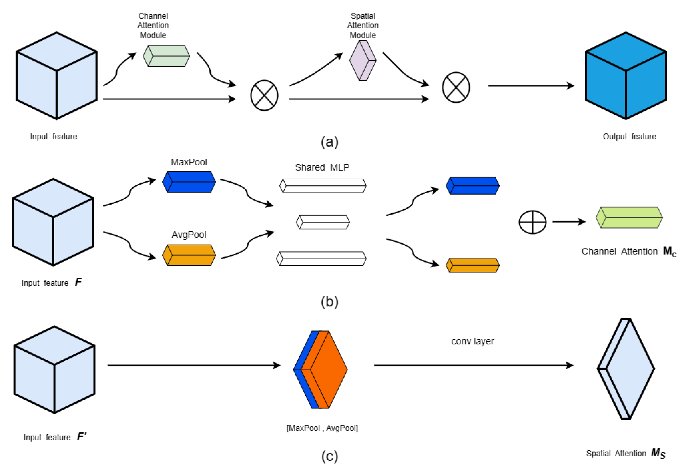
Figure 1. (a) Architecture of the CBAM (b) Architecture of the CAM (c) Architecture of the SAM.
Energies 16 05230 g001
Figure 2. Architecture of the LSTM.
Energies 16 05230 g002
Figure 3. Fault diagnosis model structure for dedicated equipment.
Energies 16 05230 g003
Figure 4. Fault diagnosis training methods for dedicated equipment.
Energies 16 05230 g004
Figure 5. Physical diagram of hardware-in-loop simulation platform.
Energies 16 05230 g005
Figure 6. (ac) Signal changes in 3 channels of dedicated equipment.
Energies 16 05230 g006
Figure 7. The recognition accuracy of fault diagnosis models with different kernel size.
Energies 16 05230 g007
Figure 8. Confusion matrix for testing data.
Energies 16 05230 g008
Figure 9. Visualization of fault diagnosis model identification process.
Energies 16 05230 g009
Figure 10. The changing trend in fault diagnosis accuracy of different models in the test set.
Energies 16 05230 g010
Figure 11. t-SNE dimension reduction analysis of output results of fault diagnosis model of dedicated equipment.
Energies 16 05230 g011
Table 1. Parameters of the fault diagnosis model.
Network LayerKernel SizeNumber of KernelsStep Size
Cov581
Pool3 1
LSTM 16
Cov5161
Pool3 1
LSTM 8
Table 2. I/0 signals.
SignalSignal Value/V
123.4–28.6
221.4–30.6
323.4–28.6
421.4–30.6
521.4–30.6
621.4–30.6
7−4.5–5.5
823.4–28.6
Table 3. The recognition accuracy of the proposed models with the different number of kernels.
Number of KernelsDataset ADataset BDataset C
8-10-891.15%90.89%90.7%
8-10-1688.1%87.3%87.8%
8-16-894.37%93.98%94.52%
8-16-323%3%3%
8-32-163%3%3%
Table 4. Comparison of fault diagnosis accuracy of different models.
Model NumberModel NameAccuracy Rate
1Proposed95.9%
2LSTM93.0%
3LSTM-CNN92.2%
4CNN92.4%
5ResNet75.2%
6WDCNN90.1%
Disclaimer/Publisher’s Note: The statements, opinions and data contained in all publications are solely those of the individual author(s) and contributor(s) and not of MDPI and/or the editor(s). MDPI and/or the editor(s) disclaim responsibility for any injury to people or property resulting from any ideas, methods, instructions or products referred to in the content.