
A Practical Model for Gas–Water Two-Phase Flow and Fracture Parameter Estimation in Shale

Abstract
:1. Introduction
2. Mathematical Model for Gas-Water Two-Phase Flow
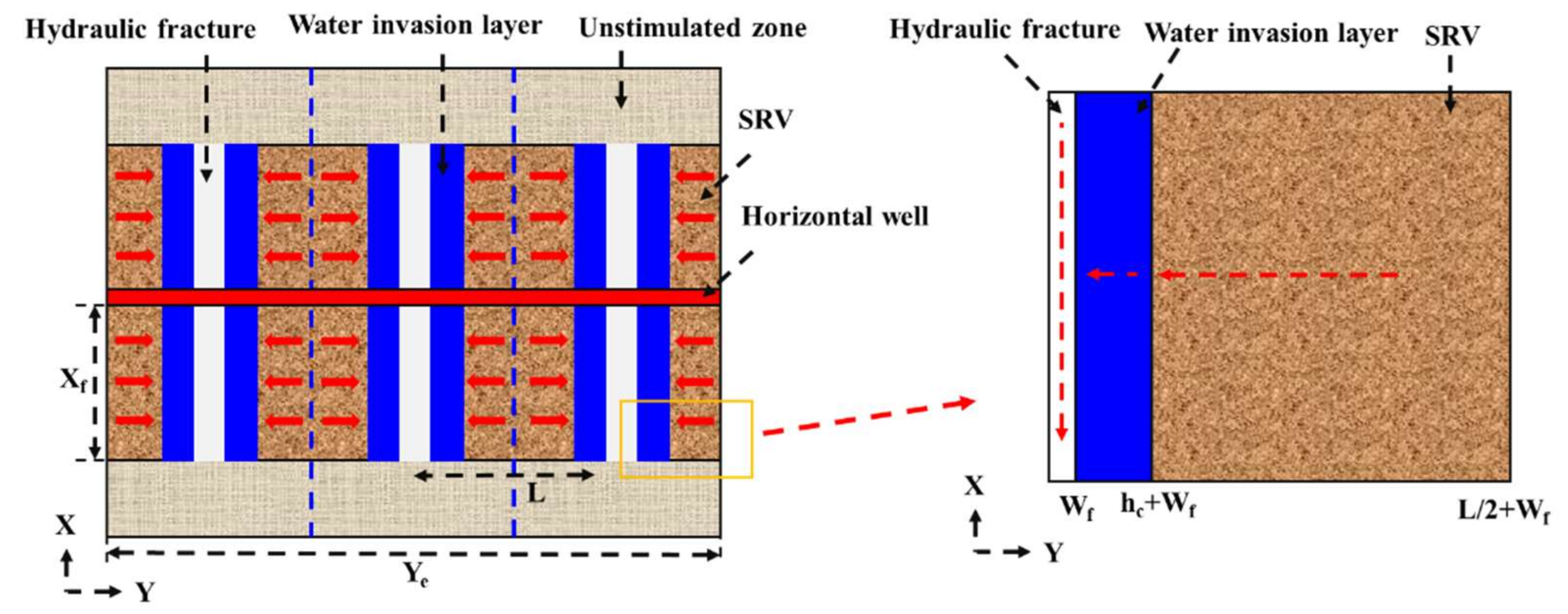
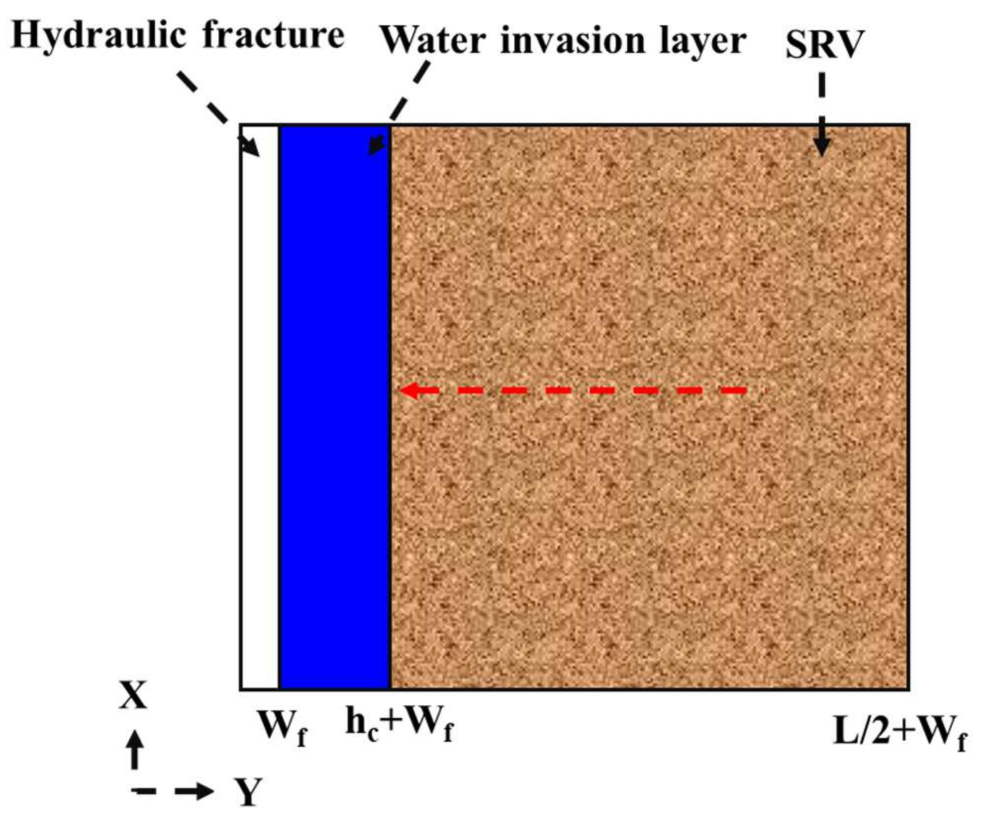
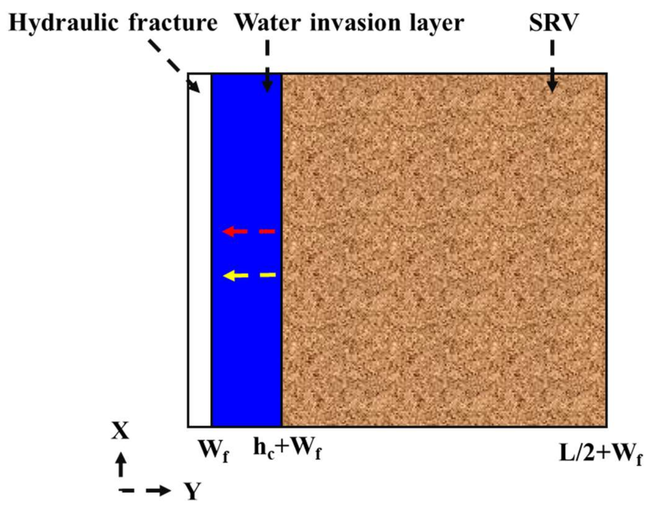
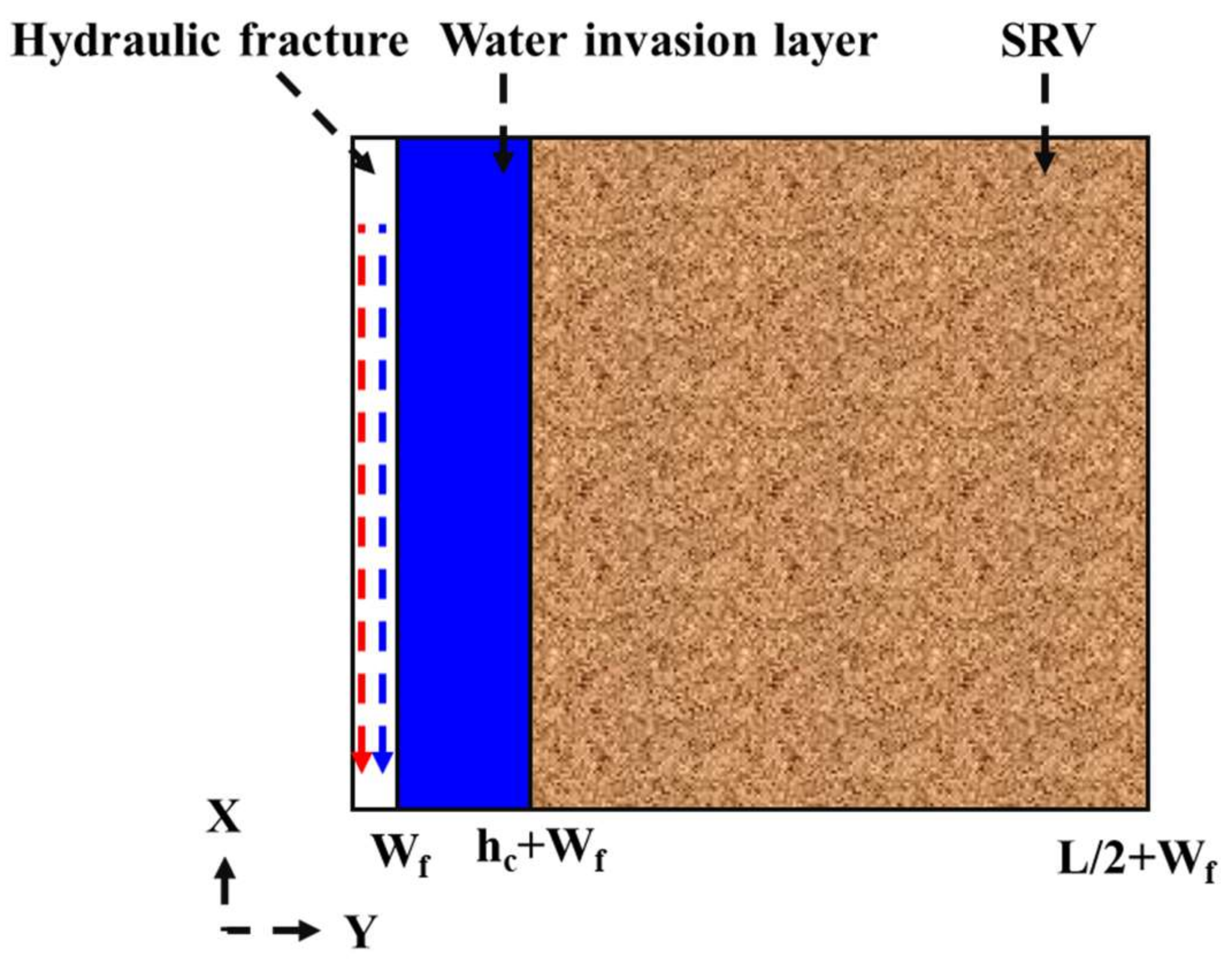
2.1. Physical Model and Assumptions
- (1)
- The reservoir is of equal thickness, homogeneous and closed. The horizontal well maintains constant pressure production.
- (2)
- Gas flow is considered to be single-phase in the SRV, and gas–water two-phase flow is considered in the water invasion layer and hydraulic fracture.
- (3)
- The effects of gas desorption and slippage are considered in the shale matrix, and the stress sensitivity of hydraulic fracture is considered.
2.2. Single-Phase Gas Flow in Stimulated Reservoir
2.3. Gas-Water Two-Phase Flow in Water Invasion Layer
2.4. Gas-Water Two-Phase Flow in Hydraulic Fracture
2.5. Dimensionless Model and Lapalce Transform
3. Solution of Gas–Water Two-Phase Flow Model
3.1. Solution of Gas Flow Equation
3.2. Solution of Water Flow Equation
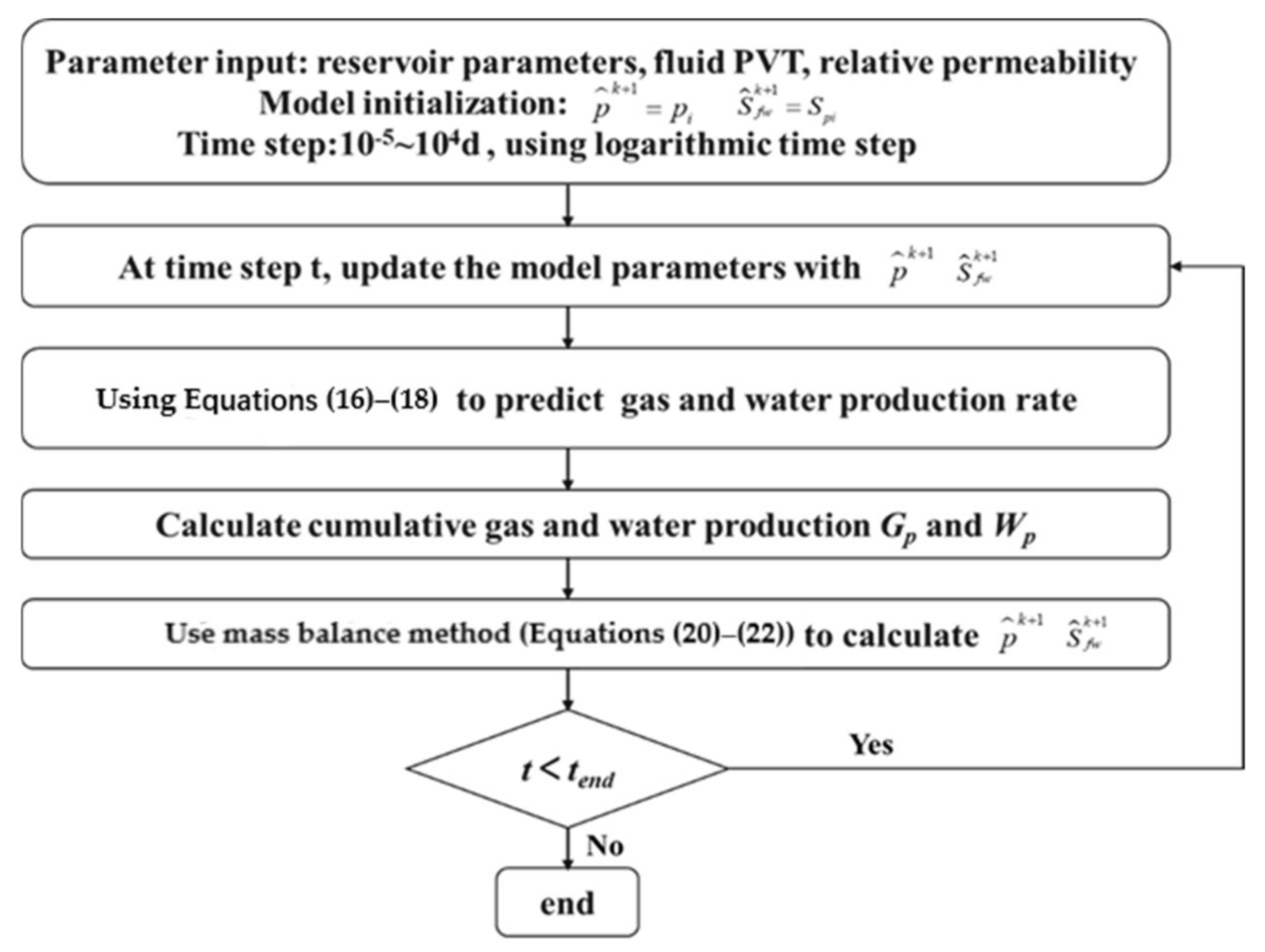
3.3. Solution Procedure of the Model
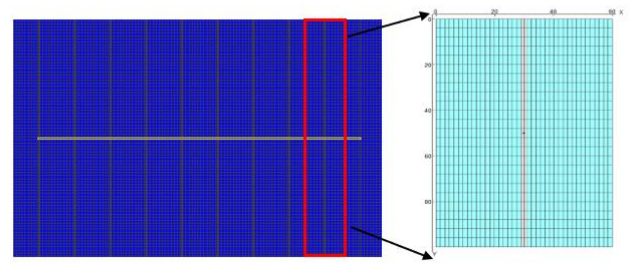
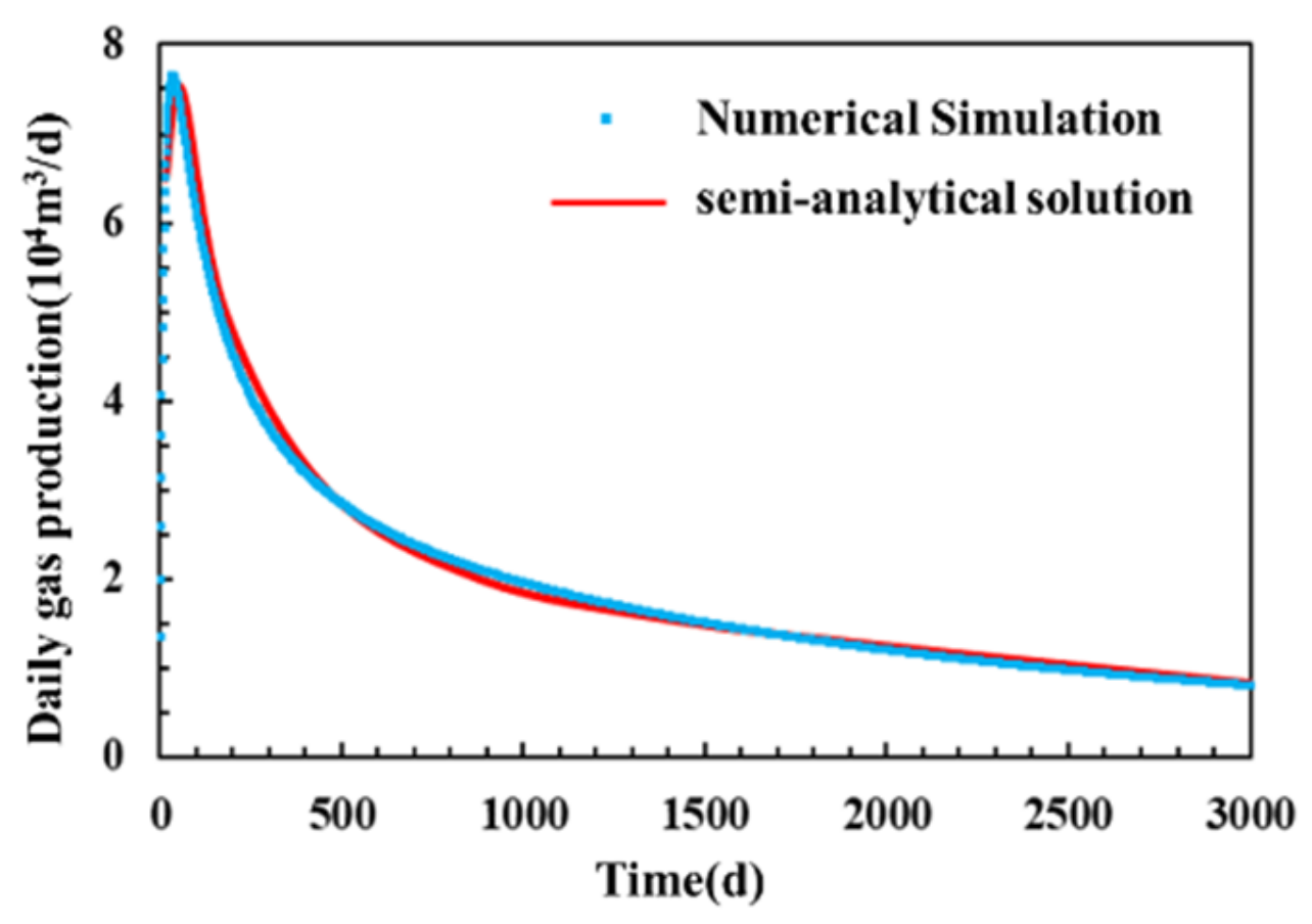
3.4. Model Validation
4. Interpretation of Fracture Network Parameters
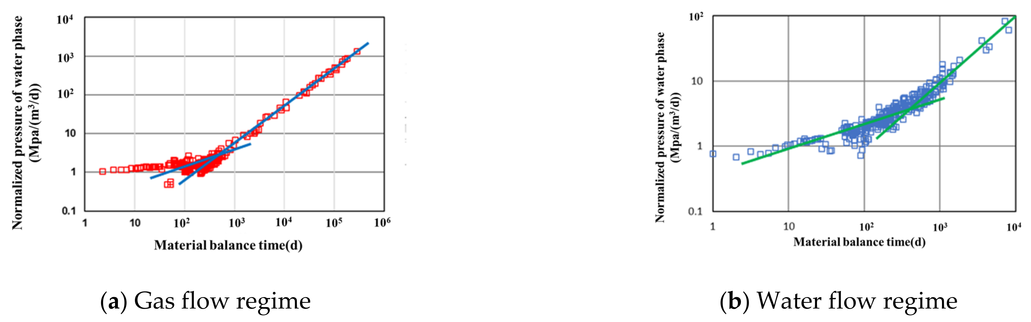
4.1. Flow Regimes of Gas-Water
4.1.1. Flow Regimes of Gas-Water in the First Mode
- (1)
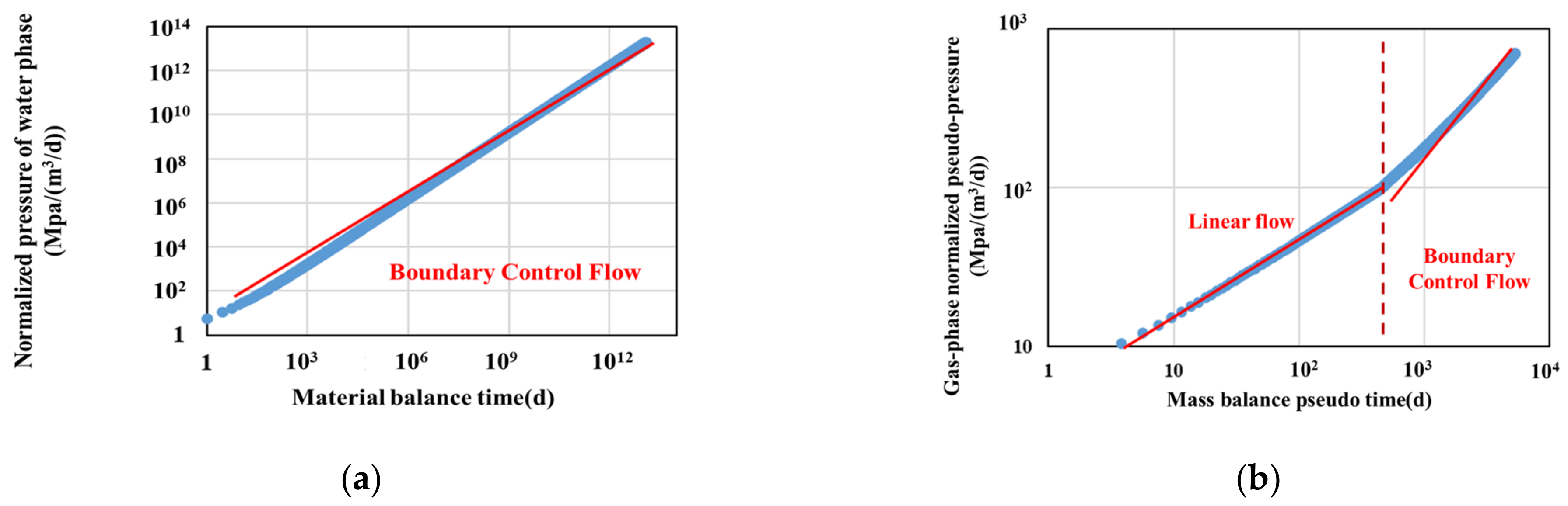
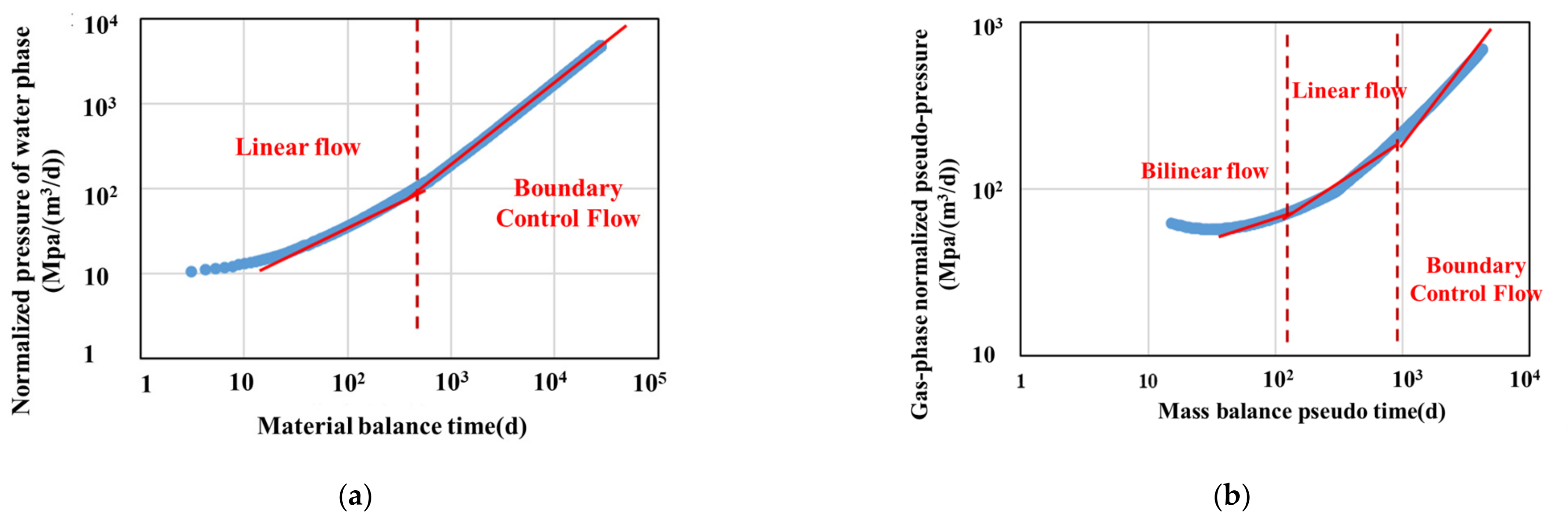
- Water boundary dominated flow. Because the fracturing fluid mainly occurs in the hydraulic fracture, water will drain very fast and then show the boundary dominated flow, until the water production rate is nearly zero. On the plot of rate normalized pressure and mass balance time, the curve shows a unit slope straight line.
- (2)
- Gas linear flow. This flow regime occurs at almost the same time with a water boundary dominated flow, and is the first flow stage of the gas phase. At this time, the gas in the matrix flows to the fracture in a direction perpendicular to the fracture surface, which appears as straight with one-half slope on the typical curve.
- (3)
- Gas boundary dominated flow. With the production, the gas pressure drop reaches the closed boundary and forms the boundary dominated flow, which is represented as a straight line with a unit slope on the typical curve shown.
4.1.2. Flow Regimes of Gas-Water in the Second Mode
- (1)
- Water linear flow. Since fracturing fluid exists in both the hydraulic fracture and the invasion layer, linear flow of the water phase will occur when the pressure drop in the water invasion layer after the flowback starts. The typical curve shows a straight line with a unit slope.
- (2)
- Water boundary dominated flow. Due to the fracturing fluid mainly occurs in the hydraulic fracture, water will drain very fast and then show the boundary dominated flow, until the water production rate is nearly zero. On the plot of rate normalized pressure and mass balance time, the curve shows a unit slope straight line.
- (3)
- Gas bilinear flow. Gas phase flow into the hydraulic fracture soon after the flowback starts and forms bilinear flow with the pressure drop system formed by the water invasion layer and shale matrix, which is represented as a straight line with a quarter-slope.
- (4)
- Gas linear flow. This flow regime occurs at almost the same time with water boundary dominated flow, and is the first flow stage of the gas phase. At this time, the gas in the matrix flows to the fracture in a direction perpendicular to the fracture surface, which appears as a straight line with one-half slope on the typical curve.
- (5)
- Gas boundary dominated flow. With the production, the gas pressure drop reaches the closed boundary and forms the boundary dominated flow, which is represented as a straight line with a unit slope on the typical curve shown.
4.2. Interpretation Procedure Fracture Network Parameters
- (1)
- Initial parameter input: set the initial value of the parameters of fracture network, including the fracture half-length, the fracture permeability, the thickness of the water invasion layer, the permeability of the water invasion layer, the width and permeability of the SRV. Additionally, set .
- (2)
- Take days as the time step, and update the parameters of the gas–water flow model with the , .
- (3)
- Constant pressure solution: gas and water production are calculated by using the gas–water two-phase flow model.
- (4)
- Variable pressure solution: Equation (23) is used to obtain the gas production and water production under variable bottomhole flow pressure.
- (5)
- Calculation of average pressure and saturation: the average pressure and saturation calculated by the material balance method are then substituted into step (2) for recurrent calculation.
- (6)
- If the fitting error between simulated and actual data meets the criterion of convergence, the calculation is finished. Otherwise, update the fitting parameters and repeat the above steps.
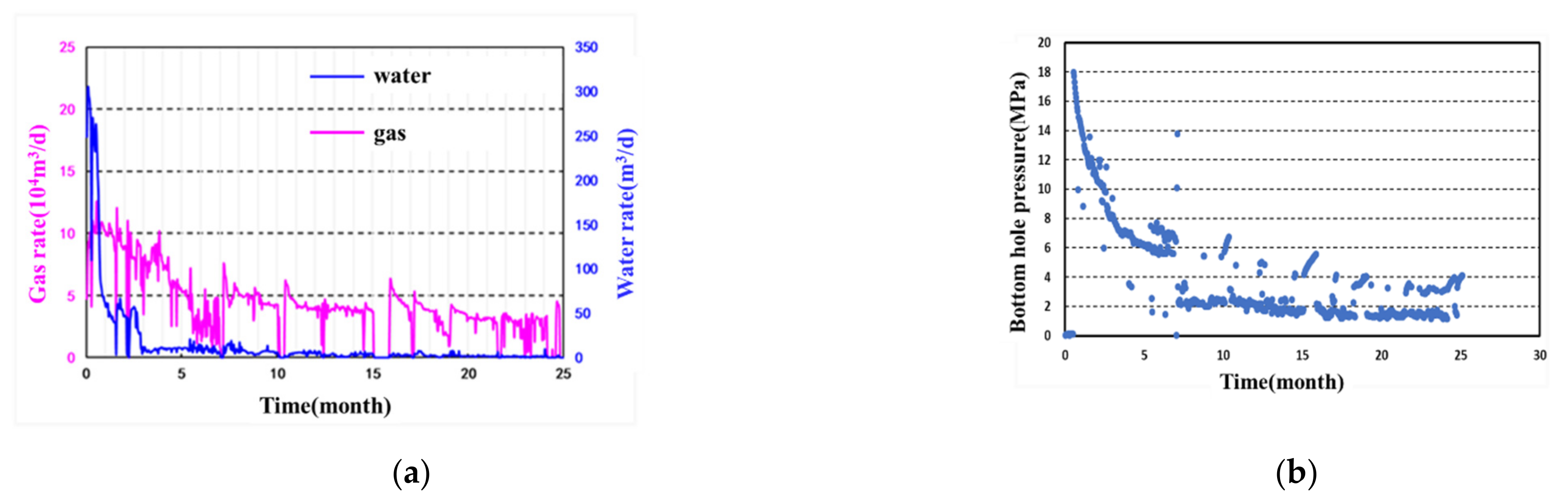
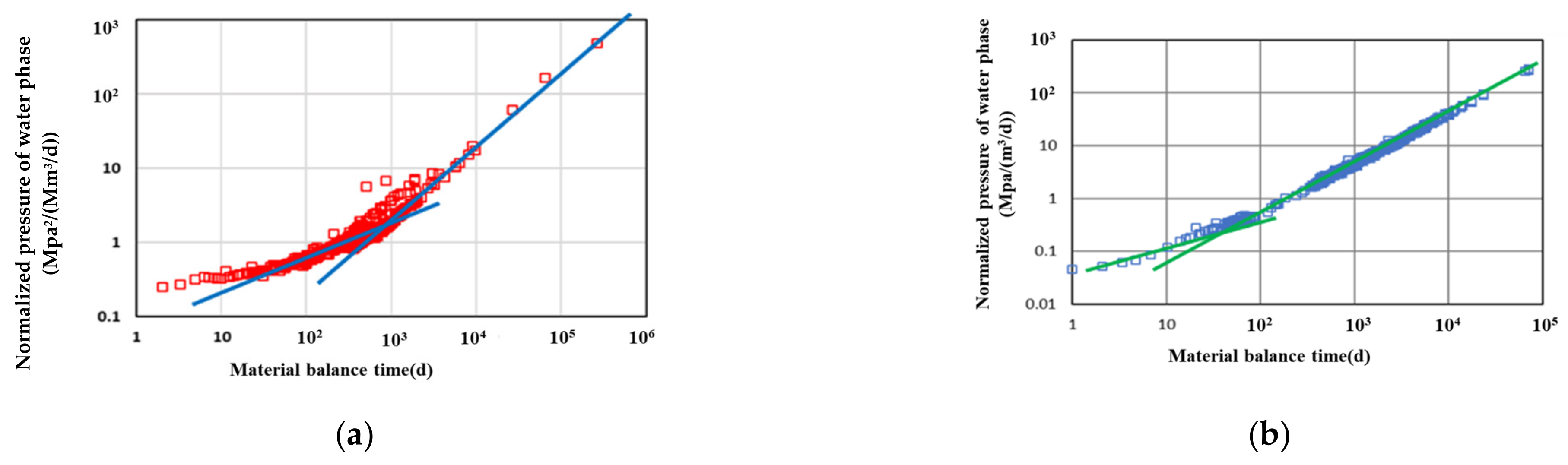
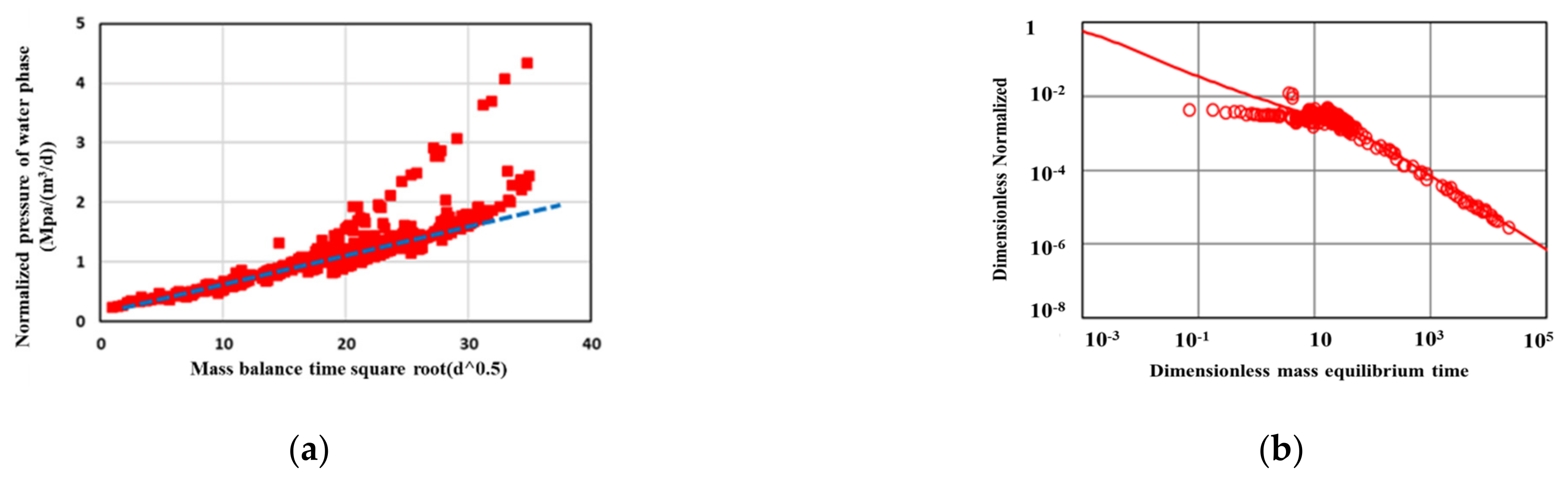
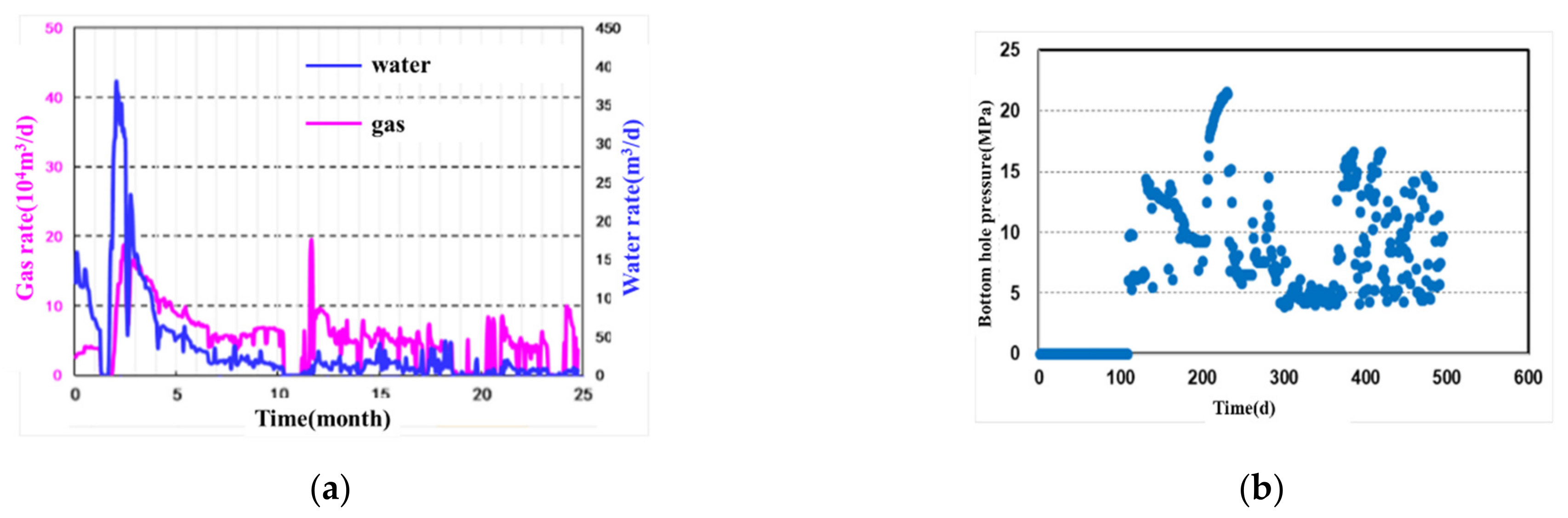
4.3. Field Exmaple
4.3.1. Well A
4.3.2. Well B
5. Conclusions
- In this paper, a practical model considering gas adsorption of the shale matrix, water invasion layer and gas–water two-phase flow of hydraulic fracture is established, and the semi-analytical solution method is developed.
- The new model is used to successfully analyze the production performance of the two modes of gas and water production. The two cases show different gas and water flow regimes:
- (1)
- The first production mode mainly shows three flow regimes, including water boundary dominated flow, gas linear flow and gas boundary dominated flow.
- (2)
- The second production mode mainly shows five flow stages, including water linear flow, water boundary dominated flow, gas bilinear flow, gas linear flow and gas boundary dominated flow.
- The developed fracture parameters interpretation method can reasonably estimate the key parameters of the hydraulic fracture, water invasion layer and SRV of fracture well from the field example.
Author Contributions
Funding
Data Availability Statement
Conflicts of Interest
Appendix A
Appendix B
Appendix C
References
- Wattenbarger, R.; El-Banbi, A.; Villegas, M.; Maggard, J.B. Production analysis of linear flow into fractured tight gas wells. In Proceedings of the SPE Rocky Mountain Regional/Low-Permeability Reservoirs Symposium, Denver, CO, USA, 5–8 April 1998. [Google Scholar]
- Bello, R.O.; Wattenbarger, R.A. Modelling and Analysis of Shale Gas Production with a Skin Effect. J. Can. Pet. Technol. 2010, 49, 37–48. [Google Scholar] [CrossRef]
- Alahmadi, H.A.H.; Wattenbarger, R.A. Triple-porosity models: One further step towards capturing fractured reservoirs heterogeneity. In Proceedings of the SPE/DGS Saudi Arabia Section Technical Symposium and Exhibition, Al-Khobar, Saudi Arabia, 15–18 May 2011. [Google Scholar]
- Brown, M.L.; Ozkan, E.; Raghavan, R.S.; Kazemi, H. Practical Solutions for Pressure-Transient Responses of Fractured Horizontal Wells in Unconventional Shale Reservoirs. SPE Reserv. Eval. Eng. 2009, 14, 663–676. [Google Scholar] [CrossRef]
- Stalgorova, K.; Mattar, L. Analytical Model for Unconventional Multifractured Composite Systems. SPE Reserv. Eval. Eng. 2013, 16, 246–256. [Google Scholar] [CrossRef]
- Shuang, A. Productivity Evaluation and Production Rule of Fractured Horizontal Wells in Shale Gas. Master’s Thesis, China University of Petroleum, Beijing, China, 2015. [Google Scholar]
- AlQuaimi, B.I.; Rossen, W.R. Capillary Desaturation Curve for Residual Nonwetting Phase in Natural Fractures. SPE J. 2018, 23, 788–802. [Google Scholar] [CrossRef]
- Chen, Y.; Fu, L.; Hao, M. Derivation and application of gas adsorption equation and desorption equation. China Offshore Oil Gas 2018, 30, 85–89. [Google Scholar]
- Stehfest, H. Numerical Estimation of Laplace Transforms. ACM Commun. 1970, 13, 47–49. [Google Scholar] [CrossRef]


| Dimensionless Parameters | Define |
|---|---|
| Dimensionless x | |
| Dimensionless time | |
| Dimensionless permeability | |
| Dimensionless y | |
| Dimensionless pseudo-time | |
| Dimensionless hydraulic fracture conductivity |
| Parameter | The Numerical |
|---|---|
| Fracture porosity, % | 45 |
| Crack compression coefficient, MPa−1 | 1.0 × 10⁻³ |
| Fracture permeability, mD | 1000 |
| Crack half-length, M | 100 |
| Initial fracture water saturation, % | 100 |
| Matrix compression coefficient, MPa−1 | 1.0 × 10⁻⁴ |
| Width of water invasion layer, m | 2 |
| Matrix permeability, mD | 1.0 × 10⁻⁴ |
| Effective reservoir thickness, m | 10 |
| Initial gas saturation of the matrix, % | 70 |
| Initial crack pressure, MPa | 29.5 |
| Matrix porosity, % | 6.4 |
| Bottom hole flow pressure, MPa | 2 |
| Permeability of water invasion layer, mD | 5.0 × 10⁻⁵ |
| Flow Regime | Description | Schematic Diagram |
|---|---|---|
| Water boundary dominated flow | The fracturing fluid flows along the hydraulic fracture into the wellbore, and the water exhibits depletion in the fracture | 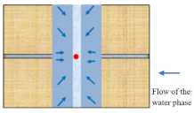 |
| Gas linear flow | Gas in matrix flows into the fracture in a direction perpendicular to the fracture surface, and the gas dominates the fracture flow |  |
| Gas boundary dominated flow | After the gas pressure drop boundary reaches the closed boundary, the closed boundary control flow is formed | 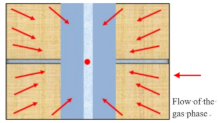 |
| Liquid Phase | Flow Phase Description | Schematic Diagram |
|---|---|---|
| Water linear flow | The water fluid flows linearly to the wellbore along the invasion layer. This stage occurs at the beginning of the flowback. | 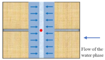 |
| Water boundary dominated flow | The fracturing fluid flows along the hydraulic fracture into the wellbore, and the water exhibits depletion in the fracture | 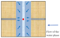 |
| Gas linear flow | Gas in matrix flows into the fracture in a direction perpendicular to the fracture surface, and the gas dominates the fracture flow | 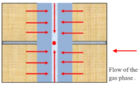 |
| Gas boundary dominated flow | After the gas pressure drop boundary reaches the closed boundary, the closed boundary control flow is formed | 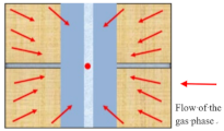 |
| Parameter | Value |
|---|---|
| Initial pressure, MPa | 29.65 |
| Initial gas saturation, decimal | 0.6 |
| Reservoir temperature, K | 358.1 |
| Reservoir thickness, m | 15 |
| Langmuir volume | 2.86 |
| Langmuir pressure, MPa | 9.18 |
| Horizontal well length, m | 1441 |
| Number of fractures | 25 |
| Matrix porosity | 0.064 |
| Matrix Compressibility, MPa−1 | 8 × 10⁻⁵ |
| Fracture Compressibility, MPa−1 | 8 × 10⁻⁵ |
| Fracture width, m | 0.5 × 10⁻² |
| Interpreted Parameters | Value |
|---|---|
| Fracture half-length (m) | 83.1 |
| Fracture permeability (mD) | 865 |
| Thickness of water invasion layer (m) | 0.12 |
| Permeability of water invasion (mD) | 2.82 × 10⁻³ |
| SRV width (m) | 46.5 |
| SRV Permeability (mD) | 3.87 × 10⁻³ |
| Parameter | Value |
|---|---|
| Initial pressure, MPa | 31.15 |
| Initial gas saturation, decimal | 0.6 |
| Reservoir temperature, K | 383.1 |
| Reservoir thickness, m | 10 |
| Langmuir volume | 1.96 |
| Langmuir pressure, MPa | 2200 |
| Horizontal well length, m | 1266 |
| Number of fractures | 19 |
| Matrix porosity | 0.064 |
| Matrix Compressibility, MPa−1 | 8 × 10⁻⁵ |
| Fracture Compressibility, MPa−1 | 8 × 10⁻⁵ |
| Fracture width, m | 0.5 × 10⁻² |
| Interpreted Parameters | Value |
|---|---|
| Fracture half-length (m) | 82.1 |
| Fracture permeability (mD) | 685 |
| Thickness of water invasion layer (m) | 0.91 |
| Permeability of water invasion (mD) | 1.95 × 10⁻³ |
| SRV width (m) | 45.3 |
| SRV Permeability (mD) | 3.12 × 10⁻³ |
Disclaimer/Publisher’s Note: The statements, opinions and data contained in all publications are solely those of the individual author(s) and contributor(s) and not of MDPI and/or the editor(s). MDPI and/or the editor(s) disclaim responsibility for any injury to people or property resulting from any ideas, methods, instructions or products referred to in the content. |
© 2023 by the authors. Licensee MDPI, Basel, Switzerland. This article is an open access article distributed under the terms and conditions of the Creative Commons Attribution (CC BY) license (https://creativecommons.org/licenses/by/4.0/).
Share and Cite
Jia, P.; Niu, L.; Li, Y.; Feng, H. A Practical Model for Gas–Water Two-Phase Flow and Fracture Parameter Estimation in Shale. Energies 2023, 16, 5140. https://doi.org/10.3390/en16135140
Jia P, Niu L, Li Y, Feng H. A Practical Model for Gas–Water Two-Phase Flow and Fracture Parameter Estimation in Shale. Energies. 2023; 16(13):5140. https://doi.org/10.3390/en16135140
Chicago/Turabian StyleJia, Pin, Langyu Niu, Yang Li, and Haoran Feng. 2023. "A Practical Model for Gas–Water Two-Phase Flow and Fracture Parameter Estimation in Shale" Energies 16, no. 13: 5140. https://doi.org/10.3390/en16135140
APA StyleJia, P., Niu, L., Li, Y., & Feng, H. (2023). A Practical Model for Gas–Water Two-Phase Flow and Fracture Parameter Estimation in Shale. Energies, 16(13), 5140. https://doi.org/10.3390/en16135140