Modernization Roadmaps for Existing Buildings under Limited Energy Resources and Craftwork Capacities

Abstract

Great potential for saving carbon emissions lies in modernizing European buildings. Multi-year modernization roadmaps can plan modernization measures in terms of time and are able to consider temporal interactions. Therefore, we have developed a mixed-integer program that determines modernization roadmaps. These roadmaps include changing the energy supply system, improving the envelope, and considering annually varying boundary conditions. High craftwork capacities are required to implement the necessary modernizations to meet climate goals. Unfortunately, studies showed that the current shortage of craftworkers will intensify in the next years. Other important limitations correspond to energy resources. Recent crises show that many energy systems need to handle these limitations. Therefore, we extended the mixed-integer program by a method to handle these limitations inside the roadmaps. By the use of data from 90 interviews with craftwork specialists about the time needed to realize modernization measures, the method is applied. The main purpose is to analyze how modernization strategies change under limited resources, especially in terms of craftwork capacities. Hence, the method is exemplified by a representative single-family dwelling. Within this use case, modernization roadmaps with different craftwork capacity levels were calculated. The results show that modernization roadmaps change comprehensively over these levels. Key findings are that costs and emissions rise with decreasing craftwork capacities. Furthermore, smaller storages and pv systems are implemented at low craftwork capacities. The electrification of the heat supply supported by medium insulation standards should also be implemented with limited craftwork capacities.

1. Introduction

Existing buildings contribute to climate change with 28% of the global carbon emissions [1]. More than 50% of the European buildings were built before 1980 without ambitious regularities on energy efficiency [2]. Since these buildings are responsible for more than 60% of the demand of all European buildings [2], a large emission-saving potential lies in modernizing them and the majority of the rest of the building stock.

Optimization models as rational decision makers are used widely in energy research to design building energy systems. In the last decades, many works of this field have contributed to the modernization of buildings [3].

Because of different lifetimes of devices and components in building energy systems, limited craftwork capacities and investment possibilities as well as further individual reasons, it should be considered that multiple points in time are necessary to modernize a building.

Costa-Carrapiço et al. [4] analyzed over 500 studies and found that the long-term behavior of buildings in a changing environment, such as climate change, is rarely studied. Furthermore, the studies are used to determine building designs for one point in time and do not include temporal planning [4]. In their review, Fodstad et al. [5] stated that the temporal dimension in energy system modeling is important and should be considered in more depth at different levels of modeling.

In the realm of building modernization research, the aspect of long-term temporal planning remains relatively unexplored. Thus far, the prevalent approaches focus on single-year optimization methods, wherein decisions are exclusively made at the onset of the designated observation period (e.g., [6,7,8]). Conversely, endeavors that incorporate temporal considerations in building modernization predominantly revolve around the prioritization of modernization sequences within building portfolios (e.g., [9]) or the analysis of future boundary conditions through scenario assessments, such as evolving climate conditions (e.g., [10]).

In contrast, multi-year approaches consider more than one point in time for the decisions. These approaches have already been used in other fields of energy research, such as designing microgrids [11] and distributed energy systems [12], and were proven to lead to better ecological and economic performances than single-year approaches [13,14]. Advantages are the possibility of using time-varying parameters such as energy prices and design decisions at different points in time that can be modeled dependent on each other.

Petkov et al. [15] and Richarz et al. [14] have previously devised multi-year methodologies pertaining to building energy systems. In our study, we build upon the work of [14], which introduced a mixed-integer linear program (MILP) aimed at the temporal planning of modernization efforts pertaining to both the building envelope and the energy supply system. With this MILP, modernization roadmaps of single buildings can be determined for observation periods of up to 30 years. Since most of the yearly parameters in this model underlie uncertainty by observing these long observation periods, a robust extension of this MILP was proposed in [16] to handle this uncertainty. In [17], the MILP was extended by the possibility of setting emission goals at specific points in time during a modernization roadmap. Furthermore, a comparison of setting these goals with the amount of cumulative emissions over the whole roadmap was done and characteristic values for multi-year design optimizations were developed.

Targeted emission savings through the modernization of buildings requires diverse resources. Some of these resources are only available in limited quantities, which should be taken into account in the course of realistic long-term modernization planning. Among the limited immaterial resources is the capacity of craftwork to realize modernization measures. For example Seefeldt et al. [18] determined that up to 130,000 additional workers are needed for the entire energy transition in Germany, of which the heating sector will account for about 20,000 employees by 2025. The study concludes that the skilled labor gap in this sector will worsen by 2035 [18]. Drawing on the findings of Kenkmann and Braungardt [19], who also identify a comparable labor shortage, it is recommended to prioritize the acquisition of skilled labor within the framework of the energy transition. Consequently, it can be inferred that the capacity of the construction industry is likely to pose a bottleneck for the energy transition in the building sector. Therefore, it is advisable to incorporate this capacity consideration into long-term modernization strategies. To include this into model-based approaches, data about how long craftworkers need to realize modernization measures are needed. However, these data are not freely available. Therefore, 90 expert interviews were conducted to collect these data which are presented in Richarz et al. [20].

In the field of limited material resources, solid (e.g., wood pellets) and gaseous biomass (bio gas) are particularly important to consider for building modernization. These energy sources are also used in other sectors (mainly industry and national energy sector) and their sustainable production is limited, which is why a limitation can be assumed for the building sector [21]. According to the studies compared in [21], the use in Germany’s building sector changes between a reduction of 90% and an increase of 30% until 2045; while summed up over all consumption sectors until 2030, a constant amount of use is assumed compared to the current level [22].

To the best of our knowledge, there are no recent works dealing with limited craftwork capacities and energy resources in optimization approaches for optimal building modernization. The novelty of this work is to integrate the limitations of these resources into an optimization model. Therefore, these resources must first be calculated inside the optimization model, which has not yet been done in the case of craftwork capacities. Second, the resources can be limited inside the model for which a new method is developed in this paper. To handle these aspects, the model of Richarz et al. [17] is extended in this work. Summarized, this work contributes to the following central aspects:

• Application of data for modernization measures’ realization time by craftworkers;
• Development of a method to handle limited material and immaterial resources in optimization programs;
• Analysis of modernization roadmaps under constrained craftwork capacities.

The paper is structured into a presentation of the multi-year mixed-integer program, the method to handle limited resources in optimization models and the data generated by the expert interviews. Consequently, the method is implemented on a typical single-family house, and roadmaps featuring varying levels of craftwork capacity are compared. The objective of this case study is to examine which modernization measures should be carried out despite limited craftwork capacities and in which order measures are omitted within modernization strategies for a single building.

2. Method

This chapter contains a description of the mixed-integer program (MIP) for the determination of multi-year modernization roadmaps. Furthermore, we propose a method to handle limited resources in optimization models and describe how this method was implemented in the MIP. Finally, the data for the modernization measures’ realization time by craftworkers and its integration into the MIP are described.

2.1. Multi-Year Mixed-Integer Program

The MIP used for this work is mainly based on the model presented in [14], to which we refer for a detailed model description. This section presents the key aspects of this model as well as the extensions for this work. Decision variables are written in bold in the following.

To determine modernization roadmaps, the MIP annually decides about the optimal building energy system. The MIP’s energy supply device superstructure encompasses various heat supply components, including gas and pellet heating boilers, reversible ground-source and air source heat pumps (hp air), combined heat and power units, and direct electrical heating (eh). Compression and absorption chillers are possible for cold supply. Furthermore, photovoltaic (pv) and solar thermal collectors (stc) may be installed on the building’s roof. Additionally, the superstructure incorporates batteries and thermal energy storages (tes). Efficiencies of the devices are modeled based on standards and consider outside temperatures (hp air, vcrs, stc) and radiation (stc, pv). Additionally, each component of the building envelope may be insulated (roof, outer walls, ground floor) or changed (windows). All design decisions are continuous variables and binary variables are used for investment decisions. A multi-zone demand calculation is integrated in the optimization and typical days, determined by the k-MILP clustering presented in [23], decrease the calculation effort of the MIP.

2.1.1. Objective Functions

The model encompasses two objective functions. The first objective function pertains to the total costs (TC) associated with the modernization roadmaps, as defined in Equation (1). TC consist of discounted yearly capital expenditures (${\mathit{C}}^{\mathbf{inv}}$), operation and maintenance costs (${\mathit{C}}^{\mathbf{o}\&\mathbf{m}}$), and demand-related costs (${\mathit{C}}^{\mathbf{dem}}$) [24]. Since this objective includes both capital expenditures and demand-related costs, the cost-effectiveness of modernization measures is evaluated based on energy savings within the model.

$$\mathbf{min}TC={\mathit{C}}^{\mathbf{inv}}+{\mathit{C}}^{\mathbf{o}\&\mathbf{m}}+{\mathit{C}}^{\mathbf{dem}}$$

(1)

The second objective function in the model focuses on the cumulative carbon emissions $Emi$ throughout the observation period of the roadmap, as illustrated in Equation (2). This objective comprises the emissions resulting from the consumption of gas ${\mathit{Emi}}^{\mathbf{gas}}$, wood pellets ${\mathit{Emi}}^{\mathbf{pellet}}$, and electricity ${\mathit{Emi}}^{\mathbf{el}}$. By considering these factors, the model aims to minimize the cumulative carbon emissions associated with the modernization measures implemented in a roadmap.

$$\mathbf{min}Emi={\mathit{Emi}}^{\mathbf{gas}}+{\mathit{Emi}}^{\mathbf{pellet}}+{\mathit{Emi}}^{\mathbf{el}}$$

(2)

To evaluate both objective functions, Pareto-optimizations can be calculated with the model.

2.1.2. Economic and Ecological Constraints

Capital expenditures ${\mathit{C}}^{\mathbf{inv}}$ resulting from investments are composed of two components: Purchases for new devices ${\mathit{C}}^{\mathbf{inv},\mathbf{dev}}$ within the energy supply system and renovation measures ${\mathit{C}}^{\mathbf{inv},\mathbf{env}}$ aimed at improving the building’s envelope, as described in Equation (3).

$${\mathit{C}}^{\mathbf{inv}}={\mathit{C}}^{\mathbf{inv},\mathbf{dev}}+{\mathit{C}}^{\mathbf{inv},\mathbf{env}}$$

(3)

Investment opportunities are available in each considered year i, and the investments in new devices are computed using Equation (4). The model not only determines the optimal selection of the energy system but also determines the timing for implementing devices and insulation measures within the roadmaps. Investments in devices $dev$ comprise a fixed ($c_{dev}^{\mathrm{fix}}$) and a yearly variable power-specific component ($c_{dev,i}$) that encompass the costs of purchasing and installing the device. The binary decision variable ${\mathit{X}}_{\mathit{dev},\mathit{i}}$ serves as an indicator of whether a device has been purchased in a year. Additionally, the continuous variable ${\mathit{p}}_{\mathit{dev},\mathit{i}}$ quantifies the nominal power associated with the device. With the interest rate r and the observation period n, all investments are discounted to their year of purchase.

$$\begin{array}{c}\hfill {\mathit{C}}^{\mathbf{inv},\mathbf{dev}}=\sum _{i=1}^n\frac{1}{{(1+r)}^i}(\sum _{dev}({\mathit{p}}_{\mathit{dev},\mathit{i}}·c_{dev,i}+{\mathit{X}}_{\mathit{dev},\mathit{i}}·c_{dev}^{\mathrm{fix}})·\left\{\begin{array}{cc}1)\hfill & l_{dev}\le n-i\hfill \\ (1-\frac{p{r}_{dev}^{\mathrm{rv}}}{{(1+r)}^{n-i}}))\hfill & l_{dev}>n-i\hfill \end{array}\right.\end{array}$$

(4)

If the lifetime $l_{dev}$ of a device exceeds the remaining observation period, a residual value (rv) is respected. $p{r}_{dev}^{\mathrm{rv}}$ is the proportion of the device’s remaining lifetime after the considered observation period and investments are adjusted by the use of $\frac{p{r}_{dev}^{\mathrm{rv}}}{{(1+r)}^{n-i}}$. Values for the device lifetimes are based on [24]. Devices with remaining lifetimes present in the building at the beginning of the considered observation period exhibit lower efficiency but can still be retained within the building.

In the original model of [14], investments in insulation measures were modeled by binary variables for three different insulation levels, i.e., standards. To make recommendations regarding insulation thickness, we developed an approach with continuous decisions for insulation investments (Equations (5) and (12)–(14)).

These investments in insulation measures are still possible in every year i and always affect the entire surface to be insulated (outer walls, roof, ground floor) or to be changed (windows). Analogously to the investment decisions in devices, the costs for insulation measures consist of a fixed part $c_{insul}^{\mathrm{fix}}$ for the installation and a part $c_{insul}^{\mathrm{thick}}$ related to the continuous decision of the insulation thickness ${\mathit{b}}_{\mathit{insul},\mathit{i}}$. The binary variable ${\mathit{X}}_{\mathit{insul},\mathit{i}}$ equals 1 when a insulation measure is bought. For windows, a continuous decision for the difference $\Delta {\mathit{U}}_{\mathbf{win},\mathit{i}}$ of the heat transfer coefficients, i.e., U-values, before and after the windows’ change is implemented analogously.

$${\mathit{C}}^{\mathbf{inv},\mathbf{env}}=\sum _{i=1}^n(\frac{1}{{(1+r)}^i}(\sum _{insul}({\mathit{b}}_{\mathit{insul},\mathit{i}}·c_{insul}+{\mathit{X}}_{\mathit{insul},\mathit{i}}·c_{insul}^{\mathrm{fix}})+\Delta {\mathit{U}}_{\mathbf{win},\mathit{i}}·c_{\mathrm{win}}+{\mathit{X}}_{\mathbf{win},\mathit{i}}·c_{\mathrm{win}}^{\mathrm{fix}}))$$

(5)

Equation (6) presents the demand-related costs for energy sources and earnings from sold electricity. These costs are calculated by the hourly decision variables ${\mathit{e}}_{\mathit{i},\mathit{d},\mathit{t}}^{\mathbf{gas}/\mathbf{pellet}/\mathbf{el}}$ for energy consumption and by yearly varying energy prices $c_i^{\mathrm{gas}/\mathrm{pellet}/\mathrm{el}}$, proceeds $s_i^{\mathrm{sale},\mathrm{el}}$ from self-generated electricity and the weighting factor $w_d$ for each typical day. Given that each typical day represents multiple days from the original data set, the demands are weighted to account for this representation.

$${\mathit{C}}^{\mathbf{dem}}=\sum _{i=1}^n\frac{1}{{(1+r)}^i}\sum _{d=1}{w}_d\sum _{t=1}^{24}({\mathit{e}}_{\mathit{i},\mathit{d},\mathit{t}}^{\mathbf{gas}}·c_i^{\mathrm{gas}}+{\mathit{e}}_{\mathit{i},\mathit{d},\mathit{t}}^{\mathbf{pellet}}·c_i^{\mathrm{pellet}}+{\mathit{e}}_{\mathit{i},\mathit{d},\mathit{t}}^{\mathbf{el}}·c_i^{\mathrm{el}}-{\mathit{e}}_{\mathit{i},\mathit{d},\mathit{t}}^{\mathbf{sale},\mathbf{el}}·s_i^{\mathrm{sale},\mathrm{el}})$$

(6)

Costs for operation and maintenance are dependent on the initial investment of a device and device-specific parameters from [24].

With the presented model, the combination of devices is not restricted and investments are possible in every year. In comparison to single-year models (e.g., [6,7]) that decide about the optimal energy system at one point in time, this multi-year approach allows expenditures in any year to determine a roadmap of all modernization decisions over the observation period.

Cumulative carbon emissions (Equation (7)) as second objective derive by ${\mathit{e}}_{\mathit{i},\mathit{d},\mathit{t}}^{\mathbf{gas}/\mathbf{pellet}/\mathbf{el}}$ and emission factors $f^{\mathrm{gas}}$, $f^{\mathrm{pellet}}$, $f_i^{\mathrm{el}}$. Emission factors for pellets and gas can be found in [25]. The factor for electricity is prognosed based on the share of renewable energies in German public electricity and goals for their development in [26,27,28,29,30]. This factor changes yearly because of the expansion of renewables in the electricity grid. The values of the emissions factors can be found in

Table A5. Annual emission factors of the energy sources.

References	Own Calculation Based on [26,27,28,29,30]	[25]	[25]
Year $\mathit{i}$	${\mathit{f}}_{\mathit{i}}^{\mathbf{el}}$ in kg/kWh	${\mathit{f}}^{\mathbf{pellet}}$ in kg/kWh	${\mathit{f}}^{\mathbf{gas}}$ in kg/kWh
2023	0.3428	0.028	0.247
2024	0.3240	0.028	0.247
2025	0.3053	0.028	0.247
2026	0.2861	0.028	0.247
2027	0.2669	0.028	0.247
2028	0.2478	0.028	0.247
2029	0.2286	0.028	0.247
2030	0.2094	0.028	0.247
2031	0.2018	0.028	0.247
2032	0.1942	0.028	0.247
2033	0.1865	0.028	0.247
2034	0.1789	0.028	0.247
2035	0.1713	0.028	0.247
2036	0.1637	0.028	0.247
2037	0.1562	0.028	0.247
2038	0.1487	0.028	0.247
2039	0.1411	0.028	0.247
2040	0.1336	0.028	0.247
2041	0.1266	0.028	0.247
2042	0.1195	0.028	0.247
2043	0.1125	0.028	0.247
2044	0.1055	0.028	0.247
2045	0.1030	0.028	0.247
2046	0.1005	0.028	0.247
2047	0.0980	0.028	0.247
2048	0.0955	0.028	0.247
2049	0.0930	0.028	0.247
2050	0.0905	0.028	0.247
2051	0.0880	0.028	0.247
2052	0.0855	0.028	0.247
2053	0.0830	0.028	0.247

.

$$Emi=\sum _{i=1}^n\sum _{d=1}{w}_d\sum _{t=1}^{24}({\mathit{e}}_{\mathit{i},\mathit{d},\mathit{t}}^{\mathbf{gas}}·f^{\mathrm{gas}}+{\mathit{e}}_{\mathit{i},\mathit{d},\mathit{t}}^{\mathbf{pellet}}·f^{\mathrm{pellet}}+{\mathit{e}}_{\mathit{i},\mathit{d},\mathit{t}}^{\mathbf{el}}·f_i^{\mathrm{el}})$$

(7)

Next to the Pareto optimization with the two mentioned objectives $TC$ and $Emi$, in [17] the model was extended by carbon footprint goals that can be set for each year of the roadmap (Equation (8)). In general, emission goals are mostly defined relatively to an existing footprint or a footprint of a specific year, e.g., 1990. Therefore, in a first step, the emissions $Em{i}_{\mathrm{exist}}$ that occur by an economic optimization of the existing building energy system without any modernizations are calculated. In a second step, these existing emissions are part of a newly integrated constraint where carbon emission goals $em{i}_{\mathrm{goal},i}$, which are parameters between 0 and 1, can be set for each year. Thereby, the yearly emissions $Em{i}_i$ can be restricted.

$${\mathit{Emi}}_{\mathit{i}}=\sum _{d=1}{w}_d\sum _{t=1}^{24}({\mathit{e}}_{\mathit{i},\mathit{d},\mathit{t}}^{\mathbf{gas}}·f^{\mathrm{gas}}+{\mathit{e}}_{\mathit{i},\mathit{d},\mathit{t}}^{\mathbf{pellet}}·f^{\mathrm{pellet}}+{\mathit{e}}_{\mathit{i},\mathit{d},\mathit{t}}^{\mathbf{el}}·f_i^{\mathrm{el}})\le Em{i}_{\mathrm{exist}}·em{i}_{\mathrm{goal},i}\forall i$$

(8)

Next to the emission factor of electricity, prices for energy sources and devices change yearly in the model. These changes can be contemplated in the model by setting parameters annually. Therefore, needed projections for the gas and electricity price $c_i^{\mathrm{gas}}$, $c_i^{\mathrm{el}}$ until 2050 can be found in [31]. The sale price of electricity $s_i^{\mathrm{sale},\mathrm{el}}$ is assumed to develop analogously to the electricity purchasing price. According to [32], the price development of pellet $c_i^{\mathrm{pellet}}$ is similar to the development of electricity and gas. By the use of [33,34,35,36], prices were scaled with the mean prices of year 2022 to guarantee similar start points of the price developments. Yearly forecasts for device prices $c_{dev,i}$ are calculated with a learning curve approach proposed by [37,38,39] and with data from [38,40,41,42,43,44,45,46,47,48,49,50,51,52,52] for the European market concerning historic prices, installed devices and prognoses of future installed devices. All energy as well as device and installation prices can be found in Appendix A.

2.1.3. Technical Constraints

The technical constraints of the model comprise the demand calculation of the building, constraints for the operation of the devices and constraints for the limitation of resources. Since we use a new demand calculation compared to the original model and extend the model by the effect of limited resources, these aspects are described in the following. Devices have to cover the demands at all time steps. For the constraints concerning the devices’ operation, we refer to the original model in [14].

In the original model of [14] as well as in the mentioned approach by [15], demand load profiles serve as an input for a MIP. On the one hand, what is advantageous about this is that non-linear demand simulation can be used. On the other hand, no dynamic relation between the previously carried out demand simulations and the operation of the devices can be realized. Furthermore, to incorporate insulation measures of the building envelope, demand load profiles for different insulation standards need to be calculated. This means that continuous decisions concerning the insulation are not possible and with an increasing number of insulation standards being incorporated, computation efforts increase exponentially.

Therefore, we integrated a 1R1C demand model directly in the MIP which eliminates the described disadvantages. Fux et al. [53] showed that these models lead to low computational times and, despite simplification of the heat transport mechanisms, allow an accurate calculation of the demand. RC-models model heat transport mechanisms with heat resistances (R) and thermal capacities (C).

Equation (9) shows the calculation of the hourly building’s heating and cooling demand ${\dot{\mathit{Q}}}_{\mathit{i},\mathit{d},\mathit{t}}^{\mathbf{dem},\mathbf{heat}/\mathbf{cold}}$ at every typical day d within a year i. This calculation accounts for transmission heat losses via an average heat transfer coefficient (U-value) ${\mathit{U}}_{\mathit{i}}^{\mathbf{total}}$ of the building envelope, which is derived from the area-weighted coefficients of the building envelope components (Equation (10)). The associated temperature difference is obtained from the outdoor temperature $T_{i,d,t}^{\mathrm{amb}}$ and the indoor temperature of the building ${\mathit{T}}_{\mathit{i},\mathit{d},\mathit{t}}^{\mathbf{int}}$.

For the first time step of every day, an initialization temperature of ${\mathit{T}}_{\mathit{i},\mathit{d},\mathit{t}-\mathbf{1}}^{\mathbf{int}}=21 °\mathrm{C}$ is set. Furthermore, a lower bound for every time step is set by ${\mathit{T}}_{\mathit{i},\mathit{d},\mathit{t}}^{\mathbf{int}}\ge 21 °\mathrm{C}$ to guarantee thermal comfort. Since the model minimizes costs, it will not overheat the building to uncomfortable temperatures, wherefore no upper bound is needed.

Solar gains ${\dot{Q}}_{i,d,t}^{\mathrm{solar}}$ are calculated based on annually varying weather data due to direct and diffuse solar radiation. Internal loads ${\dot{Q}}_{zone,i,d,t}^{\mathrm{int}}$ and the ventilation heat loss coefficient $v_{zone,i,d,t}$ are calculated for every zone of the building and are based on occupant presence as well as equipment activity profiles and parameters in SIA 2024 [54]. The thermal storage capacity of the building fabric $Ca{p}^{\mathrm{build}}$ is based on normative regulations in DIN EN ISO 13790 [55] and DIN EN ISO 13786 [56] and necessary component parameters. The domestic hot water demand of each building zone is also calculated dynamically based on occupancy profiles in SIA 2024 [54].

$$\begin{array}{c}\hfill Ca{p}^{\mathrm{build}}·({\mathit{T}}_{\mathit{i},\mathit{d},\mathit{t}}^{\mathbf{int}}-{\mathit{T}}_{\mathit{i},\mathit{d},\mathit{t}-\mathbf{1}}^{\mathbf{int}})=({\mathit{U}}_{\mathit{i}}^{\mathbf{total}}·A^{\mathrm{env}}+\sum _{zone}{v}_{zone,i,d,t})·(T_{i,d,t}^{\mathrm{amb}}-{\mathit{T}}_{\mathit{i},\mathit{d},\mathit{t}}^{\mathbf{int}})+{\dot{Q}}_{i,d,t}^{\mathrm{solar}}+\\ \hfill \sum _{zone}{\dot{Q}}_{zone,i,d,t}^{\mathrm{int}}+{\dot{\mathit{Q}}}_{\mathit{i},\mathit{d},\mathit{t}}^{\mathbf{dem},\mathbf{heat}}-{\dot{\mathit{Q}}}_{\mathit{i},\mathit{d},\mathit{t}}^{\mathbf{dem},\mathbf{cold}}\forall i,d,t\in \{1,\dots ,23\}\end{array}$$

(9)

$${\mathit{U}}_{\mathit{i}}^{\mathbf{total}}=\frac{(A^{\mathrm{ground}}·{\mathit{U}}_{\mathit{i}}^{\mathbf{ground}}+A^{\mathrm{roof}}·{\mathit{U}}_{\mathit{i}}^{\mathbf{roof}}+A^{\mathrm{outer}\mathrm{walls}}·{\mathit{U}}_{\mathit{i}}^{\mathbf{outer}\mathbf{walls}}+A^{\mathrm{windows}}·{\mathit{U}}_{\mathit{i}}^{\mathbf{windows}})}{A^{\mathrm{env}}}\forall i$$

(10)

${\mathit{U}}_{\mathit{i}}^{\mathbf{total}}$ and ${\mathit{T}}_{\mathit{i},\mathit{d},\mathit{t}}^{\mathbf{int}}$ are both continuous decision variables. Therefore, Equation (9) is a quadratic constraint which defines the model as a mixed-integer quadratically constrained program (MIQCP). The model is solved by the solver of Gurobi [57].

To ensure a consistent energy balance, it is specified that the heat charged and discharged in the building fabric is constant over one year. Therefore, the heat flows ${\dot{\mathit{Q}}}_{\mathit{i},\mathit{d},\mathit{t}}^{\mathbf{chr},\mathbf{cap}}$ and ${\dot{\mathit{Q}}}_{\mathit{i},\mathit{d},\mathit{t}}^{\mathbf{dischr},\mathbf{cap}}$ are defined whose sum over a year equals 0. Start values at every typical day are decided during the optimization process itself.

$$\begin{array}{cc}\hfill & {\dot{\mathit{Q}}}_{\mathit{i},\mathit{d},\mathit{t}}^{\mathbf{chr},\mathbf{cap}}-{\dot{\mathit{Q}}}_{\mathit{i},\mathit{d},\mathit{t}}^{\mathbf{dischr},\mathbf{cap}}=Ca{p}^{\mathrm{build}}·({\mathit{T}}_{\mathit{i},\mathit{d},\mathit{t}}^{\mathbf{int}}-{\mathit{T}}_{\mathit{i},\mathit{d},\mathit{t}-\mathbf{1}}^{\mathbf{int}})\forall i,d,t\in \{1,\dots ,23\}\hfill \end{array}$$

(11a)

$$\begin{array}{cc}\hfill & \sum _d\sum _t{\dot{\mathit{Q}}}_{\mathit{i},\mathit{d},\mathit{t}}^{\mathbf{chr},\mathbf{cap}}-\sum _d\sum _t{\dot{\mathit{Q}}}_{\mathit{i},\mathit{d},\mathit{t}}^{\mathbf{dischr},\mathbf{cap}}=0\forall i\hfill \end{array}$$

(11b)

The U-values of the building envelope components in Equation (10) are determined by decisions of the optimization model to insulate the building envelope or replace the windows. For this purpose, the non-linear relationship (Equation (12)) between insulation thickness ${\mathit{b}}_{\mathit{insul}}$ and the resulting new U-value ${\mathit{U}}_{\mathit{insul}}^{\mathbf{new}}$ is linearized piecewise. The thermal resistance $R^{\mathrm{build}}$ of the existing building and the thermal conductivity ${\lambda }_{insul}$ of the insulation are calculated from the component databases in [58] and the resistances of the adjacent interior $R^{\mathrm{si}}$ and exterior air $R^{\mathrm{se}}$ are taken from DIN EN ISO 6946 [59].

$${\mathit{U}}_{\mathit{insul}}^{\mathbf{new}}=\frac{1}{R^{\mathrm{si}}+R^{\mathrm{build}}+\frac{{\mathit{b}}_{\mathit{insul}}}{{\lambda }_{insul}}+R^{\mathrm{se}}}$$

(12)

Table 1. Grid points for linearization of the relationship between insulation thickness and U-value.

Grid Point	Outer Walls	Roof	Ground Floor
1	0.03 m	0.03 m	0.03 m
2	0.10 m	0.11 m	0.08 m
3	0.24 m	0.30 m	0.12 m

shows the grid points of this linearization, where the largest grid point for the insulation thickness of a component also corresponds to the maximum possible thickness in the model in order to ensure the moisture protection of the building envelope. The other points were chosen based on the lowest difference to the non-linear relationship.

This linearization allows the thickness ${\mathit{b}}_{\mathit{insul},\mathit{i}}$ of the insulation to serve as a continuous decision variable of the model. In one year of the modernization roadmap, this thickness corresponds to the sum of all decisions since the beginning of the period under consideration.

$${\mathit{b}}_{\mathit{insul},\mathit{i}}=\sum _{\tilde{i}=0}^i{\mathit{b}}_{\mathit{insul},\tilde{\mathit{i}}}\forall insul\in \{groundfloor,outerwalls,roof\},i$$

(13)

For window replacement, the difference $\Delta {\mathit{U}}_{\mathbf{win},\mathit{i}}$ between the U-value after the change of windows and the U-value of the existing windows is integrated analogously as a continuous decision variable.

$$\Delta {\mathit{U}}_{\mathbf{win},\mathit{i}}=\sum _{\tilde{i}=0}^i\Delta {\mathit{U}}_{\mathbf{win},\tilde{\mathit{i}}}\forall i$$

(14)

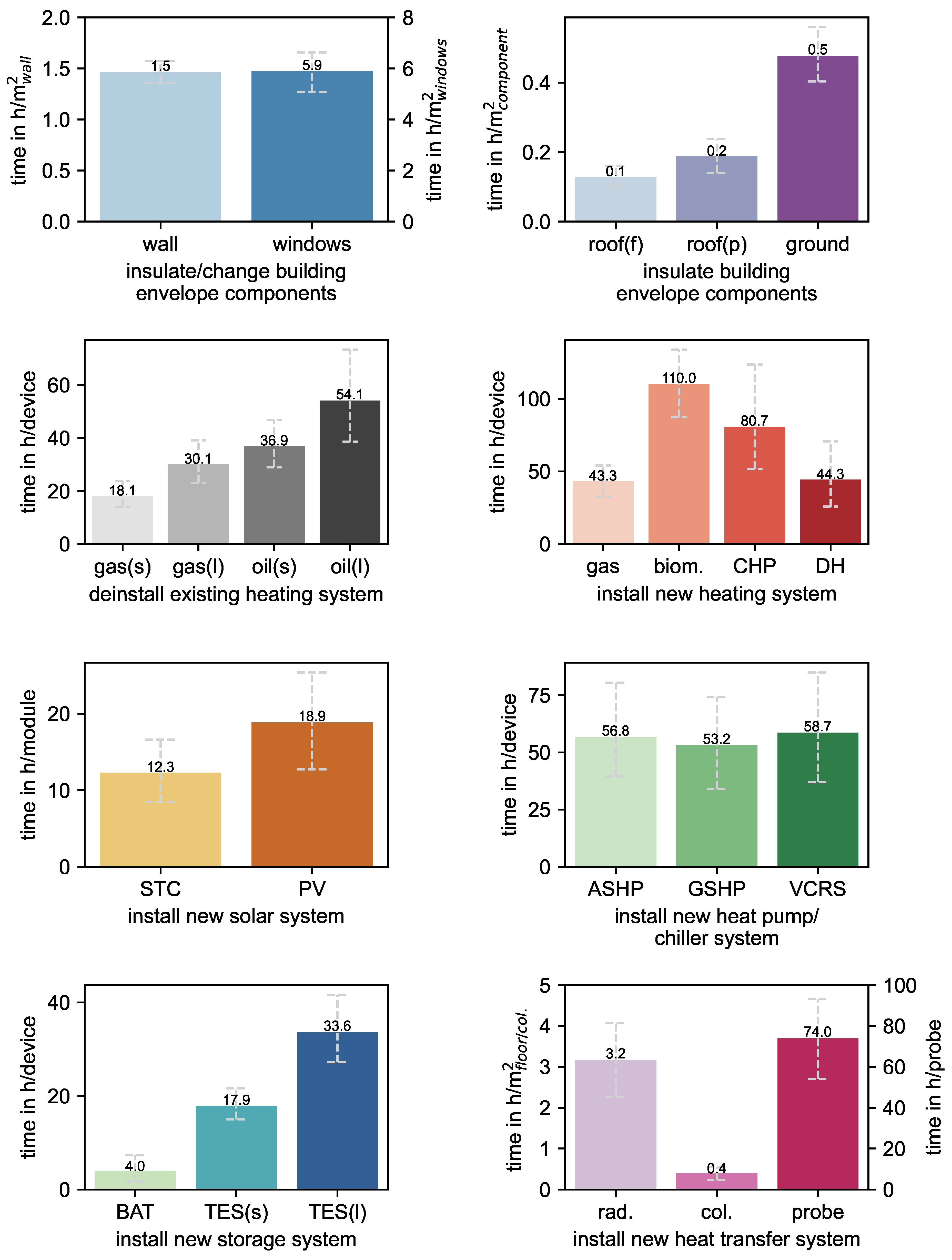
The aim of this research is to analyze the influence of limited craftwork capacities on a single building. Therefore, the capacity, i.e., the time that craftworkers need to realize a modernization measure, must be calculated. To handle craftswork capacities, we extended the model in this work by constraints (Equation (15)) to calculate the time craftworkers need to realize, i.e., to construct, a modernization measure in an existing building. This time $ct$ comprises a fixed part and an area- or power-specific part. The fixed part $c{t}^{\mathrm{fix}}$ represents aspects such as the modernization measure’s preparation and planning, journey to the building and delivery of tools and devices, and coordination with craftworkers of other fields and the building owner. The specific part $c{t}^{\mathrm{spec}}$ represents the actual implementation of the measure whose realization time is dependent on the area of a component (e.g., outer walls area to be insulated) or the size of a device (e.g., volume of a thermal energy storage).

$$\begin{array}{cc}\hfill & {\mathit{ct}}_{\mathit{dev},\mathit{i}}={\mathit{X}}_{\mathit{dev},\mathit{i}}·c{t}_{dev}^{\mathrm{fix}}+·{\mathit{p}}_{\mathit{dev},\mathit{i}}·c{t}_{dev}^{\mathrm{spec}}\forall dev,i\hfill \end{array}$$

(15a)

$$\begin{array}{cc}\hfill & {\mathit{ct}}_{\mathit{env},\mathit{i}}={\mathit{X}}_{\mathit{env},\mathit{i}}·c{t}_{env}^{\mathrm{fix}}+{\mathit{A}}_{\mathit{env},\mathit{i}}·c{t}_{env}^{\mathrm{spec}}\forall env\in \{groundfloor,outerwalls,roof,windows\},i\hfill \end{array}$$

(15b)

However, freely available data for this craftswork time ($c{t}^{\mathrm{fix}}$, $c{t}^{\mathrm{spec}}$) are missing. Therefore, 90 expert interviews with craftworkers of different fields were conducted by Richarz et al. [20]. Their method to collect the data and the generated data itself are described in the next subsection.

2.2. Data Generation for Modernization Measures’ Construction Time by Craftworkers

In the first step, an interview guideline was developed to ensure that every interview was conducted in the same way and quality regardless of who conducted it. Interviews were done with two methods: on the one hand via telephone and on the other hand via a questionnaire, based on the interview guideline, that was briefly explained and then filled out independently. Both procedures consisted of an information phase and a data phase.

In the information phase, the background of the research, and privacy of personal and company data were explained; permission was also requested to be allowed to use the data on craftwork realization times and to publish the data in an aggregated form. Furthermore, it was requested that average data for typical existing buildings and that the craftwork time should comprise the mentioned aspects of $c{t}^{\mathrm{fix}}$ and $c{t}^{\mathrm{spec}}$ in the former section. Finally, it was asked that waiting times for equipment, delays in deliveries or the construction process as well as additional time due to errors of other craftwork fields should not be considered.

In the data phase, the actual data were collected. This part was divided in the time for modernization measures concerning the building envelope, the uninstallation of existing devices and the installation of new devices. Average values as well as associated 95%-confidence intervals are shown in Figure 1.

Concerning envelope insulation and the change of windows, the experts could provide area-specific data and under the assumption that the whole area is insulated, no $c{t}^{\mathrm{fix}}$ is needed additionally. Confidence intervals are low for insulating outer walls and flat (f) roofs as well as changing windows, and slightly higher for insulating pitched (p) roofs. In general, the experts told that these values would be transferable to many different residential and non-residential buildings but added that values for complex building cubature or other special cases would vary.

Traditionally, European buildings are provided with heat by gas or oil boilers. One key message of the interviews was that the uninstallation of oil boilers is more time-consuming since the disposal is more complicated and an additional oil tank needs to be uninstalled. Since large (l) devices (>100 kW) must be disassembled into individual parts within the building and cannot be removed in one piece, their uninstallation needs more time than small (s) devices. The same effect applies to the installation of new thermal energy storages (TES).

Another interesting point was that the installation time of new heating devices in typical buildings is not dependent on their size but only per piece. Here, the data show higher average values and also higher confidence intervals for new technologies such as air- or ground-source heat pumps (ASHP, GSHP) compared to conventional suppliers such as gas boilers. Higher average values can be attributed to the fact that new technologies are more complex and higher confidence intervals to the different experiences that craftworkers have with these new devices.

For solar-powered systems, module-specific values could be provided and experts said that the surrounding infrastructure (e.g., cabling) increases linearly with the number of modules. Concerning heat transfer systems, we consider geothermal probes and collectors as well as the change of radiators that may be necessary to use low-temperature systems such as heat pumps. Installation times for probes were provided per piece where according to the experts, primarily the soil texture has a strong influence on the installation time and the depth of the probes is rather secondary. Values for collectors and radiator change could be provided per area.

According to the mentioned results, a fixed part $c{t}^{\mathrm{fix}}$ for installation times is only needed for TES and existing boilers. As shown in

Table 2. Disposition of the realization time by craftworkers into a fixed $c{t}^{\mathrm{fix}}$ and a specific part $c{t}^{\mathrm{spec}}$.

Device/Component	${\mathit{ct}}^{\mathbf{fix}}$	${\mathit{ct}}^{\mathbf{spec}}$
Installation of thermal energy storage (TES)	16.2 h	5.8 h/m${}^3$
Uninstallation of existing gas boiler	4.7 h	0.27 h/kW
Uninstallation of existing oil boiler	19.1 h	0.35 h/kW
All other modernization measures	0 h	Figure 1

, it was possible to dispose the generated data for these devices into a fixed and a specific part based on a linear regression.

2.3. Limited Resources

Figure 2 gives an overview of the developed method to handle limited resources in the used MIP.

In the first step (1), economical optimal modernization roadmaps are determined with the MIP without limiting resources. Second (2), out of the results of these roadmaps, we can quantify the needed energy resources $e^{\mathrm{econ}}$ and craftwork resources $c{t}^{\mathrm{econ}}$ in an economical optimal roadmap. Based on the following constraints for step three (3), we are able to limit these resources step by step in further optimization runs.

Basically, there are two options to limit resources $res$ in the model: Either, the sum of a resource over the whole roadmap may be limited by Equation (16) where $re{d}_{res}$ is the reduction parameter of a resource that can be set between 0 and 1. Thereby, roadmaps with different levels of a limited resource can be determined.

$$\begin{array}{cc}\hfill & \sum _{i=1}^n{\mathit{e}}_{\mathit{res},\mathit{i}}\le re{d}_{res}·e_{res}^{\mathrm{econ}}\forall res\in \{gas,pellet\}\hfill \end{array}$$

(16a)

$$\begin{array}{cc}\hfill & \sum _{i=1}^n(\sum _{dev}{\mathit{ct}}_{\mathit{dev},\mathit{i}}+\sum _{env}{\mathit{ct}}_{\mathit{env},\mathit{i}})\le re{d}_{res}·c{t}^{\mathrm{econ}}\hfill \end{array}$$

(16b)

The other possibility is to limit resources yearly via Equation (17).

$$\begin{array}{cc}\hfill & {\mathit{e}}_{\mathit{res},\mathit{i}}\le re{d}_{res}·e_{res}^{\mathrm{econ}}\forall res\in \{gas,pellet\},i\hfill \end{array}$$

(17a)

$$\begin{array}{cc}\hfill & \sum _{dev}{\mathit{ct}}_{\mathit{dev},\mathit{i}}+\sum _{env}{\mathit{ct}}_{\mathit{env},\mathit{i}}\le re{d}_{res}·c{t}^{\mathrm{econ}}\forall i\hfill \end{array}$$

(17b)

With limitations over the whole roadmap, general effects such as limited craftwork capacities for the realization of the energy transition in a specific country can be analyzed. By setting yearly constraints, developments of resources can be set. An example would be to assume the availability of biomass for buildings’ heating to increase or decrease over time.

Finally, it is possible to compare roadmaps of different levels in the fourth step (4). Within this paper, we focus on applying this method to limited craftswork capacities by the use of the generated data from the conducted expert interviews.

3. Application on a Typical Residential Building

The use case for this work is a typical German single-family house according to [60]. It was built in building age class 1969–1978 with corresponding heat transmission coefficients (outer walls: 0.83 W/m²K, roof: 0.41 W/m²K, ground floor: 0.68 W/m²K, windows: 2.8 W/m²K) calculated based on the material data base of [58]. The building has a floor area of 173.3 m², a outer wall area of 177.6 m², a window area of 34.2 m², a pitched roof area of 183.1 m², a ground floor area of 74 m² and a heated volume of 518 m³. In the initial state, heat is provided by an existing condensing gas boiler and distributed by radiators. Based on Germany’s emission goal for the building sector in 2030 and a linear continuation for 2040, the maximum emissions in these two years in relation to the emissions in the initial state are set to 32% and 16% respectively. All roadmaps are calculated with five-year steps.

In Figure 3, modernization roadmaps with six levels of craftwork capacities are shown. Therefore, the possible craftwork capacities were limited based on the the roadmap without limitations (100% craftwork capacity). The values of the two objectives are presented in the top subplot, as are the decisions of the model concerning the energy supply system (middle subplot) and the insulation standard of the envelope (bottom subplot). Furthermore, the existing state of the building is presented (ex.).

The first thing to be noticed is that roadmaps of all craftwork capacity levels can reduce total costs and cumulative emissions of the building compared to the existing state. This means that modernizations are not only saving emissions but are also economically sensible under recent boundary conditions. Although fewer modernization measures are realized with lower capacity levels, the total costs over the considered observation period increase almost linearly with reducing the capacity level. This is due to the fact that economically less optimal modernization measures are realized. Noteworthy is that although the set emission goals are met in all capacity levels, cumulative emissions increase with reducing the capacity level. Limited craftwork capacities thus also indirectly lead to higher emissions.

Concerning the energy supply system, decisions of the model vary significantly between the roadmaps of different capacity levels. Under recent boundary conditions, air-source heat pumps (hp air) combined with direct electrical heating (eh) are chosen. The hp can cover the majority of the heat demand while eh supports on very cold days. Self-generated electricity from photovoltaic modules (pv) lowers the emissions of the heat supply. The temporal offset between electricity generation and heat demand can be compensated to a large extent by the thermal energy storage (tes).

As the craftwork capacity is reduced, the existing boiler is used for longer, because fewer or smaller new devices can be installed. This is one reason for higher emissions at lower capacity levels. Another reason is the decreasing size of the pv system with reducing the capacity level because fewer modules take less time to be installed. With a decreasing pv system size, also the size of the eh decreases because less emission-free electricity is available. Since renovation decisions of the envelope change in the lowest capacity level, eh needs to be enlarged here which leads to higher costs and exponentially increasing emissions. Furthermore, the tes also decreases with reducing the capacity level and is not built at all after a capacity level of 60%. Hereby, hp’s electricity consumption from the public grid increases which leads not only to higher emissions but also to higher loads for the electricity grid.

The model considers that hps are only used at supply temperatures below 55 ${}^{\circ }\mathrm{C}$ and that hps work more efficiently at lower supply temperatures. The supply temperatures can be lowered by replacing the existing radiators or/and by insulating the building envelope. This the reason why insulation measures are chosen in every capacity level to lower the demand and enable the hp. Between the 100%- and 20%-capacity level, outer wall and ground floor insulation are chosen. Since roof insulations take less time, this measure is chosen in the lowest capacity level instead of insulating outer walls. From the analysis of the envelope renovation decisions, we can also conclude that for the examined building, ground floor insulation has the highest efficiency in terms of energy added value at the realization time.

4. Discussion

With the 1R1C demand model, the demand calculation can be done inside the optimization procedure. Thereby, interdependencies between the capacity of the building fabric and the operation of the supply system are considered. One example of such an interdependency is that the building can be overheated to store heat inside the building fabric. However, more detailed demand calculation approaches, such as energy simulations (e.g., EnergyPlus, Modelica) exist. Because of extensively higher computational efforts, these simulations cannot be integrated into the optimization procedure. Therefore, Petkov et al. [15] and Richarz et al. [14] determine modernization roadmaps and use demand profiles from energy simulation programs that are calculated in advance of the optimization procedure. The disadvantage of these approaches is the lack of consideration of the interdependencies between the capacity of the building fabric and the operation of the supply system.

Another aspect is the uncertainty of boundary conditions such as energy prices. Since modernization roadmaps of up to 30 years are determined, the boundary conditions are based on scenarios and prognoses that are naturally subject to uncertainties. It is possible to quantify the influences of these uncertainties with sensitivity analyses as proposed in [61]. Furthermore, stochastic (e.g., [12]) or robust (e.g., [16]) optimization approaches can handle the uncertainties inside the optimization.

Regarding the limitation of craftwork capacities, capacities may be distributed differently across craftwork areas (e.g., envelope insulation, heat supply system). Since our approach limits the sum of all craftwork areas together, further insights could be gained by distinguishing between the limitation of these areas.

5. Conclusions and Future Work

This work builds up on an optimization model for the determination of modernization roadmaps. We extended this model by a two-fold method to handle limited resources. The focus lies on limited energy resources and craftwork capacities. Data concerning the modernization measures’ realization times required by craftworkers was used out of recent research data that are based on 90 expert interviews.

An analysis of the craftwork data showed that most of the realization times for modernization measures at energy supply devices are independent of the device size. Confidence intervals for conventional devices (e.g., gas boilers) are smaller than those of newer devices (e.g., heat pumps) which is due to different experiences of craftworkers with newer devices. Realization times of insulation measures are linearly dependent on the size of the component to be insulated. In general, the interviewed experts reported that the requested time data are transferable to many different residential and non-residential buildings except untypical special buildings.

Based on the results of the application on a typical single-family house, limited craftwork capacities lead to higher total costs for a building’s modernization as well as to higher emissions by the modernized building energy systems and higher loads for the public electricity grid. Modernization roadmaps with limited craftwork capacities tend to use existing fossil fuels longer. Furthermore, our results show which measures should be done even in the case of limited craftwork capacities and which measures are omitted first: First, smaller thermal energy storages are implemented. If capacities are limited more, smaller pv systems are installed. Heat pumps combined with electrical direct heating are used even in roadmaps with very limited craftwork capacities. To make this heat supply system possible, the envelope is insulated at least at two possible components.

Future works could deal with analysis where only single fields of craftwork (e.g., insulation, heat) are limited. Further limited resources such as insulation materials and devices of the energy supply system could also be analyzed. Since the confidence intervals show uncertainties in the realization times, uncertainty methods such as sensitivity analyses or robust optimization could be applied. Furthermore, the method could be applied to other building types as well as to multiple buildings being optimized together in the model with limited resources, to see which building types should be prioritized in the case of limited resources.

References

1. International Energy Agency and the United Nations Environment Programme. 2018 Global Status Report: Towards a Zero-Emission, Efficient and Resilient Buildings and Construction Sector; UN Environment Programm: Nairobi, Kenya, 2018; Available online: https://wedocs.unep.org/handle/20.500.11822/27140 (accessed on 23 February 2023).
2. Pezzutto, S.; Zambotti, S.; Croce, S.; Zambelli, P.; Garegnani, G.; Scaramuzzino, C.; Pascuas, R.P.; Zubaryeva, A.; Haas, F.; Exner, D.; et al. Hotmaps Project, D2.3 WP2 Report—Open Data Set for the EU28, 2018; EURAC, e-think, TUW, Fraunhofer ISI, 2018. Available online: https://gitlab.com/hotmaps/building-stock (accessed on 23 February 2023).
3. Ma, Z.; Cooper, P.; Daly, D.; Ledo, L. Existing Building Retrofits: Methodology and State-of-the-Art. Energy Build. 2012, 55, 889–902. [Google Scholar] [CrossRef]
4. Costa-Carrapiço, I.; Raslan, R.; González, J.N. A Systematic Review of Genetic Algorithm-Based Multi-Objective Optimisation for Building Retrofitting Strategies towards Energy Efficiency. Energy Build. 2020, 210, 109690. [Google Scholar] [CrossRef]
5. Fodstad, M.; del Granado, P.C.; Hellemo, L.; Knudsen, B.R.; Pisciella, P.; Silvast, A.; Bordin, C.; Schmidt, S.; Straus, J. Next frontiers in energy system modelling: A review on challenges and the state of the art. Renew. Sustain. Energy Rev. 2022, 160, 112246. [Google Scholar] [CrossRef]
6. Panagiotidou, M.; Aye, L.; Rismanchi, B. Optimisation of multi-residential building retrofit, cost-optimal and net-zero emission targets. Energy Build. 2021, 252, 111385. [Google Scholar] [CrossRef]
7. Iturriaga, E.; Aldasoro, U.; Terés-Zubiaga, J.; Campos-Celador, A. Optimal renovation of buildings towards the nearly Zero Energy Building standard. Energy 2018, 160, 1101–1114. [Google Scholar] [CrossRef]
8. Schütz, T.; Schiffer, L.; Harb, H.; Fuchs, M.; Müller, D. Optimal design of energy conversion units and envelopes for residential building retrofits using a comprehensive MILP model. Appl. Energy 2017, 185, 1–15. [Google Scholar] [CrossRef]
9. Mans, M.; Remmen, P.; Scholl, A.; Fuchs, M.; Müller, D. Using Evolutionary Algorithms to Design Energy Supply Systems for a Changing Building Stock. In Proceedings of the 15th IBPSA Conference, San Francisco, CA, USA, 7–9 August 2017; pp. 1159–1168. [Google Scholar] [CrossRef]
10. D’Agostino, D.; Parker, D.; Epifani, I.; Crawley, D.; Lawrie, L. How will future climate impact the design and performance of nearly zero energy buildings (NZEBs)? Energy 2022, 240, 122479. [Google Scholar] [CrossRef]
11. Pecenak, Z.; Stadler, M.; Fahy, K. Efficient multi-year economic energy planning in microgrids. Appl. Energy 2019, 255, 113771. [Google Scholar] [CrossRef]
12. Bohlayer, M.; Bürger, A.; Fleschutz, M.; Braun, M.; Zoettl, G. Multi-period investment pathways - modeling approaches to design distributed energy systems under uncertainty. Appl. Energy 2021, 285, 116368. [Google Scholar] [CrossRef]
13. Mavromatidis, G.; Petkov, I. MANGO: A novel optimization model for the longterm, multi-stage planning of decentralized multi-energy systems. Appl. Energy 2021, 288, 116585. [Google Scholar] [CrossRef]
14. Richarz, J.; Henn, S.; Osterhage, T.; Müller, D. Optimal scheduling of modernization measures for typical non-residential buildings. Energy 2022, 238, 121871. [Google Scholar] [CrossRef]
15. Petkov, I.; Mavromatidis, G.; Knoeri, C.; Allan, J.; Hoffmann, V.H. MANGOret: An Optimization Framework for the Long-Term Investment Planning of Building Multi-Energy System and Envelope Retrofits. Appl. Energy 2022, 314, 118901. [Google Scholar] [CrossRef]
16. Richarz, J.; Hu, Y.; Wirtz, M.; Osterhage, T.; Müller, D. Robust optimal identifcation and scheduling of modernization measures for typical buildings. In Proceedings of the 17th IBPSA Conference, Bruges, Belgium, 1–3 September 2021. [Google Scholar] [CrossRef]
17. Richarz, J.; Hering, D.; Müller, D. Robust optimal multi-year modernization roadmaps for typical existing buildings. In Proceedings of the ECOS 2022: The 35th International Conference on Efficiency, Cost, Optimization, Simulation and Environmental Impact of Energy Systems, Copenhagen, Denmark, 4–7 July 2022. [Google Scholar] [CrossRef]
18. Seefeldt, F.; Rau, D.; Hoch, M. Fachkräftebedarf für die Energiewende in Gebäuden (en: Skilled Workers Needed for the Energy Transition in Buildings); Prognos AG: Berlin, Germany, 2018; Available online: https://www.prognos.com/de/projekt/fachkraeftebedarf-fuer-die-energiewende-gebaeuden (accessed on 2 May 2023).
19. Kenkmann, T.; Braungardt, S. Das Handwerk als Umsetzer der Energiewende im Gebäudesektor (en: Craftworkers as Implementers of the Energy Transition in the Building Sector); Öko-Institut e.V.: Freiburg, Germany, 2018; Available online: https://www.oeko.de/fileadmin/oekodoc/Handwerker-als-Umsetzer-Policy-Paper.pdf (accessed on 2 March 2023).
20. Richarz, J.; Fuchs, N.; Zurke, J.; Imberg, J.; Datsko, T.; Hering, D.; Müller, D. Realization Times of Energetic Modernization Measures for Buildings Based on Interviews with Craftworkers; Institute for Energy Efficient Buildings and Indoor Climate, RWTH Aachen University: Aachen, Germany, 2023; Available online: https://github.com/RWTH-EBC/CrafTiMod (accessed on 17 May 2023).
21. Prognos AG; Boston Consulting Group; Institute of Energy Economics at the University of Cologne (EWI); Fraunhofer ISI; Potsdam Institute for Climate Impact Research (PIK). Vergleich der “Big 5” Klimaneutralitätsszenarien (en: Comparison of the "Big 5" Climate Neutrality Scenarios); 2022; Available online: https://www.prognos.com/de/projekt/vergleich-der-big-5-klimaneutralitaetsszenarien (accessed on 19 January 2023).
22. Federal Ministry for Economic Affairs and Climate Action (BMWK). Integrierter Nationaler Energie- und Klimaplan (en: Integrated National Energy and Climate Plan). 2020. Available online: https://www.bmwk.de/Redaktion/DE/Textsammlungen/Energie/necp.html (accessed on 19 January 2023).
23. Zatti, M.; Gabba, M.; Freschini, M.; Rossi, M.; Gambarotta, A.; Morini, M.; Martelli, E. K-MILP: A Novel Clustering Approach to Select Typical and Extreme Days for Multi-Energy Systems Design Optimization. Energy 2019, 181, 1051–1063. [Google Scholar] [CrossRef]
24. Association of German Engineers (VDI) department of Technical Building Services. Guideline 2067: Economic Efficiency of Building Installations—Fundamentals and Economic Calculation; Technical Report; VDI Society Construction and Building Technology: Düsseldorf, Germany, 2010. [Google Scholar]
25. IINAS GmbH (Ed.) Globales Emissions-Modell Integrierter Systeme (en: Global Emissions Model of Integrated Systems); Internationales Institut für Nachhaltigkeitsanalysen und -Strategien: Darmstadt, Germany, 2023; Available online: https://iinas.org/downloads/gemis-downloads/ (accessed on 26 January 2023).
26. Luderer, G.; Kost, C.; Sörgel, D. (Eds.) Deutschland auf dem Weg zur Klimaneutralität 2045—Szenarien und Pfade im Modellvergleich, (Ariadne-Report); Potsdam Institute for Climate Impact Research: Potsdam, Germany, 2021; Available online: https://publications.pik-potsdam.de/pubman/item/item_26056 (accessed on 19 January 2023).
27. Burchardt, J.; Franke, K.; Herhold, P.; Hohaus, M.; Humpert, H.; Päivärinta, J.; Richenhagen, E.; Ritter, D.; Schönberger, S.; Schröder, J.; et al. KLIMAPFADE 2.0—Ein Wirtschaftsprogramm für Klima und Zukunft; Boston Consulting Group (BCG), Bundesverband der Deutschen Industrie e. V. (BDI): Berlin, Germany, 2021; Available online: https://issuu.com/bdi-berlin/docs/211021_bdi_klimapfade_2.0_-_gesamtstudie_-_vorabve (accessed on 19 January 2023).
28. DENA (Ed.) dena-Leitstudie Aufbruch Klimaneutralität; Deutsche Energie-Agentur GmbH: Berlin, Germany, 2021; Available online: https://www.dena.de/newsroom/publikationsdetailansicht/pub/abschlussbericht-dena-leitstudie-aufbruch-klimaneutralitaet/ (accessed on 19 January 2023).
29. Prognos; Öko-Institut; Wuppertal-Institut. Klimaneutrales Deutschland 2045; Stiftung Klimaneutralität, Agora Energiewende, prognos, Öko-Institut, Wuppertal Institut: Berlin, Germany, 2021; Available online: https://www.agora-energiewende.de/veroeffentlichungen/klimaneutrales-deutschland-2045-vollversion/ (accessed on 19 January 2023).
30. Mellwig, P.; Lempik, J.; Blömer, S.; Pehnt, M. Langfristszenarien für die Transformation des Energiesystems in Deutschland—Modul Gebäude; Consentec GmbH, Fraunhofer ISI, ifeu, TU Berlin: Karlsruhe, Germany, 2021; Available online: https://www.langfristszenarien.de/enertile-explorer-de/dokumente/ (accessed on 19 January 2023).
31. Prognos AG, Vereinigung der Bayerischen Wirtschaft e. V. (vbw). Strompreisprognose (en: Electricity Price Forecast). 2022. Available online: https://www.vbw-bayern.de/vbw/Themen-und-Services/Energie-Klima/Energie/Neue-Strompreisprognose-bis-2040.jsp (accessed on 8 March 2023).
32. DEPI. Energiekrise Beeinflusst Pelletpreis (en: Energy Crisis Influences Pellet Price); Technical Report; Deutsches Pelletinstitut: Berlin, Germany, 2022; Available online: https://depi.de/p/Energiekrise-beeinflusst-Pelletpreis-dQuuhhEc5W1R3MBAYoJVq7 (accessed on 8 March 2023).
33. BDEW. BDEW-Strompreisanalyse (en: BDEW Electricity Price Analysis); Technical Report; Bundesverband der Energie- und Wasserwirtschaft e.V.: Berlin, Germany, 2023; Available online: https://www.bdew.de/service/daten-und-grafiken/bdew-strompreisanalyse/ (accessed on 8 March 2023).
34. NT. Marktwertübersicht (en: Overview of the Solar Market Value); Technical Report; Netztransparenz: Berlin, Germany; Dortmund, Germany; Bayreuth, Germany; Stuttgart, Germany, 2023; Available online: https://www.netztransparenz.de/EEG/Marktpraemie/Marktwerte (accessed on 9 March 2023).
35. DEPI. Pelletpreiseanalyse (en: Analysis of Pellet Prices); Technical Report; Deutsches Pelletinstitut: Berlin, Germany, 2023; Available online: https://www.depi.de/pelletpreis-wirtschaftlichkeit#rrrg (accessed on 9 March 2023).
36. BDEW. BDEW-Gaspreisanalyse (en: BDEW Gas Price Analysis); Technical Report; Bundesverband der Energie- und Wasserwirtschaft e.V.: Berlin, Germany, 2023; Available online: https://www.bdew.de/service/daten-und-grafiken/bdew-gaspreisanalyse/ (accessed on 10 March 2023).
37. BCG. Perspectives on Experience; Technical Report; Boston Consulting Group Inc.: Boston, MA, USA, 1968. [Google Scholar]
38. Louwen, A.; Junginger, M.; Krishnan, S.; Derks, M. Analysis of the European Energy System under the Aspects of Flexibility and Technological Progress; Technical Report; Utrecht University, REFLEX: Utrecht, The Netherlands, 2018; Available online: http://reflex-project.eu/wp-content/uploads/2019/04/REFLEX_Stakeholder_WS_03_Technological_Learning_A.Louwen.pdf (accessed on 20 December 2022).
39. Kaufmann, T. Strategiewerkzeuge aus der Praxis: Analyse und Beurteilung der Strategischen Ausgangslage (en: Strategy Tools from Practice: Analysis and Assessment of the Strategic Starting Position); Springer: Berlin/Heidelberg, Germany, 2021. [Google Scholar] [CrossRef]
40. OWID. Solar (Photovoltaic) Panel Prices vs. Cumulative Capacity. 2021. Available online: https://ourworldindata.org/grapher/solar-pv-prices-vs-cumulative-capacity (accessed on 20 December 2022).
41. Weiss, W.; Spörk-Dür, M. Solar Heat Worldwide; Technical Report; International Energy Agency (IEA): Gleisdorf, Austria, 2022; Available online: https://www.iea-shc.org/Data/Sites/1/publications/Solar-Heat-Worldwide-2021.pdf (accessed on 8 January 2023).
42. EHPA. Annual Sales of Air-to-Water Heat Pumps in Europe from 1994 to 2020 with Forecasts until 2030; Technical Report; European Heat Pump Association: Brüssel, Belgium, 2022; Available online: www.ehpa.ord/market-data (accessed on 9 January 2023).
43. BAFA. Absatz von Mini-Blockheizkraftwerken in Deutschland in den Jahren 2010–2020 (en: Sales of Mini CHP Units in Germany in the Years 2010–2020); Technical Report; Bundesamt für Wirtschaft und Ausfuhrkontrolle: Eschborn, Germany, 2021; Available online: https://www.bafa.de/SharedDocs/Downloads/DE/Energie/kwk_statistik_zulassungen_kwk_anlagen.pdf;jsessionid=21096AAD543636498BEC1DD64857F296.2_cid381?__blob=publicationFile&v=19 (accessed on 15 January 2023).
44. BDH; TGA. Wärmeerzeuger Marktentwicklung in Deutschland 2000–2021 (en: Heat Generators Market Development in Germany 2000–2021; Technical Report; Bundesverband der deutschen Heizungsindustrie, TGA-Fachplaner: Stuttgart, Germany, 2022; Available online: https://www.tga-fachplaner.de/service/waermeerzeuger-marktentwicklung-deutschland-2000-bis-2021 (accessed on 4 February 2023).
45. DGfE. Mapping and Analyses of the Current and Future (2020–2030) Heating/Cooling Fuel Deployment (Fossil/Renewables); Technical Report; Directorate-General for Energy, Eurpäische Kommission: Brüssel, Belgium, 2016; Available online: https://energy.ec.europa.eu/publications/mapping-and-analyses-current-and-future-2020-2030-heatingcooling-fuel-deployment-fossilrenewables-1_en (accessed on 5 February 2023).
46. Craver, H.; BloombergNEF. Energ Storage Rising. 2021. Available online: https://wognews.net/news/2021/8/energy-storage-rising (accessed on 5 February 2023).
47. Ebert, V.; Günther, R.; Kremer, Z.; Pajor, R.; Bauer, D.; Drück, H.; Sommer, K.; Jahnke, K. Fahrplan Solarwarme-Strategie und Massnahmen der Solarwarme-Branche fur ein beschleunigtes Marktwachstum bis 2030 (en: Roadmap Solar Heating Strategy and Solar Heating Industry Measures for Accelerated Market Growth by 2030; Technical Report; BSW (Bundesverband Solarwirtschaft e.V.): Berlin, Germany, 2012; Available online: https://www.solarwirtschaft.de/fileadmin/media/pdf/120854_bsw_studie_st.pdf (accessed on 15 February 2023).
48. Weiss, M.; Junginger, M.; Patel, M.K. Learning Energy Efficiency—Experience Curves for Household Appliances and Space Heating, Cooling, and Lighting Technologies; Utrecht University: Utrecht, The Netherlands, 2008; Available online: https://dspace.library.uu.nl/handle/1874/32937 (accessed on 15 February 2023).
49. FhG ISE. Current and Future Cost of Photovoltaics. Long-Term Scenarios for Market Development, System Prices and LCOE of Utility-Scale PV Systems; Technical Report; Fraunhofer ISE: Freiburg, Germany; Agora Energiewende: Berlin, Germany, 2015; Available online: https://www.ise.fraunhofer.de/content/dam/ise/de/documents/publications/studies/AgoraEnergiewende_Current_and_Future_Cost_of_PV_Feb2015_web.pdf (accessed on 16 February 2023).
50. IRENA. Future of Solar Photovoltaic-Deployment, Investment, Technology, Grid Integration and Socio-Economic Aspects; Technical Report; International Renewable Energy Agency: Abu Dhabi, United Arab Emirates, 2019; Available online: https://www.irena.org/-/media/Files/IRENA/Agency/Publication/2019/Nov/IRENA_Future_of_Solar_PV_2019.pdf (accessed on 16 February 2023).
51. IEA. Technology Roadmap—Solar Heating and Cooling; Technical Report; International Energy Agency: Paris, France, 2012; Available online: https://www.iea.org/reports/technology-roadmap-solar-heating-and-cooling (accessed on 20 December 2022).
52. Harper, G. Doing Cold Smarter; Technical Report; Birmingham Energy Institute: Birmingham, UK, 2015; Available online: https://www.birmingham.ac.uk/research/energy/policy/cold/policy-commission-launch.aspx (accessed on 20 December 2022).
53. Fux, S.F.; Ashouri, A.; Benz, M.J.; Guzzella, L. EKF Based Self-Adaptive Thermal Model for a Passive House. Energy Build. 2014, 68, 811–817. [Google Scholar] [CrossRef]
54. SIA. Guideline 2024—Room Utilisation Data for Energy and Building Services (SIA 2024); Technical Report; Swiss Association of Engineers and Architects (SIA): Zurich, Switzerland, 2015. [Google Scholar]
55. DIN. DIN EN ISO 13790; Energy Performance of Buildings—Calculation of Energy Use for Space Heating and Cooling. German Institute for Standardization e.V.: Berlin, Germany, 2008. [Google Scholar]
56. DIN. DIN EN ISO 13786; Thermal Performance of Building Components—Dynamic Thermal Characteristics—Calculation Methods. German Institute for Standardization e.V.: Berlin, Germany, 2018. [Google Scholar]
57. Gurobi Optimization, LLC. Gurobi Optimizer Reference Manual. 2023. Available online: https://www.gurobi.com (accessed on 1 January 2023).
58. Remmen, P.; Lauster, M.; Mans, M.; Fuchs, M.; Osterhage, T.; Müller, D. TEASER: An Open Tool for Urban Energy Modelling of Building Stocks. J. Build. Perform. Simul. 2018, 11, 84–98. [Google Scholar] [CrossRef]
59. DIN. DIN EN ISO 6946; Building Components and Building Elements—Thermal Resistance and Thermal Transmittance—Calculation Methods. German Institute for Standardization e.V.: Berlin, Germany, 2008. [Google Scholar]
60. The Institute for Housing and Environment—Institut Wohnen und Umwelt GmbH (IWU). Typology Approach for Building Stock Energy Assessment. 2017. Available online: https://webtool.building-typology.eu (accessed on 31 January 2023).
61. Mavromatidis, G.; Orehounig, K.; Carmeliet, J. Uncertainty and Global Sensitivity Analysis for the Optimal Design of Distributed Energy Systems. Appl. Energy 2018, 214, 219–238. [Google Scholar] [CrossRef]
62. Mailach, B.; Oschatz, B. BDEW-Heizkostenvergleich Altbau (en: BDEW Heating Cost Comparison Old Building); Bundesverband der Energie-und Wasserwirtschaft e.V.: Dresden, Germany, 2022; Available online: https://www.bdew.de/energie/der-bdew-heizkostenvergleich/ (accessed on 7 November 2022).
63. WEKA Media GmbH & Co. KG (Ed.) Sirados Baudaten (en: Sirado’s Construction Data); WEKA Media GmbH & Co. KG: Kissing, Germany, 2023; Available online: https://www.sirados.de/ (accessed on 1 February 2023).
64. Hinz, E. Kosten Energierelevanter Bau- und Anlagenteile bei der Energetischen Modernisierung von Altbauten (en: Costs of Energy-Relevant Building and Plant Components in the Energy Modernization of Old Buildings); Technical Report; Institut Wohnen und Umwelt GmbH: Darmstadt, Germany, 2015; Available online: https://www.iwu.de/fileadmin/publikationen/handlungslogiken/2015_IWU_Hinz_Kosten-energierelevanter-Bau-und-Anlagenteile-bei-der-energetischen-Modernisierung-von-Altbauten.pdf (accessed on 7 November 2022).
65. Koch, T.; Achenbach, S.; Müller, A. Anpassung der Kostenfunktionen Energierelevanter Bau- und Anlagenteile bei der Energetischen Modernisierung von Altbauten auf das Preisniveau 2020 (en: Adjustment of the Cost Functions of Energy-Relevant Building and Plant Components in the Energy Modernization of Old Buildings to the Price Level 2020); Technical Report; Institut Wohnen und Umwelt GmbH: Darmstadt, Germany, 2021; Available online: https://www.iwu.de/fileadmin/publikationen/werkstattbericht/2021_IWU_KochEtAl_Werkstattbericht-Anpassung-Kostenfunktionen-2020.pdf (accessed on 7 November 2022).
Figure 1. Average data and error bars of the generated data for the realization time of modernization measures by craftworkers based on 90 expert interviews. Abbreviations: flat (f), pitched (p), small (s), large (l), biomass (biom.), combined heat and power (CHP), district heating (DH), solar thermal module (STC), photovoltaic modul (PV), air-source heat pump (ASHP), ground-source heat pump (GSHP), vapour-compression refrigeration system (VCRS), battery (BAT), thermal energy storage (TES), geothermal probes (probes), geothermal collector (col.), radiator (rad.).
Energies 16 04822 g001
Figure 2. Methodological steps to handle limited resources in the MIP.
Energies 16 04822 g002
Figure 3. Modernization roadmaps of a typical single family house under constrained craftwork capacities. Abbreviations: existing (ex.), electrical heating (eh), air-source heat pump (hp air), photovoltaic (pv), thermal energy storage (tes).
Energies 16 04822 g003